Variable selection and estimation for semi-parametric multiple-index models

Abstract

In this paper, we propose a novel method to select significant variables and estimate the corresponding coefficients in multiple-index models with a group structure. All existing approaches for single-index models cannot be extended directly to handle this issue with several indices. This method integrates a popularly used shrinkage penalty such as LASSO with the group-wise minimum average variance estimation. It is capable of simultaneous dimension reduction and variable selection, while incorporating the group structure in predictors. Interestingly, the proposed estimator with the LASSO penalty then behaves like an estimator with an adaptive LASSO penalty. The estimator achieves consistency of variable selection without sacrificing the root-$n$ consistency of basis estimation. Simulation studies and a real-data example illustrate the effectiveness and efficiency of the new method.

FLA

, and

1 Introduction

Suppose that $Y\in\mathbb{R}$ is a univariate response and $\mathbf{X}=(X_{1},\ldots,X_{p})^{\top}\in\mathbb{R}^{p}$ is a vector of predictors. A general goal of regression analysis is to characterize the conditional distribution of $Y$ given $\mathbf{X}$, or the conditional mean $E(Y|\mathbf{X})$. The theory of sufficient dimension reduction (Li [17] and Cook and Weisberg [10]) provides a framework for reducing the dimension of $\mathbf{X}$ while preserving information on regression. Let $\mathcal{S}$ denote a subspace of $\mathbb{R}^{p}$, and let $\mathbf{P}_{\mathcal{S}}$ denote the orthogonal projection onto $\mathcal{S}$ with respect to the usual inner product. If $Y$ and $\mathbf{X}$ are independent conditioned on $\mathbf{P}_{\mathcal{S}}\mathbf{X}$, then we say that $\mathcal{S}$ is a dimension reduction subspace. The intersection of all such subspaces, if itself satisfies the conditional independence, is defined to be the central subspace (Cook [6] and Yin, Li and Cook [38]). When only the mean response $E(Y|\mathbf{X})$ is of interest, sufficient dimension reduction can be defined in a similar fashion. Specifically, a subspace $\mathcal{S}$ is said to be a mean dimension reduction subspace if $Y$ is independent of $E(Y|\mathbf{X})$ given $\mathbf{P}_{\mathcal{S}}\mathbf{X}$. If the intersection of all mean dimension reduction subspaces is also a mean dimension reduction subspace, it is called the central mean subspace (Cook and Li [8]). In either case, sufficient dimension reduction permits us to restrict attention to a number $d\leq p$ of new predictors, expressed as linear combinations of the original ones: $\bm{\beta}_{1}^{\top}\mathbf{X},\ldots,\bm{\beta}_{d}^{\top}\mathbf{X}$, where $\{\bm{\beta}_{1},\ldots,\bm{\beta}_{d}\}$ is a basis of $\mathcal{S}$.

In the last two decades or so, a series of papers have considered issues related to dimension reduction in regression. There have primarily been two categories of estimation methods in the literature: inverse regression methods (Li [17], Cook and Weisberg [10] and Cook and Ni [9]) and direct regression methods (Härdle and Stoker [14], Xia et al. [34] and Yin and Li [37]). Inverse regression methods, despite being computationally simple and widely used, require strong assumptions on predictors such as the linearity condition (Li [17]), and often fail to estimate the central subspace exhaustively (Cook [6]). In contrast, the minimum average variance estimation (MAVE) method of Xia et al. [34] has proven effective in dimension reduction and estimation of complicated semi-parametric models. The root-$n$ consistency is still achievable for the MAVE estimate. Compared with other direct regression methods, the calculation for MAVE is much easier, and many efficient algorithms are available. Although MAVE was originally proposed for dimension reduction for the conditional mean, the idea was recently generalized to target the central subspace (Wang and Xia [28] and Yin and Li [37]). In this article, we are concerned mainly with predictors in the conditional mean.

Dimension reduction is a fundamental statistical problem in both theory and practice. The aforementioned dimension reduction methods, however, suffer from the difficulty of interpreting the results, because the new extracted predictors usually involve all of the original ones. To handle this problem, model-free variable selection, in the framework of sufficient dimension reduction, has attracted considerable attention in recent years. For example, Li, Cook and Nachtsheim [18] introduced test-based procedures, Bondell and Li [1] incorporated inverse regression estimation with LASSO (Tibshirani [25]) to obtain shrinkage inverse regression estimation, and Chen, Zou and Cook [5] proposed a unified method called coordinate-independent sparse estimation. See also Zhu et al. [41] and Wang, Xu and Zhu [31]. All these methods, which are largely “parametric” in nature, are based on inverse regression methods and thus suffer the drawbacks of strong design assumptions and poor finite-sample performance (Wang, Xu and Zhu [30]).

Exploring the idea of combining MAVE and LASSO, Wang and Yin [29] proposed a sparse MAVE method and Zeng, He and Zhu [39] designed for single-index models a lasso-type approach called sim-lasso. Because the sparse MAVE penalizes the index vectors directly, it is not a principled method for variable selection and only provides a sparse estimate for a basis matrix of the central mean subspace column by column. The use of the $l_{1}$ penalty function in Zeng, He and Zhu [39] is novel in that it penalizes the index vector and the norm of the derivative of link function simultaneously. However, the theoretical properties of sim-lasso, such as its consistency and convergence rate, have not yet been studied due to the interaction between the bandwidth and the penalty parameter. Further, it is nontrivial, if not impossible, to extend sim-lasso to deal with multiple-index models. Several papers have addressed the problem of semi-parametric variable selection for single-index models, and developed large sample properties. See, for instance, Liang et al. [20], Peng and Huang [21] and Wang, Xu and Zhu [30]. However, condition (vi) in Liang et al. [20] may not hold true and their approach could not be extended to handle multiple-index models. The penalized MAVE method in Wang, Xu and Zhu [30] was motivated by the reasoning that predictor selection can be realized through selection of nonvanishing rows of a basis matrix of the central mean subspace. A bridge penalty function was employed to penalize the $l_{1}$ norms of the rows of a basis matrix. Although the penalized MAVE performs well for multiple-index models in the numerical studies, its theoretical properties are established only for the special case of single-index models. This is because, condition (C5) in Wang, Xu and Zhu [30], which is also assumed in Peng and Huang [21], is hard to check and possibly invalid except for single-index models. To the best of our knowledge, semi-parametric variable selection for multiple-index models has thus far not been well studied.

In many engineering and scientific situations, however, predictors are naturally grouped. For example, in biological applications assayed genes or proteins can be grouped by biological pathways. Although useful, existing dimension reduction methods are generic and treat all predictors in $\mathbf{X}$ indiscriminately. To take advantage of such group knowledge, Li, Li and Zhu [19] proposed a group-wise sufficient dimension reduction method, called group-wise MAVE, which preserves full regression information in the conditional mean of $Y$ given $\mathbf{X}$ while exploiting the group structure among predictors. Generally, it is believed that incorporating group information into dimension reduction can facilitate interpretation of results and improve estimation accuracy as the number of unknown parameters has been greatly reduced.

As a simple illustration, we use an example to show the necessity of group-wise dimension reduction and variable selection. Consider a response model $Y=\bm{\beta}_{1}^{\top}\mathbf{X}_{1}+\sin(0.2\uppi\bm{\beta}_{2}^{\top}\mathbf{X}_{2})+0.5\varepsilon$, where $\mathbf{X}_{1}\in\mathbb{R}^{10}$, $\mathbf{X}_{2}\in\mathbb{R}^{10}$, $\bm{\beta}_{1}=(1,-1,0,\ldots,0)^{\top}$, $\bm{\beta}_{2}=(1,1,0,\ldots,0)^{\top}$, and all predictors and $\varepsilon$ are independent standard normal variables. Write $\mathbf{X}=(\mathbf{X}_{1}^{\top},\mathbf{X}_{2}^{\top})^{\top}$. Then the central mean subspace for $E(Y|\mathbf{X})$ is spanned by $(\bm{\beta}_{1}^{\top},\mathbf{0}_{10}^{\top})^{\top}$ and $(\mathbf{0}_{10}^{\top},\bm{\beta}_{2}^{\top})^{\top}$, where $\mathbf{0}_{10}$ is a $10\times 1$ vector of zeros. We then should rule out zeros and identify $\bm{\beta}_{1}$ and $\bm{\beta}_{2}$ or their linear combinations. A single but representative simulated data set with 150 observations was obtained, and the MAVE direction estimates were

$$(-0.624,0.647,0.006,0.057,0.034,-0.010,-0.013,0.033,0.023,-0.022,$$

$$\quad{}-0.275,-0.316,-0.002,-0.062,-0.057,0.010,0.005,-0.034,-0.028,-0.017)^{\top}$$

and

$$(0.141,0.379,-0.394,0.005,0.030,-0.313,-0.313,0.146,0.201,-0.341,$$

$$\quad 0.106,-0.022,-0.286,0.111,0.096,-0.047,-0.303,-0.073,-0.203,-0.226)^{\top}.$$

MAVE treats all predictors in $\mathbf{X}$ indiscriminately. While the first direction estimate seems reasonable, the second one is very poor, and thus the overall estimation accuracy must be poor. Given the prior information that $\mathbf{X}_{1}$ and $\mathbf{X}_{2}$ are two predictor groups, we apply group-wise MAVE, and the resulting estimates of $\bm{\beta}_{1}$ and $\bm{\beta}_{2}$ are respectively, given by

$$(0.698,-0.715,-0.035,-0.031,-0.010,-0.003,-0.001,0.010,-0.010,0.015)^{\top}$$

and

$$(0.717,0.666,-0.035,0.155,0.002,0.032,-0.008,0.111,-0.024,-0.058)^{\top}.$$

A substantial gain in accuracy has been achieved by incorporating the predictor group information. Nevertheless, in each group all the predictors are included in the extracted linear combination, although some coefficients are small, obscuring the fact that only the first two predictors are contributing factors. It is obvious that group-wise MAVE cannot be the base for both dimension reduction and variable selection. Therefore, a selection operator also plays an important role, and we will see that a shrinkage penalty will be useful for us to use group-wise MAVE to exclude irrelevant predictors from the model.

Two main features of this paper are listed below.

1. [2.]

2. We consider the problem of semi-parametric variable selection for multiple-index regression models. Although multiple-index models are popular in the statistics and econometrics literature, little work has been done on variable selection. We propose a shrinkage MAVE estimator by introducing a shrinkage factor for each row of an estimated basis matrix of the central mean subspace. For multiple-index models the proposed estimator is proved to be consistent in variable selection while retaining the root-$n$ consistency. However, although the estimation problem can be reformulated as a LASSO problem in spirit, the LASSO problem under study has an asymptotically singular design matrix (Knight and Fu [16]). This is because the MAVE procedure is a combination of nonparametric function estimation and direction estimation. This makes the theoretical investigation more complicated. To deal with this issue for single-index models, condition (C5) is assumed in Wang, Xu and Zhu [30], otherwise, the large sample properties are difficult to derive. For multiple-index models, the standard approach of LASSO with nonsingular designs fails to show the large sample properties. Therefore, in this paper, the results of mixed-rates asymptotics (Radchenko [22]) are adopted to derive the asymptotic behavior even the design matrix is asymptotically singular. This is a new skill about proving the asymptotics of the LASSO estimation for semi-parametric models. The interaction between the bandwidth and the penalty parameter now is explicitly shown in Theorem 2.1.

3. We propose a general knowledge-based method that accounts for prior group information. As we have explained before, the group structure leads to a reduction in the total number of parameters. Consequently, our method, which is motivated by and derives from dimension reduction, doubly alleviates the “curse of dimensionality”. As a by product, such a structure also makes the computation more efficient.

The paper is organized as follows. In Section 2.1, we review the group-wise minimum average variance estimation. In Section 2.2, we combine group-wise MAVE with the LASSO penalty, as an example, to propose a shrinkage group-wise MAVE estimator. This method does not require any restrictive design assumptions, and is capable of simultaneous dimension reduction and variable selection. The asymptotic properties of the new estimator are established in Section 2.3. We also use a criterion, which has the same form as the Bayesian information criterion (BIC; Schwarz [23]), to select the optimal tuning parameter. Moreover, we establish the consistency of the resulting BIC-type selector. Numerical studies are presented in Section 3. As many shrinkage penalties can also be applied, we then include the simulation results with two other penalties as well. All technical proofs are relegated to the Appendix.

2 Methodology

We begin with some basic notations and terminology. For a positive integer $m$, $\mathbf{I}_{m}$ stands for the $m\times m$ identity matrix. For an $m_{1}\times m_{2}$ matrix $\mathbf{A}$, $\operatorname{span}(\mathbf{A})$ represents the column space of $\mathbf{A}$ and $\mathbf{P}_{\mathbf{A}}$ represents the orthogonal projection onto $\operatorname{span}(\mathbf{A})$. For a subspace $\mathcal{S}$ of $\mathbb{R}^{m}$, if $\mathbf{A}$ is a matrix of full column rank and $\operatorname{span}(\mathbf{A})=\mathcal{S}$, then we call $\mathbf{A}$ a basis matrix of $\mathcal{S}$. Moreover, $\mathbf{P}_{\mathcal{S}}$ represents the projection onto $\mathcal{S}$, that is, $\mathbf{P}_{\mathcal{S}}=\mathbf{P}_{\mathbf{A}}$, where $\mathbf{A}$ is any basis matrix of $\mathcal{S}$. For an $m$-dimensional vector $\mathbf{w}=(w_{1},\ldots,w_{m})^{\top}$, $\operatorname{diag}(\mathbf{w})$ denotes a diagonal matrix whose diagonal entries starting in the upper left corner are $w_{1},\ldots,w_{m}$. We use $\mathbf{A}_{1}\oplus\cdots\oplus{\mathbf{A}_{g}}$, or simply $\bigoplus_{l=1}^{g}\mathbf{A}_{l}$, to denote a block diagonal matrix with matrices $\mathbf{A}_{1},\ldots,\mathbf{A}_{g}$ on the diagonal.

2.1 A short review

In this subsection, we review group-wise dimension reduction for the regression mean function and the group-wise minimum average variance estimation. We refer the reader to Li, Li and Zhu [19] for more details.

Let $\mathcal{S}_{1},\ldots,\mathcal{S}_{g}$ be subspaces of $\mathbb{R}^{p}$ that form an orthogonal decomposition of $\mathbb{R}^{p}$, that is, $\mathbb{R}^{p}=\mathcal{S}_{1}\oplus\cdots\oplus\mathcal{S}_{g}$, where $\oplus$ denotes the direct sum operator. If there are subspaces $\mathcal{T}_{l}\subseteq\mathcal{S}_{l}$ for $l=1,\ldots,g$ such that $E(Y|\mathbf{X})=E(Y|\mathbf{P}_{\mathcal{T}_{1}},\ldots,\mathbf{P}_{\mathcal{T}_{g}})$, then we say that $\mathcal{T}_{1}\oplus\cdots\oplus\mathcal{T}_{g}$ is a group-wise mean dimension reduction subspace with respect to $\{\mathcal{S}_{1},\ldots,\mathcal{S}_{g}\}$. Under very mild conditions (Yin, Li and Cook [38]), the intersection of all group-wise mean dimension reduction subspaces, with respect to a given orthogonal decomposition $\{\mathcal{S}_{1},\ldots,\mathcal{S}_{g}\}$, exists uniquely. We call this subspace the group-wise central mean subspace and denote it as $\mathcal{S}_{E(Y|\mathbf{X})}(\mathcal{S}_{1},\ldots,\mathcal{S}_{g})$. By definition,

$$\mathcal{S}_{E(Y|\mathbf{X})}(\mathcal{S}_{1},\ldots,\mathcal{S}_{g})=\mathcal{T}_{1}^{*}\oplus\cdots\oplus\mathcal{T}_{g}^{*}$$

for some subspaces $\mathcal{T}_{1}^{*}\subseteq\mathcal{S}_{1},\ldots,\mathcal{T}_{g}^{*}\subseteq\mathcal{S}_{g}$. Let $p_{l},d_{l}$ and $d$ denote the dimensions of $\mathcal{S}_{l}$, $\mathcal{T}_{l}^{*}$ and $\mathcal{S}_{E(Y|\mathbf{X})}(\mathcal{S}_{1},\ldots,\mathcal{S}_{g})$, respectively. Then we have $p=p_{1}+\cdots+p_{g}$ and $d=d_{1}+\cdots+d_{g}$.

Let $\bm{\Gamma}_{l}\in\mathbb{R}^{p\times p_{l}}$ be a basis matrix of $\mathcal{S}_{l}$, and let $\mathbf{V}_{l}=\bm{\Gamma}_{l}^{\top}\mathbf{X}\in\mathbb{R}^{p_{l}}$. We note that components of $\mathbf{V}_{l}$ correspond to predictors in group $l$, and all the group information contained in $\bm{\Gamma}_{l}$’s is available as prior knowledge. By construction, there are matrices $\mathbf{B}_{l}^{*}\in\mathbb{R}^{p_{l}\times d_{l}}$ for $l=1,\ldots,g$ such that $\operatorname{span}(\bm{\Gamma}_{l}\mathbf{B}_{l}^{*})=\mathcal{T}_{l}^{*}$. Write $\mathbf{B}^{*}=\bigoplus_{l=1}^{g}\mathbf{B}_{l}^{*}$. We are interested in estimating $\mathbf{B}^{*}$ or its column space $\operatorname{span}(\mathbf{B}^{*})$.

Li, Li and Zhu [19] proposed the group-wise MAVE estimator such that the matrix $\mathbf{B}^{*}=\bigoplus_{l=1}^{g}\mathbf{B}_{l}^{*}$ is the minimizer of

$$E\bigl{\{}Y-E\bigl{(}Y|\mathbf{B}_{1}^{\top}\mathbf{V}_{1},\ldots,\mathbf{B}_{g}^{\top}\mathbf{V}_{g}\bigr{)}\bigr{\}}^{2}$$

with respect to ${\mathbf{B}}_{1}\in\mathbb{R}^{p_{1}\times d_{1}},\ldots,{\mathbf{B}}_{g}\in\mathbb{R}^{p_{g}\times d_{g}}$, subject to $\mathbf{B}_{l}^{\top}\mathbf{B}_{l}=\mathbf{I}_{d_{l}}$ for $l=1,\ldots,g$.

Let $\mathbf{V}=(\mathbf{V}_{1}^{\top},\ldots,\mathbf{V}_{g}^{\top})^{\top}\in\mathbb{R}^{p}$ and $\mathbf{B}=\bigoplus_{l=1}^{g}\mathbf{B}_{l}$. Then we have

$$E\bigl{\{}Y-E\bigl{(}Y|\mathbf{B}_{1}^{\top}\mathbf{V}_{1},\ldots,\mathbf{B}_{g}^{\top}\mathbf{V}_{g}\bigr{)}\bigr{\}}^{2}=E\bigl{\{}\sigma_{\mathbf{B}}^{2}\bigl{(}\mathbf{B}^{\top}\mathbf{V}\bigr{)}\bigr{\}},$$

where $\sigma_{\mathbf{B}}^{2}(\mathbf{B}^{\top}\mathbf{V})=E[\{Y-E(Y|\mathbf{B}_{1}^{\top}\mathbf{V}_{1},\ldots,\mathbf{B}_{g}^{\top}\mathbf{V}_{g})\}^{2}|\mathbf{B}_{1}^{\top}\mathbf{V}_{1},\ldots,\mathbf{B}_{g}^{\top}\mathbf{V}_{g}]$ is the conditional variance of $Y$ given $\mathbf{B}_{1}^{\top}\mathbf{V}_{1},\ldots,\mathbf{B}_{g}^{\top}\mathbf{V}_{g}$.

Suppose that $\{(y^{i},\mathbf{v}^{i}),i=1,\ldots,n\}$ is a random sample from $(Y,\mathbf{V})$. Extending the MAVE idea, we can use local linear smoothing to estimate $\sigma_{\mathbf{B}}^{2}(\mathbf{B}^{\top}\mathbf{V})$. Specifically, for any given $\mathbf{v}^{0}\in\mathbb{R}^{p}$, we have the following approximation

$$\sigma_{\mathbf{B}}^{2}\bigl{(}\mathbf{B}^{\top}\mathbf{v}^{0}\bigr{)} \approx \sum_{j=1}^{n}\bigl{\{}y^{j}-E\bigl{(}Y|\mathbf{B}^{\top}\mathbf{V}=\mathbf{B}^{\top}\mathbf{v}^{j}\bigr{)}\bigr{\}}^{2}w_{j}^{0}$$

$$\approx \sum_{j=1}^{n}\Biggl{\{}y^{j}-a^{0}-\sum_{l=1}^{g}\mathbf{b}_{l}^{0\top}\mathbf{B}_{l}^{\top}\bigl{(}\mathbf{v}_{l}^{j}-\mathbf{v}_{l}^{0}\bigr{)}\Biggr{\}}^{2}w_{j}^{0},$$

where $w_{j}^{0}$’s are kernel weights such that $\sum_{j=1}^{n}w_{j}^{0}=1$, and $a^{0}+\sum_{l=1}^{g}\mathbf{b}_{l}^{0\top}\mathbf{B}_{l}^{\top}(\mathbf{v}_{l}^{j}-\mathbf{v}_{l}^{0})$ is the local linear expansion of $E(Y|\mathbf{B}^{\top}\mathbf{V}=\mathbf{B}^{\top}\mathbf{v}^{j})$ at $\mathbf{v}^{0}$.

Consequently, we can recover the group-wise central mean subspace by minimizing the objective function

$$\sum_{i=1}^{n}\sum_{j=1}^{n}\Biggl{\{}y^{j}-{{a}^{i}}-\sum_{l=1}^{g}\mathbf{b}_{l}^{i\top}\mathbf{B}_{l}^{\top}\bigl{(}\mathbf{v}_{l}^{j}-\mathbf{v}_{l}^{i}\bigr{)}\Biggr{\}}^{2}w_{j}^{i}$$ (1)

with respect to ${a}^{i}\in\mathbb{R}$, $\mathbf{b}_{1}^{i}\in\mathbb{R}^{d_{1}},\ldots,\mathbf{b}_{g}^{i}\in\mathbb{R}^{d_{g}}$, $i=1,\ldots,n$, and $\mathbf{B}_{l}\in\mathbb{R}^{p_{l}\times d_{l}}$ with $\mathbf{B}_{l}^{\top}\mathbf{B}_{l}=\mathbf{I}_{d_{l}}$ for $l=1,\ldots,g$. To allow the estimation to be adaptive to the regression structure, we follow the idea of refined MAVE (Xia et al. [34] and Li, Li and Zhu [19]) and adopt the weights

$$w_{j}^{i}=\frac{K_{h}\{\mathbf{B}^{\top}(\mathbf{v}^{j}-\mathbf{v}^{i})\}}{\sum_{j=1}^{n}K_{h}\{\mathbf{B}^{\top}(\mathbf{v}^{j}-\mathbf{v}^{i})\}},$$

where $K_{h}(\cdot)$ is a $d$-dimensional kernel with bandwidth $h$, and $\mathbf{B}$ is taken to be the current or latest estimate.

The minimization problem in (1) can be solved by fixing $({a}^{i},\mathbf{b}_{1}^{i},\ldots,\mathbf{b}_{g}^{i})$, $i=1,\ldots,n$, and fixing $\{\mathbf{B}_{l}\}_{l=1}^{g}$ alternatively. Thus, the calculation can be decomposed into two optimization problems both of which have simple analytic solutions. The details of the group-wise MAVE algorithm can be found in Section 3.2 of Li, Li and Zhu [19]. Let $\tilde{\mathbf{B}}=\bigoplus_{l=1}^{g}\tilde{\mathbf{B}}_{l}$ denote the group-wise minimum average variance estimator.

2.2 Shrinkage group-wise minimum average variance estimation

The group-wise MAVE method captures the full regression information in $E(Y|\mathbf{X})$ while preserving the group structure in $\mathbf{X}$. Specifically, it can provide a consistent estimator of $\mathbf{B}^{*}\mathbf{D}^{0}$ for some $d\times d$ nonsingular matrix $\mathbf{D}^{0}=\bigoplus_{l=1}^{g}\mathbf{D}_{l}^{0}$, where $\mathbf{D}_{l}^{0}\in\mathbb{R}^{d_{l}\times d_{l}}$ for $l=1,\ldots,g$. However, the elements of $\tilde{\mathbf{B}}_{l}$’s are usually nonzero. Consequently, the extracted predictor vector $\tilde{\mathbf{B}}_{l}^{\top}\mathbf{V}_{l}$ corresponding to group $l$ consists of linear combinations of all the predictors in that group. When there are a large number of predictors, one would expect that only a subset of predictors are relevant to the response variable. Write $\mathbf{V}=(V_{1},\ldots,V_{p})^{\top}$. According to Proposition 1 of Cook [7], $V_{s}$ is irrelevant if and only if the $s$th row of $\mathbf{B}^{*}$ is a zero vector. Further, it is easy to see that for any $d\times d$ nonsingular matrix $\mathbf{D}$, when a row of $\mathbf{B}^{*}$ is zero, the corresponding row of $\mathbf{B}^{*}\mathbf{D}$ is also zero, and vice versa. These observations motivate us to employ the state-of-the-art methods for simultaneous shrinkage estimation and variable selection, such as LASSO, to design a sparse version of the group-wise MAVE procedure which shrinkages some rows of $\tilde{\mathbf{B}}$ to be exactly zero vectors.

Define

$$\tilde{w}_{j}^{i}=\frac{K_{h}\{\tilde{\mathbf{B}}^{\top}({\mathbf{v}^{j}}-{\mathbf{v}}^{i})\}}{\sum_{j=1}^{n}K_{h}\{\tilde{\mathbf{B}}^{\top}({\mathbf{v}}^{j}-{\mathbf{v}}^{i})\}},\qquad i,j=1,\ldots,n.$$

For each $i=1,\ldots,n$, let $({\tilde{a}^{i}},\tilde{\mathbf{b}}_{1}^{i},\ldots,\tilde{\mathbf{b}}_{g}^{i})$ be the minimizer of

$$\sum_{j=1}^{n}\Biggl{\{}y^{j}-{{a}^{i}}-\sum_{l=1}^{g}{\mathbf{b}}_{l}^{i\top}\tilde{\mathbf{B}}_{l}^{\top}\bigl{(}{\mathbf{v}}_{l}^{j}-{\mathbf{v}}_{l}^{i}\bigr{)}\Biggr{\}}^{2}\tilde{w}_{j}^{i}.$$ (2)

In the sequel, we shall use an updated version of the group-wise minimum average variance estimator, $\tilde{\tilde{\mathbf{B}}}=\bigoplus_{l=1}^{g}\tilde{\tilde{\mathbf{B}}}_{l}$, which is the minimizer of

$$\sum_{i=1}^{n}\sum_{j=1}^{n}\Biggl{\{}y^{j}-{\tilde{a}^{i}}-\sum_{l=1}^{g}\tilde{\mathbf{b}}_{l}^{i\top}\mathbf{B}_{l}^{\top}\bigl{(}\mathbf{v}_{l}^{j}-\mathbf{v}_{l}^{i}\bigr{)}\Biggr{\}}^{2}\tilde{w}_{j}^{i}.$$ (3)

Definition 2.1.

A shrinkage group-wise minimum average variance estimator is defined as

$$\hat{\mathbf{B}}=\bigoplus_{l=1}^{g}\operatorname{diag}(\hat{\bm{\alpha}}_{l})\tilde{\tilde{\mathbf{B}}}_{l},$$

where the shrinkage index vectors $\hat{\bm{\alpha}}_{l}=(\hat{\alpha}_{l1},\ldots,\hat{\alpha}_{lp_{l}})^{\top}\in\mathbb{R}^{p_{l}}$ for $l=1,\ldots,g$ are determined by minimizing

$$\sum_{i=1}^{n}\sum_{j=1}^{n}\Biggl{[}y^{j}-{\tilde{a}^{i}}-\sum_{l=1}^{g}\tilde{{\mathbf{b}}}_{l}^{i\top}\bigl{\{}\operatorname{diag}(\bm{\alpha}_{l})\tilde{\tilde{\mathbf{B}}}_{l}\bigr{\}}^{\top}\bigl{(}{\mathbf{v}}_{l}^{j}-{\mathbf{v}}_{l}^{i}\bigr{)}\Biggr{]}^{2}\tilde{w}_{j}^{i}$$ (4)

with respect to $\bm{\alpha}_{l}=({\alpha}_{l1},\ldots,{\alpha}_{lp_{l}})^{\top}\in\mathbb{R}^{p_{l}}$, $l=1,\ldots,g$, subject to $\sum_{l=1}^{g}\sum_{s=1}^{p_{l}}|\alpha_{ls}|\leq\tau_{n}$ for some $\tau_{n}\geq 0$.

To solve the above optimization problem, we note that (4) can be re-expressed as

$$\sum_{i=1}^{n}\sum_{j=1}^{n}\Biggl{\{}y^{j}-{\tilde{a}^{i}}-\sum_{l=1}^{g}{\tilde{\mathbf{b}}}_{l}^{i\top}\tilde{\tilde{\mathbf{B}}}_{l}{\vphantom{\tilde{B}}\!\!}^{\top}\operatorname{diag}\bigl{(}\mathbf{v}_{l}^{j}-\mathbf{v}_{l}^{i}\bigr{)}\bm{\alpha}_{l}\Biggr{\}}^{2}\tilde{w}_{j}^{i}.$$

Equivalently, the shrinkage index vectors minimize

$$\sum_{i=1}^{n}\sum_{j=1}^{n}\Biggl{\{}y^{j}-{\tilde{a}^{i}}-\sum_{l=1}^{g}{\tilde{\mathbf{b}}}_{l}^{i\top}\tilde{\tilde{\mathbf{B}}}_{l}{\vphantom{\tilde{B}}\!\!}^{\top}\operatorname{diag}\bigl{(}\mathbf{v}_{l}^{j}-\mathbf{v}_{l}^{i}\bigr{)}\bm{\alpha}_{l}\Biggr{\}}^{2}\tilde{w}_{j}^{i}+\lambda_{n}\sum_{l=1}^{g}\sum_{s=1}^{p_{l}}|\alpha_{ls}|$$ (5)

for some tuning parameter $\lambda_{n}\geq 0$. As a result, commonly-used LASSO algorithms, such as those of Efron et al. [11] and Friedman, Hastie and Tibshirani [13], can be applied to obtain the shrinkage index vectors $\hat{\bm{\alpha}}_{l}$ for $l=1,\ldots,g$.

When $\tau_{n}\geq p$, the indices $\hat{\alpha}_{ls}=1$ for all $l=1,\ldots,g$ and $s=1,\ldots,p_{l}$, and so $\hat{\mathbf{B}}$ reduces to the usual group-wise MAVE estimator $\tilde{\tilde{\mathbf{B}}}$. As $\tau_{n}$ gradually decreases, some of the indices are shrunk to zero, which means some rows of $\hat{\mathbf{B}}$ are zero; that is, the corresponding predictors are irrelevant to the response variable given the other predictors.

2.3 Asymptotic theory

We next study the large-sample properties of the proposed method. For an $m_{1}\times m_{2}$ matrix $\mathbf{A}$, we say that $\mathbf{A}$ is row-sparse if some of its rows are zero. Let $\mathcal{I}(\mathbf{A})\subseteq\{1,\ldots,m\}$ denote the subset of indices corresponding to nonzero rows of $\mathbf{A}$. Clearly, the notion of row-sparseness is nonsingular-transformation independent, since for any $m_{2}\times m_{2}$ nonsingular matrix $\mathbf{O}$, $\mathcal{I}(\mathbf{A})=\mathcal{I}(\mathbf{A}\mathbf{O})$. Suppose that $\mathbf{B}^{*}=\bigoplus_{l=1}^{g}\mathbf{B}_{l}^{*}$ is row-sparse. Without loss of generality, we assume that for $l=1,\ldots,g$ the first $q_{l}$ rows of $\mathbf{B}_{l}^{*}$ are nonzero, that is, $\mathcal{I}(\mathbf{B}_{l}^{*})=\{1,\ldots,q_{l}\}$. The following theorem concerns the asymptotic behavior of shrinkage group-wise MAVE.

Theorem 2.1.

Suppose that the regularity conditions (A1)–(A6) given in the Appendix hold. If $\lambda_{n}\rightarrow\infty$ and $\lambda_{n}n^{-1/2}h^{-2}\rightarrow 0$, then we have (

• 2)]

• selection consistency: $P\{\mathcal{I}(\hat{\mathbf{B}}_{l})=\mathcal{I}(\mathbf{B}_{l}^{*}),l=1,\ldots,g\}\rightarrow 1$, and

• root-$n$ consistency: $\hat{\mathbf{B}}_{l}=\mathbf{B}_{l}^{*}\mathbf{D}_{l}^{0}+\mathrm{O}_{P}(n^{-1/2})$ for $l=1,\ldots,g$.

Theorem 2.1, part (1), demonstrates that the shrinkage group-wise MAVE method can efficiently remove unimportant predictors, while part (2) implies that the estimator that corresponds to relevant predictors is root-$n$ consistent. As we can see, the result is very similar to that of adaptive LASSO for linear models (Zou [42]). In fact, we shall show in the proof that shrinkage group-wise MAVE is closely related to an adaptive LASSO problem. A similar phenomena can be found in Bondell and Li [1] where they studied the shrinkage inverse regression estimation. However, unlike linear models, we need to study the interplay between the bandwidth $h$ and the penalty parameter $\lambda$. This is explicitly shown in Theorem 2.1 in which we require that $\lambda\rightarrow\infty$ and $\lambda n^{-1/2}h^{-2}\rightarrow 0$. We also note that, although it is possible to derive the asymptotic distribution, the form of the asymptotic variance is rather complicated and thus is not pursued here.

As a direct application we consider the special case when $g=1$, that is, there is no group information available. It follows that the shrinkage MAVE estimator possesses exactly the same properties.

Corollary 2.1.

Assume that $g=1$, and that the regularity conditions (A1)–(A6) given in the Appendix hold. If $\lambda_{n}\rightarrow\infty$ and $\lambda_{n}n^{-1/2}h^{-2}\rightarrow 0$, then we have (

• 2)]

• selection consistency: $P\{\mathcal{I}(\hat{\mathbf{B}})=\mathcal{I}(\mathbf{B}^{*})\}\rightarrow 1$, and

• root-$n$ consistency: $\hat{\mathbf{B}}=\mathbf{B}^{*}\mathbf{D}^{0}+\mathrm{O}_{P}(n^{-1/2})$.

The attractive properties of shrinkage group-wise MAVE depend critically on an appropriate choice of the tuning parameter, for which prediction based criteria such as generalized cross-validation have been commonly used in practice. However, it is well known that this practice tends to produce over-fitted models. For model selection consistency, it has been verified that tuning parameter selectors with the Bayesian information criterion are able to identify the true model consistently; see for example Wang, Li and Tsai [27] and Wang and Leng [26]. In the following, we propose a criterion which is similar in form to the classical Bayesian information criterion.

Let $\hat{\bm{\alpha}}(\lambda)=(\hat{\bm{\alpha}}_{1}^{\top},\ldots,\hat{\bm{\alpha}}_{g}^{\top})^{\top}$. Write $\hat{\bm{\alpha}}(\lambda)=(\hat{\alpha}_{1},\ldots,\hat{\alpha}_{p})^{\top}$ and $\mathbf{V}=(V_{1},\ldots,V_{p})^{\top}$. We use the notation $\mathcal{M}=\{r_{1},r_{2},\ldots,r_{p^{*}}\}\subseteq\{1,\ldots,p\}$ to denote an arbitrary candidate model which includes predictors $\{V_{s},s\in\mathcal{M}\}$. Let $k_{1}=0$ and $k_{l}=p_{1}+\cdots+p_{l-1}$ for $l=2,\ldots,g$. Then, $\mathcal{M}_{F}=\{1,\ldots,p\}$ and $\mathcal{M}_{T}=\bigcup_{l=1}^{g}\{k_{l}+1,\ldots,k_{l}+q_{l}\}$ represent the full model and the true model, respectively. Finally, we use $|\mathcal{M}|$ to denote the size of the model $\mathcal{M}$.

Let $\mathcal{M}_{\lambda}=\{s:\hat{\alpha}_{s}\neq 0\}$ be the model that is identified by $\hat{\bm{\alpha}}(\lambda)$ or $\hat{\mathbf{B}}$. Define

$$\operatorname{RSS}_{\lambda}=\sum_{i=1}^{n}\sum_{j=1}^{n}\Biggl{\{}y^{j}-{\tilde{a}^{i}}-\sum_{l=1}^{g}{\tilde{\mathbf{b}}}_{l}^{i\top}\tilde{\tilde{\mathbf{B}}}_{l}{\vphantom{\tilde{B}}\!\!}^{\top}\operatorname{diag}\bigl{(}\mathbf{v}_{l}^{j}-\mathbf{v}_{l}^{i}\bigr{)}\hat{\bm{\alpha}}_{l}\Biggr{\}}^{2}\tilde{w}_{j}^{i}.$$

We select the optimal $\lambda$ by minimizing

$$\operatorname{BIC}_{\lambda}=\log(\operatorname{RSS}_{\lambda})+\operatorname{df}_{\lambda}\frac{\log(n)}{n},$$ (6)

where $\operatorname{df}_{\lambda}$ denotes the effective number of parameters in the shrinkage group-wise MAVE estimator. The resulting optimal regularization parameter is denoted by $\hat{\lambda}_{\mathrm{BIC}}$. Following the discussion of Zou, Hastie and Tibshirani [43] about the degrees of freedom of the LASSO estimator, we approximate $\operatorname{df}_{\lambda}$ by $d_{1}|\mathcal{M}_{\lambda}^{1}|+\cdots+d_{g}|\mathcal{M}_{\lambda}^{g}|$, where $\mathcal{M}_{\lambda}^{l}$ represents the index set of identified predictors in group $l$.

We now establish the asymptotic property of the BIC-type tuning parameter selector.

Theorem 2.2.

Suppose that the regularity conditions (A1)–(A6) given in the Appendix hold. Then we have $P(\mathcal{M}_{\hat{\lambda}_{\mathrm{BIC}}}=\mathcal{M}_{T})\rightarrow 1$.

1. [3.]

2. Mixed-rates behavior naturally arises in the estimation of semi-parametric models. As shown in the proof of Theorem 2.1, the objective function (5) can be decomposed into two components with different convergent rates. As a result, the standard approach does not yield the complete limiting behavior of the estimator. Fortunately, we are able to derive the asymptotic behavior by directly applying results from mixed-rates asymptotics (Radchenko [22]).

3. In practice, one may use a concave penalty other than the LASSO penalty. We have tried using the smoothly clipped absolute deviation penalty (Fan and Li [12]) and the minimax concave penalty (Zhang [40]), and have found that the resulting estimators enjoy the same properties. See Section 3 for a numerical comparison of these methods. Consider again the illustrative example in Section 1, the proposed sparse group-wise MAVE method, when the smoothly clipped absolute deviation penalty is used, yielded the direction estimates

   $$(0.702,-0.712,0,\ldots,0)^{\top}\quad\mbox{and}\quad(0.722,0.692,0,0.027,0,\ldots,0)^{\top}.$$

   As we can see, all except one of the coordinates corresponding to irrelevant predictors were correctly shrunk to zero.

4. The result here is applicable to a general class of semi-parametric models. In particular, it provides an alternative method for estimation and selection for partially linear single-index models in which two groups exist naturally (Xia and Härdle [33]). Further, the new method can be adjusted to handle dimension reduction and variable selection with censored data (Xia, Zhang and Xu [35]).

5. Although in this paper we focus on shrinkage estimation of the group-wise central mean subspace, the same strategy can be used to target the group-wise central subspace. To see this, we note that Wang and Xia [28] have modified MAVE to estimate the central subspace, and so group-wise MAVE can be modified in a similar way to estimate the group-wise central subspace; see Section 8 of Li, Li and Zhu [19] for more discussion. To conclude, we believe that these efforts would enhance the usefulness of the shrinkage MAVE method in data analysis.

3 Numerical studies

3.1 Simulation studies

In this subsection, we use simulations to evaluate the finite-sample performance of the shrinkage group-wise MAVE method. For comparison we consider the LASSO penalty, the smoothly clipped absolute deviation (SCAD) penalty and the minimax concave penalty (MCP) in the simulation. The resulting estimators, including group-wise MAVE, are denoted by SgMAVE-LASSO, SgMAVE-SCAD, SgMAVE-MCP and gMAVE, respectively. Throughout the following numerical studies we adopt the Gaussian kernel and use the optimal bandwidth $h=\{4/(d+2)\}^{1/(d+4)}n^{-1/(d+4)}$. The R code that we used for group-wise MAVE is available at http://www4.stat.ncsu.edu/~li/software.html. SgMAVE-LASSO is computed using the least angle regression algorithm (Efron et al. [11]), while SgMAVE-SCAD and SgMAVE-MCP are computed using the coordinate descent algorithms described by Breheny and Huang [2]. The entire R code can be requested from the authors.

To evaluate estimation accuracy, we compute the vector correlation coefficient (VCC), which is defined as $(\prod_{t=1}^{d_{l}}\phi_{t}^{2})^{1/2}$, and the trace correlation coefficient (TCC), which is defined as $({d_{l}}^{-1}\sum_{t=1}^{d_{l}}\phi_{t}^{2})^{1/2}$, where the $\phi_{t}^{2}$’s are the eigenvalues of the matrix $\hat{\mathbf{B}}_{l}^{\top}\mathbf{B}_{l}^{*}\mathbf{B}_{l}^{*\top}\hat{\mathbf{B}}_{l}$. These two measures range between 0 and 1, with larger values indicating a more accurate estimator; see Ye and Weiss [36] for more information. We also employ three summary statistics to assess how well the methods select predictors: the average model size (MS), which is the average number of nonzero rows of $\hat{\mathbf{B}}_{l}$; the true positive rate (TPR), which is the average fraction of nonzero rows of $\hat{\mathbf{B}}_{l}$ associated with relevant predictors; and the false positive rate (FPR), which is the average fraction of nonzero rows of $\hat{\mathbf{B}}_{l}$ associated with irrelevant predictors. Both TPR and FPR range between 0 and 1, and ideally, we wish to have TPR to be close to 1 and FPR to be close to 0 at the same time. We report the results using the BIC-type criterion (6) to select tuning parameters.

The predictor vector $\mathbf{V}=(\mathbf{V}_{1}^{\top},\ldots,\mathbf{V}_{g}^{\top})^{\top}$ is generated from $N(\mathbf{0}_{p},\bm{\Sigma})$ in each example. We examine two commonly-used correlation structures among the predictors. The first is autoregressive, $\Sigma_{st}=0.5^{|s-t|}$ for all $s,t=1,\ldots,p$. Consequently, the predictors with large distances in order are expected to be mutually independent approximately. The second is compound symmetry, $\Sigma_{ss}=1$ and $\Sigma_{st}=0.5$ for any $s\neq t$, so all the predictors are equally correlated with each other.

Example 3.0.

In this experiment, we set

$$(g,p_{1},p_{2},d_{1},d_{2},q_{1},q_{2})=(2,20,20,1,1,3,2).$$

Thus, there are two groups, $\mathbf{V}_{1}$ and $\mathbf{V}_{2}$, and each group consists of twenty predictors. Further, each predictor group is connected with the response variable through a single linear combination. Specifically, the response variable is generated from each of the following three models:

$$Y = \bm{\beta}_{1}^{\top}\mathbf{V}_{1}\bigl{(}1+\bm{\beta}_{2}^{\top}\mathbf{V}_{2}\bigr{)}+0.5\varepsilon,$$ (7)

$$Y = \bm{\beta}_{1}^{\top}\mathbf{V}_{1}/\bigl{\{}0.5+\bigl{(}1.5+\bm{\beta}_{2}^{\top}\mathbf{V}_{2}\bigr{)}^{2}\bigr{\}}+0.5\varepsilon,$$ (8)

$$Y = \exp\bigl{(}0.5\bm{\beta}_{1}^{\top}\mathbf{V}_{1}\bigr{)}+\sin\bigl{(}0.2\uppi\bm{\beta}_{2}^{\top}\mathbf{V}_{2}\bigr{)}+0.5\varepsilon,$$ (9)

where $\bm{\beta}_{1}=(1,1,1,0,\ldots,0)^{\top}$, $\bm{\beta}_{2}=(1,1,0,\ldots,0)^{\top}$, $\varepsilon\thicksim N(0,1)$, and $\varepsilon$ is independent of all predictors. We let $n=200$.

Table 3.1 presents the simulation results based on 200 data replications for these three models. As we can see, all methods considered show very good performance, but the shrinkage ones often achieve higher estimation accuracy than the one without shrinkage. Further, although none of the three shrinkage methods can universally dominate the other two competitors, SgMAVE-SCAD and SgMAVE-MCP tend to produce sparser solutions than SgMAVE-LASSO. Finally, the performance of the group-wise MAVE estimator and its shrinkage versions is only slightly affected by the correlation structure among the predictors.

==0pt Summary of Example 1. The average vector correlation coefficient (VCC) with standard error in parentheses, the average number of predictors selected (MS), true positive rate (TPR) and false positive rate (FPR), based on 200 data replications, are reported $\bm{\beta}_{1}$ $\bm{\beta}_{2}$ VCC MS TPR FPR VCC MS TPR FPR Model (7): autoregressive correlation gMAVE 0.9963 (0.0239) 0.9905 (0.0780) SgMAVE-LASSO 0.9895 (0.0996) 4.1550 0.9900 0.1692 0.9896 (0.0997) 3.1850 0.9900 0.1506 SgMAVE-SCAD 0.9976 (0.0207) 3.0450 1.0000 0.0064 0.9898 (0.0997) 2.0150 0.9900 0.0043 SgMAVE-MCP 0.9977 (0.0193) 3.1200 1.0000 0.0171 0.9897 (0.0997) 2.0550 0.9900 0.0093 Model (7): compound symmetry gMAVE 0.9923 (0.0704) 0.9818 (0.1108) SgMAVE-LASSO 0.9933 (0.0709) 4.8450 0.9950 0.2657 0.9808 (0.1254) 4.0300 0.9900 0.2562 SgMAVE-SCAD 0.9935 (0.0710) 3.1400 0.9950 0.0221 0.9811 (0.1252) 2.1300 0.9875 0.0193 SgMAVE-MCP 0.9934 (0.0710) 3.1950 0.9950 0.0300 0.9805 (0.1294) 2.1050 0.9825 0.0175 Model (8): autoregressive correlation gMAVE 0.9771 (0.0137) 0.9735 (0.0538) SgMAVE-LASSO 0.9885 (0.0104) 5.5350 1.0000 0.3621 0.9846 (0.0477) 4.1400 0.9975 0.2681 SgMAVE-SCAD 0.9915 (0.0103) 3.7300 1.0000 0.1042 0.9849 (0.0557) 2.5700 0.9950 0.0725 SgMAVE-MCP 0.9886 (0.0116) 4.0100 1.0000 0.1442 0.9837 (0.0550) 2.5750 0.9950 0.0731 Model (8): compound symmetry gMAVE 0.9739 (0.0177) 0.9432 (0.1535) SgMAVE-LASSO 0.9856 (0.0120) 5.7650 1.0000 0.3950 0.9450 (0.1940) 3.7450 0.9625 0.2275 SgMAVE-SCAD 0.9896 (0.0130) 3.8300 1.0000 0.1185 0.9486 (0.1923) 2.3500 0.9600 0.0537 SgMAVE-MCP 0.9858 (0.0132) 4.0500 1.0000 0.1500 0.9438 (0.2031) 2.3000 0.9550 0.0487

==0pt (Continued) $\bm{\beta}_{1}$ $\bm{\beta}_{2}$ VCC MS TPR FPR VCC MS TPR FPR Model (9): autoregressive correlation gMAVE 0.9955 (0.0026) 0.9648 (0.0214) SgMAVE-LASSO 0.9981 (0.0019) 5.2600 1.0000 0.3228 0.9879 (0.0158) 3.6250 1.0000 0.2031 SgMAVE-SCAD 0.9984 (0.0019) 3.8250 1.0000 0.1178 0.9832 (0.0726) 2.6850 0.9950 0.0868 SgMAVE-MCP 0.9981 (0.0020) 3.6450 1.0000 0.0921 0.9874 (0.0191) 2.5650 1.0000 0.0706 Model (9): compound symmetry gMAVE 0.9954 (0.0023) 0.9546 (0.0401) SgMAVE-LASSO 0.9974 (0.0019) 5.8050 1.0000 0.4007 0.9766 (0.0384) 3.9250 1.0000 0.2406 SgMAVE-SCAD 0.9981 (0.0019) 4.0600 1.0000 0.1514 0.9792 (0.0517) 2.8800 0.9975 0.1106 SgMAVE-MCP 0.9977 (0.0021) 3.7850 1.0000 0.1121 0.9786 (0.0499) 2.5950 0.9975 0.0750

Example 3.0.

In this experiment, we set

$$(g,p_{1},p_{2},d_{1},d_{2},q_{1},q_{2})=(2,20,20,2,1,q_{1},2).$$

Thus, there are two groups, $\mathbf{V}_{1}$ and $\mathbf{V}_{2}$, and each group consists of twenty predictors. Further, the first predictor group is connected with the response variable through two linear combinations and the second predictor group is connected with the response variable through a single linear combination. The regression model is

$$Y=2.5\bm{\beta}_{11}^{\top}\mathbf{V}_{1}/\bigl{\{}0.5+\bigl{(}1.5+\bm{\beta}_{12}^{\top}\mathbf{V}_{1}\bigr{)}^{2}\bigr{\}}+\bm{\beta}_{2}^{\top}\mathbf{V}_{2}+0.5\varepsilon,$$ (10)

where $\bm{\beta}_{11}=(1,1,0,\ldots,0)^{\top}$, $\bm{\beta}_{2}=(1,1,0,\ldots,0)^{\top}$, $\varepsilon\thicksim N(0,1)$, and $\varepsilon$ is independent of all predictors. We consider two cases. In Case 1: we set $q_{1}=2$ and $\bm{\beta}_{12}=(1,-1,0,\ldots,0)^{\top}$. In Case 2: we set $q_{1}=4$ and $\bm{\beta}_{12}=(0,0,1,1,0,\ldots,0)^{\top}$. We let $n=200$.

Table 3.1 summarizes the simulation results out of 200 data replications for Case 1 and Case 2. As in the previous example, we have the same observations. Unreported results also show that the BIC-type criterion has a pretty large rate of correctly identifying the true model in this example.

==0pt Summary of Example 2. The average of the vector correlation coefficient (VCC) and the trace correlation coefficient (TCC) with standard errors in parentheses, the average number of predictors selected (MS), true positive rate (TPR) and false positive rate (FPR), based on 200 data replications, are reported $\bm{\beta}_{1}=(\bm{\beta}_{11},\bm{\beta}_{12})$ $\bm{\beta}_{2}$ VCC TCC MS TPR FPR VCC MS TPR FPR Model (10): Case 1, autoregressive correlation gMAVE 0.9506 (0.0972) 0.9762 (0.0397) 0.9667 (0.0249) SgMAVE-LASSO 0.9936 (0.0707) 0.9978 (0.0207) 3.4150 1.0000 0.1271 0.9867 (0.0997) 2.2450 0.9900 0.0147 SgMAVE-SCAD 0.9916 (0.0772) 0.9968 (0.0256) 2.4350 1.0000 0.0755 0.9917 (0.0734) 2.0900 0.9925 0.0058 SgMAVE-MCP 0.9897 (0.0774) 0.9973 (0.0158) 2.6900 1.0000 0.0889 0.9912 (0.0734) 2.1700 0.9925 0.0102 Model (10): Case 1, compound symmetry gMAVE 0.9515 (0.0709) 0.9760 (0.0312) 0.9616 (0.0191) SgMAVE-LASSO 0.9950 (0.0170) 0.9975 (0.0085) 4.4250 1.0000 0.1802 0.9933 (0.0224) 2.9200 0.9975 0.0513 SgMAVE-SCAD 0.9953 (0.0195) 0.9976 (0.0097) 2.9250 1.0000 0.1013 0.9958 (0.0213) 2.1700 0.9975 0.0097 SgMAVE-MCP 0.9879 (0.0302) 0.9940 (0.0149) 3.4700 1.0000 0.1300 0.9933 (0.0136) 2.5150 1.0000 0.0286 Model (10): Case 2, autoregressive correlation gMAVE 0.9548 (0.0764) 0.9775 (0.0348) 0.9686 (0.0176) SgMAVE-LASSO 0.9498 (0.1843) 0.9786 (0.0877) 8.2150 0.9787 0.2687 0.9887 (0.0739) 4.6850 0.9925 0.1500 SgMAVE-SCAD 0.9723 (0.1289) 0.9891 (0.0428) 6.2700 0.9925 0.1437 0.9952 (0.0183) 2.7600 1.0000 0.0422 SgMAVE-MCP 0.9797 (0.0837) 0.9907 (0.0319) 5.6850 0.9975 0.1059 0.9939 (0.0165) 2.6150 1.0000 0.0341 Model (10): Case 2, compound symmetry gMAVE 0.9584 (0.0559) 0.9795 (0.0219) 0.9648 (0.0167) SgMAVE-LASSO 0.9827 (0.0724) 0.9923 (0.0228) 8.8900 0.9975 0.3062 0.9918 (0.0162) 5.1550 1.0000 0.1752 SgMAVE-SCAD 0.9871 (0.0722) 0.9945 (0.0224) 5.3550 0.9975 0.0853 0.9962 (0.0108) 2.5300 1.0000 0.0294 SgMAVE-MCP 0.9831 (0.0727) 0.9925 (0.0230) 5.4800 0.9975 0.0931 0.9934 (0.0146) 2.5200 1.0000 0.0288

Example 3.0.

In this experiment, we set

$$(g,p_{1},p_{2},p_{3},d_{1},d_{2},d_{3},q_{1},q_{2},q_{3})=(3,p_{0},p_{0},p_{0},1,1,1,2,2,2).$$

Thus, there are three groups, $\mathbf{V}_{1}$, $\mathbf{V}_{2}$ and $\mathbf{V}_{3}$, and each group consists of $p_{0}$ predictors. Further, each predictor group is connected with the response variable through a single linear combination. We consider the following two models:

$$Y = \bm{\beta}_{1}^{\top}\mathbf{V}_{1}+2\bm{\beta}_{2}^{\top}\mathbf{V}_{2}/\bigl{\{}0.5+\bigl{(}1.5+\bm{\beta}_{3}^{\top}\mathbf{V}_{3}\bigr{)}^{2}\bigr{\}}+0.5\varepsilon,$$ (11)

$$Y = \bm{\beta}_{1}^{\top}\mathbf{V}_{1}+0.2\bigl{(}2+\bm{\beta}_{2}^{\top}\mathbf{V}_{2}\bigr{)}^{2}+2\sin\bigl{(}0.2\uppi\bm{\beta}_{3}^{\top}\mathbf{V}_{3}\bigr{)}+0.5\varepsilon,$$ (12)

where $\bm{\beta}_{1}=(1,-1,0,\ldots,0)^{\top}$, $\bm{\beta}_{2}=(1,1,0,\ldots,0)^{\top}$, $\bm{\beta}_{3}=(1,-1,0,\ldots,0)^{\top}$, $\varepsilon\thicksim N(0,1)$, and $\varepsilon$ is independent of all predictors. We let $(n,p_{0})$ be $(100,10)$, $(200,20)$ and $(200,30)$.

The simulation results for models (11) and (12), based on the 200 data replications, are shown in Tables 3.1 and 3.1, respectively. In general, the results show that reasonably, increasing the sample size improves the performance, while increasing the dimension of predictors makes the performance worse. Moreover, the empirical performance of the shrinkage estimators relies on the initial estimator as expected. Thus, the development of a shrinkage estimation and variable selection method that depends less on the initial estimator can be practically useful, and we will work along this line in our future study.

==0pt Summary of Example 3. The average vector correlation coefficient (VCC) with standard error in parentheses, the average number of predictors selected (MS), true positive rate (TPR) and false positive rate (FPR), based on 200 data replications, for model (11), are reported $\bm{\beta}_{1}$ $\bm{\beta}_{2}$ $\bm{\beta}_{3}$ VCC MS TPR FPR VCC MS TPR FPR VCC MS TPR FPR Model (11): $(n,p_{0})=(100,10)$, autoregressive correlation gMAVE 0.966 (0.021) 0.965 (0.023) 0.956 (0.100) SgMAVE-LASSO 0.967 (0.106) 5.850 0.980 0.486 0.980 (0.025) 7.060 0.997 0.633 0.965 (0.127) 6.075 0.980 0.514 SgMAVE-SCAD 0.952 (0.170) 4.230 0.967 0.286 0.980 (0.021) 4.745 1.000 0.343 0.960 (0.147) 4.225 0.977 0.283 SgMAVE-MCP 0.972 (0.102) 3.585 0.987 0.201 0.979 (0.021) 4.180 1.000 0.272 0.960 (0.146) 3.675 0.980 0.214 Model (11): $(n,p_{0})=(100,10)$, compound symmetry gMAVE 0.949 (0.046) 0.950 (0.049) 0.888 (0.225) SgMAVE-LASSO 0.935 (0.169) 5.135 0.950 0.404 0.953 (0.128) 6.270 0.975 0.540 0.881 (0.282) 5.245 0.915 0.426 SgMAVE-SCAD 0.952 (0.130) 3.950 0.977 0.249 0.967 (0.052) 4.560 1.000 0.320 0.892 (0.258) 3.875 0.932 0.251 SgMAVE-MCP 0.966 (0.052) 3.460 0.995 0.183 0.961 (0.081) 4.100 0.995 0.263 0.888 (0.264) 3.420 0.922 0.196 Model (11): $(n,p_{0})=(200,20)$, autoregressive correlation gMAVE 0.971 (0.018) 0.972 (0.014) 0.967 (0.087) SgMAVE-LASSO 0.950 (0.198) 4.425 0.952 0.140 0.994 (0.004) 8.840 1.000 0.380 0.960 (0.184) 5.645 0.962 0.206 SgMAVE-SCAD 0.972 (0.142) 4.545 0.975 0.144 0.992 (0.009) 6.060 1.000 0.225 0.979 (0.121) 4.900 0.985 0.162 SgMAVE-MCP 0.987 (0.071) 3.525 0.995 0.085 0.989 (0.010) 5.125 1.000 0.173 0.978 (0.121) 3.905 0.985 0.107 Model (11): $(n,p_{0})=(200,20)$, compound symmetry gMAVE 0.961 (0.031) 0.962 (0.028) 0.926 (0.175) SgMAVE-LASSO 0.926 (0.235) 3.505 0.925 0.091 0.978 (0.104) 7.505 0.985 0.307 0.912 (0.269) 4.550 0.915 0.151 SgMAVE-SCAD 0.942 (0.213) 3.625 0.950 0.095 0.982 (0.073) 5.080 0.995 0.171 0.925 (0.241) 3.990 0.935 0.117 SgMAVE-MCP 0.983 (0.029) 3.535 1.000 0.085 0.980 (0.026) 4.855 1.000 0.158 0.926 (0.232) 3.690 0.935 0.101

==0pt (Continued) $\bm{\beta}_{1}$ $\bm{\beta}_{2}$ $\bm{\beta}_{3}$ VCC MS TPR FPR VCC MS TPR FPR VCC MS TPR FPR Model (11): $(n,p_{0})=(200,30)$, autoregressive correlation gMAVE 0.943 (0.026) 0.938 (0.030) 0.943 (0.038) SgMAVE-LASSO 0.793 (0.375) 2.895 0.787 0.047 0.993 (0.005) 8.500 1.000 0.232 0.874 (0.308) 4.200 0.867 0.088 SgMAVE-SCAD 0.913 (0.257) 4.485 0.912 0.095 0.985 (0.021) 7.535 1.000 0.197 0.977 (0.121) 5.285 0.985 0.118 SgMAVE-MCP 0.976 (0.121) 3.710 0.985 0.062 0.979 (0.022) 6.790 1.000 0.171 0.990 (0.014) 4.395 1.000 0.085 Model (11): $(n,p_{0})=(200,30)$, compound symmetry gMAVE 0.907 (0.058) 0.901 (0.063) 0.836 (0.223) SgMAVE-LASSO 0.828 (0.333) 2.350 0.817 0.025 0.952 (0.173) 6.535 0.960 0.164 0.827 (0.353) 3.295 0.822 0.058 SgMAVE-SCAD 0.848 (0.328) 2.930 0.845 0.044 0.963 (0.125) 5.250 0.982 0.117 0.837 (0.347) 3.750 0.845 0.073 SgMAVE-MCP 0.943 (0.172) 3.460 0.965 0.054 0.960 (0.039) 6.240 1.000 0.151 0.867 (0.298) 3.920 0.887 0.076

==0pt Summary of Example 3. The average vector correlation coefficient (VCC) with standard error in parentheses, the average number of predictors selected (MS), true positive rate (TPR) and false positive rate (FPR), based on 200 data replications, for model (12), are reported $\bm{\beta}_{1}$ $\bm{\beta}_{2}$ $\bm{\beta}_{3}$ VCC MS TPR FPR VCC MS TPR FPR VCC MS TPR FPR Model (12): $(n,p_{0})=(100,10)$, autoregressive correlation gMAVE 0.968 (0.088) 0.965 (0.069) 0.979 (0.026) SgMAVE-LASSO 0.962 (0.154) 6.970 0.975 0.627 0.977 (0.071) 7.410 0.995 0.677 0.968 (0.140) 7.105 0.977 0.643 SgMAVE-SCAD 0.973 (0.120) 4.570 0.987 0.324 0.981 (0.028) 4.685 0.997 0.336 0.970 (0.139) 4.685 0.980 0.340 SgMAVE-MCP 0.973 (0.121) 3.880 0.985 0.238 0.978 (0.071) 4.060 0.995 0.258 0.970 (0.139) 4.070 0.980 0.263 Model (12): $(n,p_{0})=(100,10)$, compound symmetry gMAVE 0.975 (0.014) 0.966 (0.052) 0.978 (0.010) SgMAVE-LASSO 0.985 (0.014) 6.535 1.000 0.566 0.978 (0.053) 6.815 0.997 0.602 0.987 (0.010) 6.825 1.000 0.603 SgMAVE-SCAD 0.987 (0.014) 4.030 1.000 0.253 0.980 (0.071) 3.945 0.995 0.244 0.988 (0.011) 4.320 1.000 0.290 SgMAVE-MCP 0.984 (0.013) 3.845 1.000 0.230 0.977 (0.071) 3.835 0.995 0.230 0.985 (0.010) 4.150 1.000 0.268 Model (12): $(n,p_{0})=(200,20)$, autoregressive correlation gMAVE 0.979 (0.007) 0.977 (0.009) 0.983 (0.006) SgMAVE-LASSO 0.997 (0.003) 5.815 1.000 0.211 0.995 (0.004) 8.215 1.000 0.345 0.997 (0.003) 5.935 1.000 0.218 SgMAVE-SCAD 0.996 (0.006) 4.505 1.000 0.139 0.995 (0.006) 4.705 1.000 0.150 0.997 (0.005) 4.570 1.000 0.142 SgMAVE-MCP 0.994 (0.006) 4.240 1.000 0.124 0.993 (0.006) 4.230 1.000 0.123 0.995 (0.005) 4.445 1.000 0.135 Model (12): $(n,p_{0})=(200,20)$, compound symmetry gMAVE 0.976 (0.008) 0.974 (0.011) 0.980 (0.007) SgMAVE-LASSO 0.997 (0.002) 3.845 1.000 0.102 0.995 (0.004) 6.340 1.000 0.241 0.997 (0.003) 4.315 1.000 0.128 SgMAVE-SCAD 0.996 (0.006) 3.170 1.000 0.065 0.996 (0.005) 3.370 1.000 0.076 0.997 (0.005) 3.330 1.000 0.073 SgMAVE-MCP 0.991 (0.007) 4.095 1.000 0.116 0.989 (0.009) 4.210 1.000 0.122 0.992 (0.006) 4.310 1.000 0.128

==0pt (Continued) $\bm{\beta}_{1}$ $\bm{\beta}_{2}$ $\bm{\beta}_{3}$ VCC MS TPR FPR VCC MS TPR FPR VCC MS TPR FPR Model (12): $(n,p_{0})=(200,30)$, autoregressive correlation gMAVE 0.960 (0.013) 0.951 (0.017) 0.967 (0.012) SgMAVE-LASSO 0.993 (0.070) 3.680 0.995 0.060 0.996 (0.003) 7.470 1.000 0.195 0.993 (0.070) 3.840 0.995 0.066 SgMAVE-SCAD 0.997 (0.006) 3.710 1.000 0.061 0.996 (0.008) 4.335 1.000 0.083 0.998 (0.004) 4.005 1.000 0.071 SgMAVE-MCP 0.995 (0.007) 3.810 1.000 0.064 0.992 (0.009) 4.255 1.000 0.080 0.995 (0.006) 4.030 1.000 0.072 Model (12): $(n,p_{0})=(200,30)$, compound symmetry gMAVE 0.951 (0.014) 0.943 (0.021) 0.959 (0.015) SgMAVE-LASSO 0.997 (0.003) 2.895 1.000 0.031 0.995 (0.003) 6.340 1.000 0.155 0.998 (0.003) 3.010 1.000 0.036 SgMAVE-SCAD 0.998 (0.003) 2.345 1.000 0.012 0.998 (0.003) 2.635 1.000 0.022 0.998 (0.002) 2.375 1.000 0.013 SgMAVE-MCP 0.989 (0.009) 4.190 1.000 0.078 0.986 (0.012) 4.820 1.000 0.100 0.991 (0.007) 4.310 1.000 0.082

As we mentioned before, the MAVE procedure is a combination of nonparametric function estimation and direction estimation; it is an iterative procedure with each cycle consisting of two least squares problems. As we know, inverse regression based methods, which are largely “parametric” in nature, are simple and easy to use. Thus, the proposed approach is computationally more demanding than inverse regression based methods, especially when the sample size and the predictor dimension are very high. Table 4 shows the average CPU times, based on 200 data replications, for the shrinkage group-wise MAVE method (along with penalty parameter selection) for model (12) in Example 3. All algorithms are implemented as R language functions, and all timings were carried out on a Dell Poweredge R410 dual processors server equipped with Six Core Xeon X5670 2.93 GHz CPU, 64 GB RAM running CentOS 5 Linux. We see that the times depend on both $n$ and $p$. We also find similar results (unreported) for the other models considered in the simulation studies. Nevertheless, we emphasize that, as opposed to inverse regression based methods which require strong conditions on the distribution of predictors, direct regression based methods such as MAVE need relatively weak conditions such as the smoothness of the link function, and they often have much better performance for finite samples.

==0pt Autoregressive correlation Compound symmetry $(n,p)=(100,30)$ 14 13 $(n,p)=(200,60)$ 87 99 $(n,p)=(200,90)$ 186 200

Table 4: Run times (CPU seconds) for shrinkage group-wise MAVE of various sizes $n$, $p$ and different correlation structures among the predictors for model (12) in Example 3

3.2 Pyrimidine data

A common step in drug design is the formation of a quantitative structure-activity relationship (QSAR; So [24]). The QSAR analysis is to relate a numerical description of molecular structure to known biological activity. The pyrimidine data set, which is available in the UCI machine-learning repository at http://archive.ics.uci.edu/ml/machine-learning-databases/qsar/, was studied by Hirst, King and Sternberg [15] to model the QSAR of the inhibition of dihydrofolate reductase (DHFR) by pyrimidines. It contains a structural information on 74 2,4-diamino-5-(substituted benzyl)pyrimidines used as inhibitors of DHFR in Escherichia coli. Each pyrimidine compound has 3 positions of substitution where chemical activity occurs, and at each position the substituent is assigned nine physicochemical attributes: polarity (PL), size (SZ), flexibility (FL), number of hydrogen-bond donors (HD), number of hydrogen-bond acceptors (HA), strength and presence of $\pi$-donors ($\pi$D), strength and presence of $\pi$-acceptors ($\pi$A), polarisability of the molecular orbitals (PO) and $\sigma$-effect ($\sigma$E). The response variable is the experimentally assayed activity of the inhibitors.

The attributes in this data set naturally fall into 3 groups corresponding to the substitution positions 1, 2 and 3. This is further confirmed by the graphical representation of the correlation matrix of the attributes in Figure 1; for example, the attributes belonging to the third substitution position have a moderately strong correlation, but are weakly associated with most of the other attributes. We write $\mathbf{V}_{l}=(\mathrm{PL}_{l},\mathrm{SZ}_{l},\mathrm{FL}_{l},\mathrm{HD}_{l},\mathrm{HA}_{l},\pi\mathrm{D}_{l},\pi\mathrm{A}_{l},\mathrm{PO}_{l},\sigma\mathrm{E}_{l})^{\top}$ for $l=1,2$ and 3, where the attributes are represented by their two-letter abbreviations with the subscripts denoting the position of substitution. All predictors are standardized to have mean zero and unit length (the predictor $\pi\mathrm{A}_{3}$ has no variability and is then removed). Thus, in this data set, the sample size is $n=74$, the predictor dimension is $p=26$, and the group information is $(g,p_{1},p_{2},p_{3})=(3,9,9,8)$. We regard this “prior” information on predictor group structure as a given fact.

Ordinary least squares (OLS), LASSO, SCAD, MCP, group-wise MAVE (gMAVE) and shrinkage group-wise MAVE (SgMAVE-LASSO, SgMAVE-SCAD and SgMAVE-MCP) are applied to this data set. Before applying the group-wise MAVE procedure, we need to determine $(d_{1},d_{2},d_{3})$. The BIC-type criterion of Li, Li and Zhu [19] that is a modification of Wang and Yin [29] yields $(d_{1},d_{2},d_{3})=(1,1,1)$, indicating that each predictor group is connected with the response variable through a single linear combination. The same criterion, when the group information is ignored ($g=1$), also shows a three-dimensional structure in regression.

The corresponding coefficient estimates are shown in the second through ninth columns of Table 3.2. Using the attribute representation (that is, representing molecules by a set of physicochemical attributes), these methods generate a variety of possible influences of structure on activity. As we can see, the substituent at position 1 should not be a hydrogen-bond acceptor ($\mathrm{HA}_{1}$). We can also see that both the size and the flexibility of the substituent at positions 1 and 3, say $\mathrm{SZ}_{1},\mathrm{FL}_{1},\mathrm{SZ}_{3}$ and $\mathrm{FL}_{3}$, are informative to the activity of the pyrimidines. Previous analysis of the crystal structure of the complex formed between trimethoprim and DHFR shows that the substituents at positions 1 and 3, are buried in a hydrophobic environment, and restrictions on size and flexibility are consistent with this (Hirst, King and Sternberg [15]). The shrinkage group-wise MAVE methods also identify the $\sigma$-effect of the substituent at position 1 ($\sigma\mathrm{E}_{1}$) as an influencing factor, which is in accordance with previous studies using machine learning techniques. However, the ordinary variable selection methods fail to detect it.

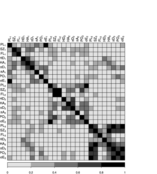
Figure 1: Graphical representation of the absolute correlation matrix of the $26$ predictors for the pyrimidine data. The magnitude of each pairwise correlation is represented by a block in the grayscale image.

Let $\hat{\mathbf{B}}_{1}\in\mathbb{R}^{9}$, $\hat{\mathbf{B}}_{2}\in\mathbb{R}^{9}$ and $\hat{\mathbf{B}}_{3}\in\mathbb{R}^{8}$ denote direction estimates for the three predictor groups, respectively. We next consider the group-wise additive index model

$$Y=G_{1}(Z_{1})+G_{2}(Z_{2})+G_{3}(Z_{3})+\varepsilon,$$

==0pt Pyrimidine data. Estimated coefficients and adjusted $R$-squared values ($\bar{R}^{2}$) from various methods OLS LASSO SCAD MCP gMAVE SgMAVE-LASSO SgMAVE-SCAD SgMAVE-MCP $\mathbf{V}_{1}$: attributes of a substituent at position 1 $\mathrm{PL}_{1}$ $-0.0437$ $0$ $0$ $0$ $0.6240$ $0.5620$ $0.6043$ $0.5896$ $\mathrm{SZ}_{1}$ $0.0435$ $0.0358$ $0$ $0.0586$ $-0.3154$ $-0.3772$ $-0.3336$ $-0.3470$ $\mathrm{FL}_{1}$ $-0.0444$ $-0.0323$ $-0.0216$ $-0.0537$ $0.2890$ $0.3444$ $0.3035$ $0.3198$ $\mathrm{HD}_{1}$ $-0.0249$ $-0.0197$ $-0.0480$ $-0.0273$ $0.1079$ $0.1589$ $0.1288$ $0.1407$ $\mathrm{HA}_{1}$ $0.0139$ $0$ $0.0358$ $0$ $-0.0227$ $0$ $0$ $0$ $\pi\mathrm{D}_{1}$ $0.0083$ $0.0025$ $0.0185$ $0.0207$ $-0.0521$ $-0.0928$ $-0.0898$ $-0.0916$ $\pi\mathrm{A}_{1}$ $0.0122$ $0$ $0.0160$ $0$ $-0.1901$ $-0.1818$ $-0.1985$ $-0.1949$ $\mathrm{PO}_{1}$ $0.0288$ $0.0224$ $0.0291$ $0$ $-0.3498$ $-0.3604$ $-0.3701$ $-0.3711$ $\sigma\mathrm{E}_{1}$ $0.0386$ $0.0080$ $0$ $0$ $-0.5040$ $-0.4756$ $-0.4798$ $-0.4749$ $\mathbf{V}_{2}$: attributes of a substituent at position 2 $\mathrm{PL}_{2}$ $-0.0281$ $0$ $-0.0025$ $0$ $0.6924$ $0.6763$ $0.6894$ $0.6812$ $\mathrm{SZ}_{2}$ $0.0396$ $0.0152$ $0.0324$ $0$ $-0.1058$ $-0.1023$ $-0.0991$ $-0.0849$ $\mathrm{FL}_{2}$ $-0.0430$ $-0.0240$ $-0.0407$ $-0.0179$ $-0.1802$ $-0.2211$ $-0.1904$ $-0.2232$ $\mathrm{HD}_{2}$ $0.0076$ $0$ $0$ $0$ $-0.0982$ $-0.0556$ $-0.0841$ $-0.0574$ $\mathrm{HA}_{2}$ $0.0068$ $0$ $0$ $0$ $0.0402$ $0.0440$ $0.0328$ $0.0494$ $\pi\mathrm{D}_{2}$ $-0.0132$ $0.0100$ $0$ $0$ $0.0663$ $0$ $0.0534$ $0$ $\pi\mathrm{A}_{2}$ $0.0030$ $0$ $0$ $0$ $-0.1654$ $-0.1702$ $-0.1672$ $-0.1770$ $\mathrm{PO}_{2}$ $0.0218$ $0.0145$ $0.0148$ $0.0257$ $-0.3264$ $-0.3575$ $-0.3348$ $-0.3462$ $\sigma\mathrm{E}_{2}$ $0.0176$ $0$ $0$ $0$ $-0.5720$ $-0.5667$ $-0.5722$ $-0.5673$ $\mathbf{V}_{3}$: attributes of a substituent at position 3 $\mathrm{PL}_{3}$ $0.0103$ $0$ $0$ $0$ $-0.0925$ $-0.1599$ $-0.1506$ $-0.1501$ $\mathrm{SZ}_{3}$ $0.0458$ $0.0579$ $0.0955$ $0.0740$ $0.7768$ $0.8369$ $0.9125$ $0.9126$ $\mathrm{FL}_{3}$ $-0.0311$ $-0.0079$ $-0.0309$ $-0.0208$ $-0.1757$ $-0.1957$ $-0.2048$ $-0.2070$ $\mathrm{HD}_{3}$ $-0.0540$ $-0.0424$ $-0.0294$ $-0.0340$ $0.0586$ $0$ $0$ $0$ $\mathrm{HA}_{3}$ $0.0595$ $0$ $0$ $0$ $-0.2928$ $-0.2298$ $-0.2689$ $-0.2667$ $\pi\mathrm{D}_{3}$ $-0.1958$ $-0.0696$ $-0.1620$ $-0.1459$ $-0.3503$ $-0.3490$ $-0.1738$ $-0.1744$ $\mathrm{PO}_{3}$ $0.0696$ $0.0365$ $0.0470$ $0.0623$ $-0.0992$ $0.0080$ $0$ $0$ $\sigma\mathrm{E}_{3}$ $0.0987$ $0.0363$ $0.0864$ $0.0806$ $0.3677$ $0.2468$ $0$ $0$ $\bar{R}^{2}$ $0.8206$ $0.7934$ $0.8311$ $0.8226$ $0.9150$ $0.9241$ $0.9170$ $0.9210$ where $Z_{l}=\hat{\mathbf{B}}_{l}^{\top}\mathbf{V}_{l}$, $l=1,2$ and $3$, are the extracted linear predictors, and $G_{l}(\cdot)$’s are unknown univariate functions. We fit this model by applying the gam function in the publicly available R package mgcv. The adjusted percentages of total deviance explained, namely the adjusted R-squared values, for various methods are summarized in the last row of Table 3.2. Unreported results show that the nonparametric smoothing of all the three predictors yields better performance than the additive model using smoothing of every single predictor, but the improvement is not statistically significant. As we can see, the proposed semi-parametric methods outperform the classical parametric ones as they can provide a mechanism for exploring nonlinear relationships between molecular structure and biological activity.

Figure 2 provides the plots of estimated index functions, using for illustration the shrinkage group-wise MAVE method with the minimax concave penalty (SgMAVE-MCP). From Figures 2(a) and (b), it can be seen that $G_{1}(\cdot)$ has a linear trend, while $G_{2}(\cdot)$ is clearly curved, indicating a nonlinear parabolic dependence of activity on the extracted linear combination of attributes at the second position of substitution. It can also be seen from Figure 2(c) that $G_{3}(\cdot)$ is very complicated, and nonparametric smoothing performs poorly in areas where observations are sparse.

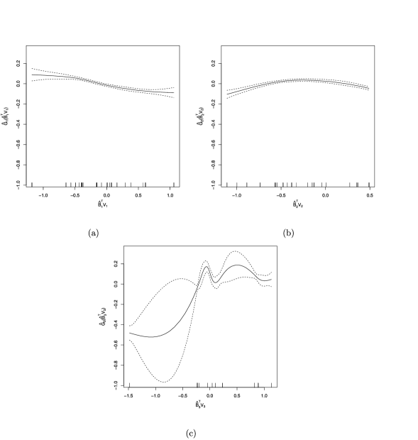
Figure 2: The panels show the estimates of the terms in the group-wise additive index model for the pyrimidine data using for illustration SgMAVE-MCP. The upper left panel, the upper right panel and the lower panel are the smooth functions of the extracted linear predictor in predictor group one, two and three, respectively. The rug plots, along the bottom of each plot, show the values of the predictors of each smooth. Thin plate regression splines were used with smoothing parameters being selected by GCV.

4 Discussion

In this paper, we only provide the convergence rate of the shrinkage group-wise MAVE estimator. It is possible to derive the limiting distribution. However, the limiting distribution is too complicated to be applied for inference. Thus, for the time being, we are frustrated by the lack of a good approximation to the limiting distribution that can be used to set standard errors or to carry out tests on the parameter vector.

As remarked by Knight and Fu [16], attaching standard errors to LASSO-type estimators is nontrivial. They then considered using the residual-based bootstrap method to estimate the sampling distribution of the LASSO estimator in a multiple linear regression. However, Chatterjee and Lahiri [3] showed that the conditional residual bootstrap distribution given the data converges to a random measure; that is, the residual bootstrap estimate of the LASSO distribution is inconsistent. In a subsequent paper, Chatterjee and Lahiri [4] proposed a modified bootstrap method, and showed that it provides a valid approximation to the distribution of the LASSO estimator.

But it is unclear yet whether or not the modified bootstrap method of Chatterjee and Lahiri [4] can be applied to our setting. The situation is complicated by the fact that in semi-parametric multiple-index models we need to take into account the interaction between nonparametric function estimation and shrinkage direction estimation. Work along this line is in progress.

Appendix

We need the following regularity conditions:

1. [(A3)]

2. $E|Y|^{k}<\infty$ and $E\|\mathbf{X}\|_{2}^{k}<\infty$ for some large $k>0$, where $\|\cdot\|_{2}$ denotes the $\ell_{2}$ norm.

3. The density function of $\mathbf{X}$ has a bounded second derivative; $E(\mathbf{X}|\mathbf{B}^{\top}\mathbf{X}=\mathbf{w})$ and $E(\mathbf{X}\mathbf{X}^{\top}|\mathbf{B}^{\top}\mathbf{X}=\mathbf{w})$ have bounded derivatives with respect to $\mathbf{w}$ and $\mathbf{B}$ for $\mathbf{B}$ in a small neighborhood of $\mathbf{B}^{*}$, that is, $\|\mathbf{P}_{\mathbf{B}}-\mathbf{P}_{\mathbf{B}^{*}}\|_{2}\leq\zeta$ for some small $\zeta>0$.

4. The function $E(Y|\mathbf{B}^{\top}\mathbf{X}=\mathbf{w})$ has a bounded and continuous fourth derivative with respect to $\mathbf{w}$ and $\mathbf{B}$ for $\mathbf{B}$ in a small neighborhood of $\mathbf{B}^{*}$.

5. The kernel $K(\cdot)$ is a Gaussian probability density function.

6. $d\leq 3$ and $h\propto n^{-1/(d+4)}$.

7. $\tilde{\mathbf{B}}_{l}=\mathbf{B}_{l}^{*}\mathbf{D}_{l}^{0}+\mathrm{O}_{P}(n^{-1/2})$ and $\tilde{\tilde{\mathbf{B}}}_{l}=\mathbf{B}_{l}^{*}\mathbf{D}_{l}^{0}+\mathrm{O}_{P}(n^{-1/2})$ for some $d_{l}\times d_{l}$ nonsingular matrix $\mathbf{D}_{l}^{0}$ for $l=1,\ldots,g$.

Note that conditions (A1)–(A4) are standard in the literature, see for instance Wang and Xia [28], Xia [32] and Li, Li and Zhu [19]. As shown in Xia [32], the ordinary MAVE estimator is root-$n$ consistent under conditions similar to (A1)–(A5). Consequently, condition (A6) is very reasonable because we can view $\tilde{\mathbf{B}}=\bigoplus_{l=1}^{g}\tilde{\mathbf{B}}_{l}$ as a special case of a general $\tilde{\mathbf{B}}$ in Xia’s proof. If higher order local polynomial smoothing is used, the root-$n$ consistency can also be achieved for $d>3$; see Remark 5.3 in Xia [32]. Nevertheless, in practice models with $d>3$ are not attractive due to the “curse of dimensionality”.

Before we begin the proof, we need to introduce some additional notation. For a positive integer $m$, $\mathbf{0}_{m}$ stands for an $m$-dimensional vector of zeros. For an $m_{1}\times m_{2}$ matrix $\mathbf{A}$, $\operatorname{vec}(\mathbf{A})$ stands for the $m_{1}m_{2}$-dimensional vector obtained by stacking the columns of $\mathbf{A}$. For a diagonal matrix, we get the (generalized) inverse by taking the reciprocal of each nonzero element on the diagonal, leaving the zeros in place, and transposing the resulting matrix.

Let $\hat{\mathbf{B}}_{l}=\operatorname{diag}(\hat{\bm{\alpha}}_{l})\tilde{\tilde{\mathbf{B}}}_{l}$. Then $\hat{\mathbf{B}}=\bigoplus_{l=1}^{g}\hat{\mathbf{B}}_{l}$. Let $\tilde{\tilde{B}}_{lst}$ denote the $(s,t)$th element of $\tilde{\tilde{\mathbf{B}}}_{l}$. Without loss of generality, we assume that $\mathbf{D}_{l}^{0}=\mathbf{I}_{d_{l}}$, and the first $q_{l}$ components of $\mathbf{B}_{l1}^{*}$ are nonzero. For each $l=1,\ldots,g$, we define

$$\mathbf{H}_{l}^{*}=\pmatrix{\operatorname{diag}\bigl{(}\mathbf{B}^{*}_{l1}\bigr{)}\cr\vdots\cr\operatorname{diag}\bigl{(}\mathbf{B}^{*}_{ld_{l}}\bigr{)}}\bigl{\{}\operatorname{diag}\bigl{(}\mathbf{B}^{*}_{l1}\bigr{)}\bigr{\}}^{-1}\quad\mbox{{and}}\quad\tilde{\tilde{\mathbf{H}}}_{l}=\pmatrix{\operatorname{diag}(\tilde{\tilde{\mathbf{B}}}_{l1})\cr\vdots\cr\operatorname{diag}(\tilde{\tilde{\mathbf{B}}}_{ld_{l}})}\bigl{\{}\operatorname{diag}(\tilde{\tilde{\mathbf{B}}}_{l1})\bigr{\}}^{-1},$$

where $\mathbf{B}^{*}_{lt}$ denotes the $t$th column of $\mathbf{B}^{*}_{l}$ and $\tilde{\tilde{\mathbf{B}}}_{lt}$ denotes the $t$th column of $\tilde{\tilde{\mathbf{B}}}_{l}$, $t=1,\ldots,d_{l}$. Let $\mathbf{H}^{*}=\bigoplus_{l=1}^{g}\mathbf{H}_{l}^{*}$ and $\tilde{\tilde{\mathbf{H}}}=\bigoplus_{l=1}^{g}\tilde{\tilde{\mathbf{H}}}_{l}$. By condition (A6), $\|\mathbf{H}^{*}-\tilde{\tilde{\mathbf{H}}}\|_{2}=\mathrm{O}_{P}(n^{-1/2})$.

Proof of Theorem 2.1 We shall concentrate on the optimization problem (5). The proof follows Theorem 1 of Bondell and Li [1] closely. First, we formulate an equivalent optimization problem that is easier to analyze theoretically. To see this, we note that

$$\sum_{i=1}^{n}\sum_{j=1}^{n}\Biggl{\{}y^{j}-{\tilde{a}^{i}}-\sum_{l=1}^{g}{\tilde{\mathbf{b}}}_{l}^{i\top}\tilde{\tilde{\mathbf{B}}}_{l}{\vphantom{\tilde{B}}\!\!}^{\top}\operatorname{diag}\bigl{(}\mathbf{v}_{l}^{j}-\mathbf{v}_{l}^{i}\bigr{)}\bm{\alpha}_{l}\Biggr{\}}^{2}\tilde{w}_{j}^{i}$$

$$\quad=\sum_{i=1}^{n}\sum_{j=1}^{n}\Biggl{[}y^{j}-{\tilde{a}^{i}}-\sum_{l=1}^{g}\bigl{\{}{\tilde{\mathbf{b}}}_{l}^{i\top}\otimes\bigl{(}\mathbf{v}_{l}^{j}-\mathbf{v}_{l}^{i}\bigr{)}^{\top}\bigr{\}}\pmatrix{\operatorname{diag}(\tilde{\tilde{\mathbf{B}}}_{l1})\cr\vdots\cr\operatorname{diag}(\tilde{\tilde{\mathbf{B}}}_{ld_{l}})}\bm{\alpha}_{l}\Biggr{]}^{2}\tilde{w}_{j}^{i}$$

$$\quad=\sum_{i=1}^{n}\sum_{j=1}^{n}\Biggl{[}y^{j}-{\tilde{a}^{i}}-\sum_{l=1}^{g}\bigl{\{}{\tilde{\mathbf{b}}}_{l}^{i\top}\otimes\bigl{(}\mathbf{v}_{l}^{j}-\mathbf{v}_{l}^{i}\bigr{)}^{\top}\bigr{\}}\tilde{\tilde{\mathbf{H}}}_{l}\operatorname{diag}(\tilde{\tilde{\mathbf{B}}}_{l1})\bm{\alpha}_{l}\Biggr{]}^{2}\tilde{w}_{j}^{i}.$$

Suppose that $\{\check{\mathbf{B}}_{l1}=(\check{B}_{l11},\ldots,\check{B}_{lp_{l}1})^{\top}\in\mathbb{R}^{p_{l}},l=1,\ldots,g\}$ is the minimizer of

$$\sum_{i=1}^{n}\sum_{j=1}^{n}\Biggl{[}y^{j}-{\tilde{a}^{i}}-\sum_{l=1}^{g}\bigl{\{}{\tilde{\mathbf{b}}}_{l}^{i\top}\otimes\bigl{(}\mathbf{v}_{l}^{j}-\mathbf{v}_{l}^{i}\bigr{)}^{\top}\bigr{\}}\tilde{\tilde{\mathbf{H}}}_{l}\mathbf{B}_{l1}\Biggr{]}^{2}\tilde{w}_{j}^{i}+\lambda_{n}\sum_{l=1}^{g}\sum_{s=1}^{p_{l}}\frac{|B_{ls1}|}{|\tilde{\tilde{B}}_{ls1}|}$$ (13)

with respect to $\{\mathbf{B}_{l1}=(B_{l11},\ldots,B_{lp_{l}1})^{\top}\in\mathbb{R}^{p_{l}},l=1,\ldots,g\}$. From Definition 2.1, it is easy to see that $\hat{\alpha}_{ls}=(\tilde{\tilde{B}}_{ls1})^{-1}\check{B}_{ls1}$ for all $l=1,\ldots,g$ and $s=1,\ldots,p_{l}$. Further, $\operatorname{vec}({\hat{\mathbf{B}}}_{l})=\tilde{\tilde{\mathbf{H}}}_{l}\check{\mathbf{B}}_{l1}$.

Below we shall describe the details of the proof by breaking it up into two steps. Step I establishes the convergence rate of $\hat{\mathbf{B}}$. Step II shows that $\hat{\mathbf{B}}$ attains sparsity.

Step I. Let $\mathbf{u}=(\mathbf{u}_{1}^{\top},\ldots,\mathbf{u}_{g}^{\top})^{\top}\in\mathbb{R}^{p}$, where $\mathbf{u}_{l}=(u_{l1},\ldots,u_{lp_{l}})^{\top}\in\mathbb{R}^{p_{l}}$ for $l=1,\ldots,g$. Define

$$J_{n}(\mathbf{u})=\lambda_{n}\sum_{l=1}^{g}\sum_{s=1}^{p_{l}}|\tilde{\tilde{B}}_{ls1}|^{-1}\biggl{|}B_{ls1}^{*}+\frac{u_{ls}}{\sqrt{n}}\biggr{|}.$$

Then, we have

$$J_{n}(\mathbf{u})-J_{n}(\mathbf{0}_{p})=\frac{\lambda_{n}}{\sqrt{n}}\sum_{l=1}^{g}\sum_{s=1}^{p_{l}}|\tilde{\tilde{B}}_{ls1}|^{-1}\sqrt{n}\biggl{(}\biggl{|}B_{ls1}^{*}+\frac{u_{ls}}{\sqrt{n}}\biggr{|}-\bigl{|}B_{ls1}^{*}\bigr{|}\biggr{)}.$$

If $u_{ls}=0$, then

$$\frac{\lambda_{n}}{\sqrt{n}}|\tilde{\tilde{B}}_{ls1}|^{-1}\sqrt{n}\biggl{(}\biggl{|}B_{ls1}^{*}+\frac{u_{ls}}{\sqrt{n}}\biggr{|}-\bigl{|}B_{ls1}^{*}\bigr{|}\biggr{)}=0.$$

If $u_{ls}\neq 0$ and $B_{ls1}^{*}\neq 0$, then $|\tilde{\tilde{B}}_{ls1}|^{-1}\rightarrow_{P}|B_{ls1}^{*}|^{-1}$ and

$$\sqrt{n}\biggl{(}\biggl{|}B_{ls1}^{*}+\frac{u_{ls}}{\sqrt{n}}\biggr{|}-\bigl{|}B_{ls1}^{*}\bigr{|}\biggr{)}\rightarrow u_{ls}\times\operatorname{sgn}\bigl{(}B_{ls1}^{*}\bigr{)},$$

where $\operatorname{sgn}(\cdot)$ is the sign function. By Slutsky’s theorem,

$$\frac{\lambda_{n}}{\sqrt{n}}|\tilde{\tilde{B}}_{ls1}|^{-1}\sqrt{n}\biggl{(}\biggl{|}B_{ls1}^{*}+\frac{u_{ls}}{\sqrt{n}}\biggr{|}-\bigl{|}B_{ls1}^{*}\bigr{|}\biggr{)}=\mathrm{o}_{P}\bigl{(}h^{2}\bigr{)}.$$

If $u_{ls}\neq 0$ and $B_{ls1}^{*}=0$, then

$$\frac{\lambda_{n}}{\sqrt{n}}|\tilde{\tilde{B}}_{ls1}|^{-1}\sqrt{n}\biggl{(}\biggl{|}B_{ls1}^{*}+\frac{u_{ls}}{\sqrt{n}}\biggr{|}-\bigl{|}B_{ls1}^{*}\bigr{|}\biggr{)}=\frac{\lambda_{n}}{\sqrt{n}|\tilde{\tilde{B}}_{ls1}|}|u_{ls}|\rightarrow_{P}\infty.$$

Define

$$\Psi_{n}(\mathbf{u})=\sum_{i=1}^{n}\sum_{j=1}^{n}\Biggl{[}y^{j}-{\tilde{a}^{i}}-\sum_{l=1}^{g}\bigl{\{}{\tilde{\mathbf{b}}}_{l}^{i\top}\otimes\bigl{(}\mathbf{v}_{l}^{j}-\mathbf{v}_{l}^{i}\bigr{)}^{\top}\bigr{\}}\tilde{\tilde{\mathbf{H}}}_{l}\biggl{(}\mathbf{B}_{l1}^{*}+\frac{\mathbf{u}_{l}}{\sqrt{n}}\biggr{)}\Biggr{]}^{2}\tilde{w}_{j}^{i}.$$

After some algebra one gets

$$\Psi_{n}(\mathbf{u})-\Psi_{n}(\mathbf{0}_{p})$$

$$\quad=\sum_{i=1}^{n}\sum_{j=1}^{n}\Biggl{[}\sum_{l=1}^{g}\bigl{\{}{\tilde{\mathbf{b}}}_{l}^{i\top}\otimes\bigl{(}\mathbf{v}_{l}^{j}-\mathbf{v}_{l}^{i}\bigr{)}^{\top}\bigr{\}}\tilde{\tilde{\mathbf{H}}}_{l}\frac{\mathbf{u}_{l}}{\sqrt{n}}\Biggr{]}^{2}\tilde{w}_{j}^{i}$$

$$\qquad{}+2\sum_{i=1}^{n}\sum_{j=1}^{n}\Biggl{[}\sum_{l=1}^{g}\bigl{\{}{\tilde{\mathbf{b}}}_{l}^{i\top}\otimes\bigl{(}\mathbf{v}_{l}^{j}-\mathbf{v}_{l}^{i}\bigr{)}^{\top}\bigr{\}}\tilde{\tilde{\mathbf{H}}}_{l}\frac{\mathbf{u}_{l}}{\sqrt{n}}\Biggr{]}$$

$$\phantom{\qquad{}+}{}\times\Biggl{[}\sum_{l=1}^{g}\bigl{\{}{\tilde{\mathbf{b}}}_{l}^{i\top}\otimes\bigl{(}\mathbf{v}_{l}^{j}-\mathbf{v}_{l}^{i}\bigr{)}^{\top}\bigr{\}}\tilde{\tilde{\mathbf{H}}}_{l}\bigl{(}\mathbf{B}_{l1}^{*}-\tilde{\tilde{\mathbf{B}}}_{l1}\bigr{)}\Biggr{]}\tilde{w}_{j}^{i}.$$

Let $\mathbf{v}^{*}=(\mathbf{B}_{11}^{*\top},\ldots,\mathbf{B}_{g1}^{*\top})^{\top}$ and $\tilde{\tilde{\mathbf{v}}}=(\tilde{\tilde{\mathbf{B}}}_{11}{\vphantom{\tilde{B}}\!\!}^{\top},\ldots,\tilde{\tilde{\mathbf{B}}}_{g1}{\vphantom{\tilde{B}}\!\!}^{\top})^{\top}$. Then, we have

$$\Psi_{n}(\mathbf{u})-\Psi_{n}(\mathbf{0}_{p}) = \mathbf{u}^{\top}\tilde{\tilde{\mathbf{H}}}{\vphantom{\tilde{H}}\!\!}^{\top}\Biggl{(}\frac{1}{n}\sum_{i=1}^{n}\sum_{j=1}^{n}\tilde{\mathbf{v}}_{ij}\tilde{\mathbf{v}}_{ij}^{\top}\tilde{w}_{j}^{i}\Biggr{)}\tilde{\tilde{\mathbf{H}}}\mathbf{u}$$

$${}+2\mathbf{u}^{\top}\tilde{\tilde{\mathbf{H}}}{\vphantom{\tilde{H}}\!\!}^{\top}\Biggl{(}\frac{1}{n}\sum_{i=1}^{n}\sum_{j=1}^{n}\tilde{\mathbf{v}}_{ij}\tilde{\mathbf{v}}_{ij}^{\top}\tilde{w}_{j}^{i}\Biggr{)}\tilde{\tilde{\mathbf{H}}}\bigl{\{}\sqrt{n}\bigl{(}\mathbf{v}^{*}-\tilde{\tilde{\mathbf{v}}}\bigr{)}\bigr{\}}$$

$$\equiv T_{1}+T_{2},$$

where $\tilde{\mathbf{v}}_{ij}=(\tilde{\mathbf{v}}_{ij1}^{\top},\ldots,\tilde{\mathbf{v}}_{ijg}^{\top})^{\top}\in\mathbb{R}^{p_{1}d_{1}+\cdots+p_{g}d_{g}}$, $\tilde{\mathbf{v}}_{ijl}={\tilde{\mathbf{b}}_{l}^{i}}\otimes(\mathbf{v}_{l}^{j}-\mathbf{v}_{l}^{i})\in\mathbb{R}^{p_{l}d_{l}}$, $l=1,\ldots,g$.

First, we consider $T_{1}$. Note that

$$T_{1} = \mathbf{u}^{\top}\mathbf{H}^{*\top}\Biggl{(}\frac{1}{n}\sum_{i=1}^{n}\sum_{j=1}^{n}\tilde{\mathbf{v}}_{ij}\tilde{\mathbf{v}}_{ij}^{\top}\tilde{w}_{j}^{i}\Biggr{)}\mathbf{H}^{*}\mathbf{u}$$

$${}+\mathbf{u}^{\top}\mathbf{H}^{*\top}\Biggl{(}\frac{1}{n}\sum_{i=1}^{n}\sum_{j=1}^{n}\tilde{\mathbf{v}}_{ij}\tilde{\mathbf{v}}_{ij}^{\top}\tilde{w}_{j}^{i}\Biggr{)}\bigl{(}\tilde{\tilde{\mathbf{H}}}-\mathbf{H}^{*}\bigr{)}\mathbf{u}$$

$${}+\mathbf{u}^{\top}\bigl{(}\tilde{\tilde{\mathbf{H}}}-\mathbf{H}^{*}\bigr{)}^{\top}\Biggl{(}\frac{1}{n}\sum_{i=1}^{n}\sum_{j=1}^{n}\tilde{\mathbf{v}}_{ij}\tilde{\mathbf{v}}_{ij}^{\top}\tilde{w}_{j}^{i}\Biggr{)}\mathbf{H}^{*}\mathbf{u}$$

$${}+\mathbf{u}^{\top}\bigl{(}\tilde{\tilde{\mathbf{H}}}-\mathbf{H}^{*}\bigr{)}^{\top}\Biggl{(}\frac{1}{n}\sum_{i=1}^{n}\sum_{j=1}^{n}\tilde{\mathbf{v}}_{ij}\tilde{\mathbf{v}}_{ij}^{\top}\tilde{w}_{j}^{i}\Biggr{)}\bigl{(}\tilde{\tilde{\mathbf{H}}}-\mathbf{H}^{*}\bigr{)}\mathbf{u}$$

$$\equiv T_{11}+T_{12}+T_{13}+T_{14}.$$

By Lemma 4 in Wang and Xia [28],

$$\frac{1}{n}\sum_{i=1}^{n}\sum_{j=1}^{n}\tilde{\mathbf{v}}_{ij}\tilde{\mathbf{v}}_{ij}^{\top}\tilde{w}_{j}^{i}=\bm{\Delta}+\mathrm{o}_{P}(1),$$

where $\bm{\Delta}$ is a nonnegative definite matrix. Hence, we obtain

$$T_{11}=\mathrm{O}_{P}(1),\qquad T_{12}=\mathrm{O}_{P}\bigl{(}n^{-1/2}\bigr{)},\qquad T_{13}=\mathrm{O}_{P}\bigl{(}n^{-1/2}\bigr{)}\quad\mbox{and}\quad T_{14}=\mathrm{O}_{P}\bigl{(}n^{-1}\bigr{)}.$$

Next, we consider $T_{2}$. Note that $\tilde{\tilde{\mathbf{v}}}=\mathbf{v}^{*}+\mathrm{O}_{P}(n^{-1/2})$ and

$$T_{2} = 2\mathbf{u}^{\top}\mathbf{H}^{*\top}\Biggl{(}\frac{1}{n}\sum_{i=1}^{n}\sum_{j=1}^{n}\tilde{\mathbf{v}}_{ij}\tilde{\mathbf{v}}_{ij}^{\top}\tilde{w}_{j}^{i}\Biggr{)}\mathbf{H}^{*}\bigl{\{}\sqrt{n}\bigl{(}\mathbf{v}^{*}-\tilde{\tilde{\mathbf{v}}}\bigr{)}\bigr{\}}$$

$${}+2\mathbf{u}^{\top}\mathbf{H}^{*}\Biggl{(}\frac{1}{n}\sum_{i=1}^{n}\sum_{j=1}^{n}\tilde{\mathbf{v}}_{ij}\tilde{\mathbf{v}}_{ij}^{\top}\tilde{w}_{j}^{i}\Biggr{)}\bigl{(}\tilde{\tilde{\mathbf{H}}}-\mathbf{H}^{*}\bigr{)}\bigl{\{}\sqrt{n}\bigl{(}\mathbf{v}^{*}-\tilde{\tilde{\mathbf{v}}}\bigr{)}\bigr{\}}$$

$${}+2\mathbf{u}^{\top}\bigl{(}\tilde{\tilde{\mathbf{H}}}-\mathbf{H}^{*}\bigr{)}^{\top}\Biggl{(}\frac{1}{n}\sum_{i=1}^{n}\sum_{j=1}^{n}\tilde{\mathbf{v}}_{ij}\tilde{\mathbf{v}}_{ij}^{\top}\tilde{w}_{j}^{i}\Biggr{)}\mathbf{H}^{*}\bigl{\{}\sqrt{n}\bigl{(}\mathbf{v}^{*}-\tilde{\tilde{\mathbf{v}}}\bigr{)}\bigr{\}}$$

$${}+2\mathbf{u}^{\top}\bigl{(}\tilde{\tilde{\mathbf{H}}}-\mathbf{H}^{*}\bigr{)}^{\top}\Biggl{(}\frac{1}{n}\sum_{i=1}^{n}\sum_{j=1}^{n}\tilde{\mathbf{v}}_{ij}\tilde{\mathbf{v}}_{ij}^{\top}\tilde{w}_{j}^{i}\Biggr{)}\bigl{(}\tilde{\tilde{\mathbf{H}}}-\mathbf{H}^{*}\bigr{)}\bigl{\{}\sqrt{n}\bigl{(}\mathbf{v}^{*}-\tilde{\tilde{\mathbf{v}}}\bigr{)}\bigr{\}}$$

$$\equiv T_{21}+T_{22}+T_{23}+T_{24}.$$

Thus, we arrive at

$$T_{21}=\mathrm{O}_{P}(1),\qquad T_{22}=\mathrm{O}_{P}\bigl{(}n^{-1/2}\bigr{)},\qquad T_{23}=\mathrm{O}_{P}\bigl{(}n^{-1/2}\bigr{)}\quad\mbox{and}\quad T_{24}=\mathrm{O}_{P}\bigl{(}n^{-1}\bigr{)}.$$

Let $L_{n}(\mathbf{u})=\Psi_{n}(\mathbf{u})+J_{n}(\mathbf{u})$. If $u_{ls}\neq 0$ for some $l\in\{1,\ldots,g\}$ and $s\in\{q_{l}+1,\ldots,p_{l}\}$, then $L_{n}(\mathbf{u})-L_{n}(\mathbf{0}_{p})\rightarrow_{P}\infty>0$. So we assume in the sequel that $\mathbf{u}\in\mathcal{U}$, where

$$\mathcal{U}=\bigl{\{}\mathbf{u}\in\mathbb{R}^{p}:u_{ls}=0\mbox{ for all }l=1,\ldots,g\mbox{ and }s=q_{l}+1,\ldots,p_{l}\bigr{\}}.$$

It follows that $J_{n}(\mathbf{u})-J_{n}(\mathbf{0}_{p})=\mathrm{o}_{P}(h^{2})$ for any $\mathbf{u}\in\mathcal{U}$. Let $\mathbf{u}\in\mathcal{U}$.

We consider the problem of minimizing $L_{n}(\mathbf{u})$ over $\mathcal{U}$. Because $nh^{4}\rightarrow\infty$, we obtain

$$L_{n}(\mathbf{u})-L_{n}(\mathbf{0}_{p})=T_{11}+T_{21}+\mathrm{o}_{P}\bigl{(}h^{2}\bigr{)}.$$

Let $(\mathbf{B}_{l}^{*},\mathbf{A}_{l}^{*})$ be an orthogonal matrix. Let $\mathbf{C}=\bigoplus_{l=1}^{g}\{\mathbf{I}_{d_{l}}\otimes(\mathbf{B}_{l}^{*},\mathbf{A}_{l}^{*})\}$. Then, according to Lemma 4 of Wang and Xia [28], the long version, there exists a $(\sum_{l=1}^{g}d_{l}p_{l})\times(\sum_{l=1}^{g}d_{l}p_{l})$ permutation matrix $\bm{\Pi}=\bigoplus_{l=1}^{g}\bm{\Pi}_{l}$ such that

$$\frac{1}{n}\sum_{i=1}^{n}\sum_{j=1}^{n}\tilde{\mathbf{v}}_{ij}\tilde{\mathbf{v}}_{ij}^{\top}\tilde{w}_{j}^{i}=\mathbf{C}\bm{\Pi}\pmatrix{\bm{\Delta}_{11n}&\bm{\Delta}_{12n}\cr\bm{\Delta}_{21n}&\bm{\Delta}_{22n}}(\mathbf{C}\bm{\Pi})^{\top}+\mathrm{o}_{P}\bigl{(}h^{2}\bigr{)},$$

where $h^{-2}\bm{\Delta}_{11n}\rightarrow_{P}\bm{\Delta}_{11}$, $h^{-2}\bm{\Delta}_{12n}\rightarrow_{P}\bm{\Delta}_{12}$, $h^{-2}\bm{\Delta}_{21n}\rightarrow_{P}\bm{\Delta}_{21}$ and $\bm{\Delta}_{22n}\rightarrow_{P}\bm{\Delta}_{22}$. Moreover, both $\bm{\Delta}_{11}$ and $\bm{\Delta}_{22}$ are positive definite.

Write $\mathbf{C}\bm{\Pi}=(\mathbf{D}_{1},\mathbf{D}_{2})$ with $\mathbf{D}_{1}$ being of order $(\sum_{l=1}^{g}d_{l}p_{l})\times(\sum_{l=1}^{g}d_{l}^{2})$. Let $\mathbf{z}_{1}=\mathbf{D}_{1}^{\top}\mathbf{H}^{*}\mathbf{u}$ and $\mathbf{z}_{2}=\mathbf{D}_{2}^{\top}\mathbf{H}^{*}\mathbf{u}$. Write $\mathbf{z}=(\mathbf{z}_{1}^{\top},\mathbf{z}_{2}^{\top})^{\top}$. Now consider the function

$$G_{n}(\mathbf{z}) = \mathbf{z}^{\top}\pmatrix{\bm{\Delta}_{11n}&\bm{\Delta}_{12n}\cr\bm{\Delta}_{21n}&\bm{\Delta}_{22n}}\mathbf{z}$$

$${}+2\mathbf{z}^{\top}\pmatrix{\bm{\Delta}_{11n}&\bm{\Delta}_{12n}\cr\bm{\Delta}_{21n}&\bm{\Delta}_{22n}}(\mathbf{C}\bm{\Pi})^{\top}\mathbf{H}^{*}\bigl{\{}\sqrt{n}\bigl{(}\mathbf{v}^{*}-\tilde{\tilde{\mathbf{v}}}\bigr{)}\bigr{\}}+\mathrm{o}_{P}\bigl{(}h^{2}\bigr{)}.$$

Denote $\check{\mathbf{z}}=(\check{\mathbf{z}}_{1}^{\top},\check{\mathbf{z}}_{2}^{\top})^{\top}$ the minimizer of $G_{n}(\mathbf{z})$. It turns out that the conditions of Theorem 1 of Radchenko [22] are satisfied and, consequently, we have $\check{\mathbf{z}}_{1}=\mathrm{O}_{P}(1)$ and $\check{\mathbf{z}}_{2}=\mathrm{O}_{P}(1)$. Over $\mathcal{U}$, because $\mathbf{u}=(\mathbf{H}^{*\top}\mathbf{H}^{*})^{-1}\mathbf{H}^{*\top}(\mathbf{D}_{1},\mathbf{D}_{2})\mathbf{z}$, we have $\check{\mathbf{u}}=\mathrm{O}_{P}(1)$. We thus conclude that there exists a minimizer $\{\check{\mathbf{B}}_{l1},l=1,\ldots,g\}$ of (13) such that $\|\check{\mathbf{B}}_{l1}-\mathbf{B}_{l1}^{*}\|_{2}=\mathrm{O}_{P}(n^{-1/2})$ for all $l=1,\ldots,g$.

Since $\operatorname{vec}({{\mathbf{B}}}_{l}^{*})={\mathbf{H}}_{l}^{*}{\mathbf{B}}_{l1}^{*}$ and $\operatorname{vec}({\hat{\mathbf{B}}}_{l})=\tilde{\tilde{\mathbf{H}}}_{l}\check{\mathbf{B}}_{l1}$, by triangular inequality we have

$$\bigl{\|}\operatorname{vec}(\hat{\mathbf{B}}_{l})-\operatorname{vec}\bigl{(}\mathbf{B}_{l}^{*}\bigr{)}\bigr{\|}_{2}\leq\bigl{\|}\operatorname{vec}\bigl{(}{\mathbf{H}}_{l}^{*}\check{\mathbf{B}}_{l1}\bigr{)}-\operatorname{vec}\bigl{(}\mathbf{H}_{l}^{*}\mathbf{B}_{l1}^{*}\bigr{)}\bigr{\|}_{2}+\bigl{\|}\operatorname{vec}(\tilde{\tilde{\mathbf{H}}}_{l}\check{\mathbf{B}}_{l1})-\operatorname{vec}\bigl{(}{\mathbf{H}}_{l}^{*}\check{\mathbf{B}}_{l1}\bigr{)}\bigr{\|}_{2}.$$

Therefore, $\|\hat{\mathbf{B}}_{l}-\mathbf{B}_{l}^{*}\|_{2}=\mathrm{O}_{P}(n^{-1/2})$ for all $l=1,\ldots,g$.

Step II. We show the variable selection consistency. Write $\mathcal{A}_{l}=\mathcal{I}(\mathbf{B}^{*}_{l})$ and $\mathcal{A}_{nl}=\mathcal{I}(\hat{\mathbf{B}}_{l})$. For any $s\in\bigcup_{l=1}^{g}\mathcal{A}_{l}$, that is, $s\in\mathcal{A}_{l}$ for some $l$, the estimation consistency result indicates that $\hat{\alpha}_{ls}\rightarrow_{P}1$. Thus, $P(s\in\bigcup_{l=1}^{g}\mathcal{A}_{nl})\rightarrow 1$. It then suffices to show that for any $s^{\prime}\notin\bigcup_{l=1}^{g}\mathcal{A}_{l}$, $P(s^{\prime}\in\bigcup_{l=1}^{g}\mathcal{A}_{nl})\rightarrow 0$. Consider the event $\{s^{\prime}\in\mathcal{A}_{nl}\}$. By standard Karush–Kuhn–Tucker conditions for optimality, we know that

$$\frac{2}{\sqrt{n}}\sum_{i=1}^{n}\sum_{j=1}^{n}\Biggl{[}y^{j}-{\tilde{a}^{i}}-\sum_{l=1}^{g}\bigl{\{}{\tilde{\mathbf{b}}}_{l}^{i\top}\otimes\bigl{(}\mathbf{v}_{l}^{j}-\mathbf{v}_{l}^{i}\bigr{)}^{\top}\bigr{\}}\tilde{\tilde{\mathbf{H}}}_{l}\check{\mathbf{B}}_{l1}\Biggr{]}$$

$$\quad{}\times\bigl{[}\bigl{\{}{\tilde{\mathbf{b}}}_{l}^{i\top}\otimes\bigl{(}\mathbf{v}_{l}^{j}-\mathbf{v}_{l}^{i}\bigr{)}^{\top}\bigr{\}}\tilde{\tilde{\mathbf{H}}}_{l}\mathbf{e}_{ls^{\prime}}\bigr{]}\times\tilde{w}_{j}^{i}=|\tilde{\tilde{B}}_{ls^{\prime}1}|^{-1}\operatorname{sgn}(\check{B}_{ls^{\prime}1})\frac{\lambda_{n}}{\sqrt{n}},$$

where $\mathbf{e}_{ls^{\prime}}\in\mathbb{R}^{p_{l}}$ is the vector containing a 1 in the $s^{\prime}$th position and zeros elsewhere. Note that

$$|\tilde{\tilde{B}}_{ls^{\prime}1}|^{-1}\frac{\lambda_{n}}{\sqrt{n}}=\frac{\lambda_{n}}{\sqrt{n}|\tilde{\tilde{B}}_{ls^{\prime}1}|}\rightarrow_{P}\infty$$

and

$$\frac{2}{\sqrt{n}}\sum_{i=1}^{n}\sum_{j=1}^{n}\Biggl{[}y^{j}-{\tilde{a}^{i}}-\sum_{l=1}^{g}\bigl{\{}{\tilde{\mathbf{b}}}_{l}^{i\top}\otimes\bigl{(}\mathbf{v}_{l}^{j}-\mathbf{v}_{l}^{i}\bigr{)}^{\top}\bigr{\}}\tilde{\tilde{\mathbf{H}}}_{l}\check{\mathbf{B}}_{l1}\Biggr{]}$$

$$\quad{}\times\bigl{[}\bigl{\{}{\tilde{\mathbf{b}}}_{l}^{i\top}\otimes\bigl{(}\mathbf{v}_{l}^{j}-\mathbf{v}_{l}^{i}\bigr{)}^{\top}\bigr{\}}\tilde{\tilde{\mathbf{H}}}_{l}\mathbf{e}_{ls^{\prime}}\bigr{]}\times\tilde{w}_{j}^{i}=\mathrm{O}_{P}(1).$$

Thus, we obtain

$$P\Biggl{(}s^{\prime}\in\bigcup_{l=1}^{g}\mathcal{A}_{nl}\Biggr{)}\leq\sum_{l=1}^{g}P\bigl{(}s^{\prime}\in\mathcal{A}_{nl}\bigr{)}\rightarrow 0.$$

The proof is complete.

Proof of Theorem 2.2 According to whether the fitted model $\mathcal{M}_{\lambda}$ is under-fitted, correctly fitted or over-fitted, we can divide $\mathbb{R}^{+}=[0,\infty)$ into three disjoint parts:

$$\Omega_{-}=\{\lambda:\mathcal{M}_{\lambda}\nsupseteq\mathcal{M}_{T}\},\qquad\Omega_{0}=\{\lambda:\mathcal{M}_{\lambda}=\mathcal{M}_{T}\}$$

and

$$\Omega_{+}=\{\lambda:\mathcal{M}_{\lambda}\supseteq\mathcal{M}_{T},\mathcal{M}_{\lambda}\neq\mathcal{M}_{T}\}.$$

Further, we assume a reference sequence of tuning parameters, $\{\lambda_{n}\}_{n=1}^{\infty}$, which satisfies the conditions in Theorem 2.1. Clearly, $\check{\mathbf{B}}_{l1}=\mathbf{B}_{l1}^{*}+\mathrm{O}_{P}(n^{-1/2})$ and $P(\mathcal{M}_{\lambda_{n}}=\mathcal{M}_{T})\rightarrow 1$.

We write $\bm{\alpha}=(\bm{\alpha}_{1}^{\top},\ldots,\bm{\alpha}_{g}^{\top})^{\top}\equiv(\alpha_{1},\ldots,\alpha_{p})^{\top}\in\mathbb{R}^{p}$ and define

$$\operatorname{RSS}_{\mathcal{M}} = \min_{\bm{\alpha}\in\mathcal{S}_{\mathcal{M}}}\sum_{i=1}^{n}\sum_{j=1}^{n}\Biggl{\{}y^{j}-{\tilde{a}^{i}}-\sum_{l=1}^{g}{\tilde{\mathbf{b}}}_{l}^{i\top}\tilde{\tilde{\mathbf{B}}}_{l}{\vphantom{\tilde{B}}\!\!}^{\top}\operatorname{diag}\bigl{(}\mathbf{v}_{l}^{j}-\mathbf{v}_{l}^{i}\bigr{)}\bm{\alpha}_{l}\Biggr{\}}^{2}\tilde{w}_{j}^{i}$$

$$\equiv \min_{\bm{\alpha}\in\mathcal{S}_{\mathcal{M}}}\sum_{i=1}^{n}\sum_{j=1}^{n}\Biggl{[}y^{j}-{\tilde{a}^{i}}-\sum_{l=1}^{g}\bigl{\{}{\tilde{\mathbf{b}}}_{l}^{i\top}\otimes\bigl{(}\mathbf{v}_{l}^{j}-\mathbf{v}_{l}^{i}\bigr{)}^{\top}\bigr{\}}\tilde{\tilde{\mathbf{H}}}_{l}\operatorname{diag}(\tilde{\tilde{\mathbf{B}}}_{l1})\bm{\alpha}_{l}\Biggr{]}^{2}\tilde{w}_{j}^{i},$$

where $\mathcal{S}_{\mathcal{M}}=\{\mathbf{w}=(w_{1},\ldots,w_{p})^{\top}\in\mathbb{R}^{p}:w_{s}=0,s\notin\mathcal{M}\}$.

For a generic model $\mathcal{M}$, let $\{\breve{\mathbf{B}}_{11}(\mathcal{M}),\ldots,\breve{\mathbf{B}}_{g1}(\mathcal{M})\}$ be the minimizer of

$$\sum_{i=1}^{n}\sum_{j=1}^{n}\Biggl{[}y^{j}-{\tilde{a}^{i}}-\sum_{l=1}^{g}\bigl{\{}{\tilde{\mathbf{b}}}_{l}^{i\top}\otimes\bigl{(}\mathbf{v}_{l}^{j}-\mathbf{v}_{l}^{i}\bigr{)}^{\top}\bigr{\}}\tilde{\tilde{\mathbf{H}}}_{l}\mathbf{B}_{l1}\Biggr{]}^{2}\tilde{w}_{j}^{i}$$

with respect to $(\mathbf{B}_{11}^{\top},\ldots,\mathbf{B}_{g1}^{\top})^{\top}\in\mathcal{S}_{\mathcal{M}}$. Then, we have

$$\operatorname{RSS}_{\mathcal{M}}=\sum_{i=1}^{n}\sum_{j=1}^{n}\Biggl{[}y^{j}-{\tilde{a}^{i}}-\sum_{l=1}^{g}\bigl{\{}{\tilde{\mathbf{b}}}_{l}^{i\top}\otimes\bigl{(}\mathbf{v}_{l}^{j}-\mathbf{v}_{l}^{i}\bigr{)}^{\top}\bigr{\}}\tilde{\tilde{\mathbf{H}}}_{l}\breve{\mathbf{B}}_{l1}\Biggr{]}^{2}\tilde{w}_{j}^{i}.$$

Further, for the full model $\mathcal{M}_{F}$, $\breve{\mathbf{B}}_{l1}(\mathcal{M}_{F})=\tilde{\tilde{\mathbf{B}}}_{l1}$ for all $l=1,\ldots,g$.

We first consider under-fitted models, that is, $\mathcal{M}_{\lambda}\nsupseteq\mathcal{M}_{T}$. Note that

$$\inf_{\lambda\in\Omega_{-}}\operatorname{RSS}_{\lambda}-\operatorname{RSS}_{\lambda_{n}}\geq\inf_{\lambda\in\Omega_{-}}\operatorname{RSS}_{\mathcal{M}_{\lambda}}-\operatorname{RSS}_{\lambda_{n}}\geq\min_{\mathcal{M}\nsupseteq\mathcal{M}_{T}}\operatorname{RSS}_{\mathcal{M}}-\operatorname{RSS}_{\lambda_{n}}.$$

By definition, we know that

$$\operatorname{RSS}_{\mathcal{M}}-\operatorname{RSS}_{\mathcal{M}_{F}} = \sum_{i=1}^{n}\sum_{j=1}^{n}\Biggl{[}y^{j}-{\tilde{a}^{i}}-\sum_{l=1}^{g}\bigl{\{}{\tilde{\mathbf{b}}}_{l}^{i\top}\otimes\bigl{(}\mathbf{v}_{l}^{j}-\mathbf{v}_{l}^{i}\bigr{)}^{\top}\bigr{\}}\tilde{\tilde{\mathbf{H}}}_{l}\breve{\mathbf{B}}_{l1}(\mathcal{M})\Biggr{]}^{2}\tilde{w}_{j}^{i}$$

$${}-\sum_{i=1}^{n}\sum_{j=1}^{n}\Biggl{[}y^{j}-{\tilde{a}^{i}}-\sum_{l=1}^{g}\bigl{\{}{\tilde{\mathbf{b}}}_{l}^{i\top}\otimes\bigl{(}\mathbf{v}_{l}^{j}-\mathbf{v}_{l}^{i}\bigr{)}^{\top}\bigr{\}}\tilde{\tilde{\mathbf{H}}}_{l}\tilde{\tilde{\mathbf{B}}}_{l1}\Biggr{]}^{2}\tilde{w}_{j}^{i}$$

$$= \sum_{i=1}^{n}\sum_{j=1}^{n}\Biggl{[}\sum_{l=1}^{g}\bigl{\{}{\tilde{\mathbf{b}}}_{l}^{i\top}\otimes\bigl{(}\mathbf{v}_{l}^{j}-\mathbf{v}_{l}^{i}\bigr{)}^{\top}\bigr{\}}\tilde{\tilde{\mathbf{H}}}_{l}\bigl{\{}\breve{\mathbf{B}}_{l1}(\mathcal{M})-\tilde{\tilde{\mathbf{B}}}_{l1}\bigr{\}}\Biggr{]}^{2}\tilde{w}_{j}^{i}.$$

According to Lemma 4 of Wang and Xia [28], there exists some constant $\kappa>0$ such that, for any $\mathcal{M}\nsupseteq\mathcal{M}_{T}$,

$$\operatorname{RSS}_{\mathcal{M}}-\operatorname{RSS}_{\mathcal{M}_{F}}\geq\kappa nh^{2}$$

with probability tending to 1. Since $\log(1+x)\geq\min\{0.5x,\log(2)\}$ for any $x>0$, we have

$$\log(\operatorname{RSS}_{\mathcal{M}})-\log(\operatorname{RSS}_{\mathcal{M}_{F}}) = \log\biggl{(}1+\frac{\operatorname{RSS}_{\mathcal{M}}-\operatorname{RSS}_{\mathcal{M}_{F}}}{\operatorname{RSS}_{\mathcal{M}_{F}}}\biggr{)}$$

$$\geq \min\biggl{\{}\log(2),\frac{\operatorname{RSS}_{\mathcal{M}}-\operatorname{RSS}_{\mathcal{M}_{F}}}{2\operatorname{RSS}_{\mathcal{M}_{F}}}\biggr{\}}.$$

Following an argument similar to the one used in the proof of Lemma 1 of Xia et al. [34], one can show that $n^{-1}\operatorname{RSS}_{\mathcal{M}_{F}}\rightarrow_{P}\sigma^{2}$ for some $\sigma>0$. This, together with $n^{-1}\log(n)=\mathrm{o}(h^{2})$, yields that

$$P\Bigl{\{}\min_{\mathcal{M}\nsupseteq\mathcal{M}_{T}}\operatorname{BIC}_{\mathcal{M}}-\operatorname{BIC}_{\mathcal{M}_{F}}+\,\mathrm{o}_{P}\bigl{(}h^{2}\bigr{)}>0\Bigr{\}}\rightarrow 1.$$

Because $\tilde{\tilde{\mathbf{B}}}_{l1}=\mathbf{B}_{l1}^{*}+\mathrm{O}_{P}(n^{-1/2})$ and $\check{\mathbf{B}}_{l1}=\mathbf{B}_{l1}^{*}+\mathrm{O}_{P}(n^{-1/2})$, we obtain

$$\operatorname{RSS}_{\lambda_{n}}-\operatorname{RSS}_{\mathcal{M}_{F}}=\mathrm{O}_{P}\biggl{(}\frac{1}{n}\biggr{)}=\mathrm{o}_{P}\bigl{(}h^{2}\bigr{)}.$$

Thus, we have

$$P\Bigl{(}\inf_{\lambda\in\Omega_{-}}\operatorname{BIC}_{\lambda}-\operatorname{BIC}_{\lambda_{n}}>0\Bigr{)} \geq P\Bigl{(}\inf_{\mathcal{M}\nsupseteq\mathcal{M}_{T}}\operatorname{BIC}_{\mathcal{M}}-\operatorname{BIC}_{\mathcal{M}_{F}}+\operatorname{BIC}_{\mathcal{M}_{F}}-\operatorname{BIC}_{\lambda_{n}}>0\Bigr{)}$$

$$\rightarrow 1.$$

Next, we consider over-fitted models, that is, $\mathcal{M}_{\lambda}\supseteq\mathcal{M}_{T}$ but $\mathcal{M}_{\lambda}\neq\mathcal{M}_{T}$. Observe that

$$\inf_{\lambda\in\Omega_{+}}\operatorname{RSS}_{\lambda}-\operatorname{RSS}_{\lambda_{n}}\geq\inf_{\lambda\in\Omega_{+}}\operatorname{RSS}_{\mathcal{M}_{\lambda}}-\operatorname{RSS}_{\lambda_{n}}\geq\min_{\mathcal{M}\supseteq\mathcal{M}_{T},\mathcal{M}\neq\mathcal{M}_{T}}\operatorname{RSS}_{\mathcal{M}}-\operatorname{RSS}_{\lambda_{n}}.$$

For a generic model $\mathcal{M}$, if $\mathcal{M}\supseteq\mathcal{M}_{T}$, then one can show that

$$\operatorname{RSS}_{\mathcal{M}}=\operatorname{RSS}_{\mathcal{M}_{F}}+\mathrm{O}_{P}\biggl{(}\frac{1}{n}\biggr{)}.$$

Because $\operatorname{RSS}_{\mathcal{M}_{F}}-\operatorname{RSS}_{\lambda_{n}}=\mathrm{O}_{P}(n^{-1})$, it follows that

$$\min_{\mathcal{M}\supseteq\mathcal{M}_{T},\mathcal{M}\neq\mathcal{M}_{T}}\operatorname{RSS}_{\mathcal{M}}-\operatorname{RSS}_{\lambda_{n}}=\mathrm{O}_{P}\biggl{(}\frac{1}{n}\biggr{)}.$$

Then, with probability tending to 1, we have

$$\inf_{\lambda\in\Omega_{+}}\operatorname{RSS}_{\lambda}-\operatorname{RSS}_{\lambda_{n}}+\frac{\log(n)}{n}>0.$$

As a consequence,

$$P\Bigl{(}\inf_{\lambda\in\Omega_{+}}\operatorname{BIC}_{\lambda}-\operatorname{BIC}_{\lambda_{n}}>0\Bigr{)}\geq P\biggl{(}\inf_{\lambda\in\Omega_{+}}\operatorname{RSS}_{\lambda}-\operatorname{RSS}_{\lambda_{n}}+\frac{\log(n)}{n}>0\biggr{)}\rightarrow 1.$$

Combining, the proof is complete.

References

• [1] {barticle}[mr] \bauthor\bsnmBondell,ย \bfnmHowardย D.\binitsH.D. &\bauthor\bsnmLi,ย \bfnmLexin\binitsL. (\byear2009). \btitleShrinkage inverse regression estimation for model-free variable selection. \bjournalJ. R. Stat. Soc. Ser. B Stat. Methodol. \bvolume71 \bpages287โ€“299. \biddoi=10.1111/j.1467-9868.2008.00686.x, issn=1369-7412, mr=2655534 \bptokimsref\endbibitem
• [2] {barticle}[mr] \bauthor\bsnmBreheny,ย \bfnmPatrick\binitsP. &\bauthor\bsnmHuang,ย \bfnmJian\binitsJ. (\byear2011). \btitleCoordinate descent algorithms for nonconvex penalized regression, with applications to biological feature selection. \bjournalAnn. Appl. Stat. \bvolume5 \bpages232โ€“253. \biddoi=10.1214/10-AOAS388, issn=1932-6157, mr=2810396 \bptokimsref\endbibitem
• [3] {barticle}[mr] \bauthor\bsnmChatterjee,ย \bfnmA.\binitsA. &\bauthor\bsnmLahiri,ย \bfnmS.ย N.\binitsS.N. (\byear2010). \btitleAsymptotic properties of the residual bootstrap for Lasso estimators. \bjournalProc. Amer. Math. Soc. \bvolume138 \bpages4497โ€“4509. \biddoi=10.1090/S0002-9939-2010-10474-4, issn=0002-9939, mr=2680074 \bptokimsref\endbibitem
• [4] {barticle}[mr] \bauthor\bsnmChatterjee,ย \bfnmA.\binitsA. &\bauthor\bsnmLahiri,ย \bfnmS.ย N.\binitsS.N. (\byear2011). \btitleBootstrapping lasso estimators. \bjournalJ. Amer. Statist. Assoc. \bvolume106 \bpages608โ€“625. \biddoi=10.1198/jasa.2011.tm10159, issn=0162-1459, mr=2847974 \bptokimsref\endbibitem
• [5] {barticle}[mr] \bauthor\bsnmChen,ย \bfnmXin\binitsX., \bauthor\bsnmZou,ย \bfnmChangliang\binitsC. &\bauthor\bsnmCook,ย \bfnmR.ย Dennis\binitsR.D. (\byear2010). \btitleCoordinate-independent sparse sufficient dimension reduction and variable selection. \bjournalAnn. Statist. \bvolume38 \bpages3696โ€“3723. \biddoi=10.1214/10-AOS826, issn=0090-5364, mr=2766865 \bptokimsref\endbibitem
• [6] {bbook}[mr] \bauthor\bsnmCook,ย \bfnmR.ย Dennis\binitsR.D. (\byear1998). \btitleRegression Graphics: Ideas for Studying Regressions Through Graphics. \bseriesWiley Series in Probability and Statistics: Probability and Statistics. \blocationNew York: \bpublisherWiley. \biddoi=10.1002/9780470316931, mr=1645673 \bptokimsref\endbibitem
• [7] {barticle}[mr] \bauthor\bsnmCook,ย \bfnmR.ย Dennis\binitsR.D. (\byear2004). \btitleTesting predictor contributions in sufficient dimension reduction. \bjournalAnn. Statist. \bvolume32 \bpages1062โ€“1092. \biddoi=10.1214/009053604000000292, issn=0090-5364, mr=2065198 \bptokimsref\endbibitem
• [8] {barticle}[mr] \bauthor\bsnmCook,ย \bfnmR.ย Dennis\binitsR.D. &\bauthor\bsnmLi,ย \bfnmBing\binitsB. (\byear2002). \btitleDimension reduction for conditional mean in regression. \bjournalAnn. Statist. \bvolume30 \bpages455โ€“474. \biddoi=10.1214/aos/1021379861, issn=0090-5364, mr=1902895 \bptokimsref\endbibitem
• [9] {barticle}[mr] \bauthor\bsnmCook,ย \bfnmR.ย Dennis\binitsR.D. &\bauthor\bsnmNi,ย \bfnmLiqiang\binitsL. (\byear2005). \btitleSufficient dimension reduction via inverse regression: A minimum discrepancy approach. \bjournalJ. Amer. Statist. Assoc. \bvolume100 \bpages410โ€“428. \biddoi=10.1198/016214504000001501, issn=0162-1459, mr=2160547 \bptokimsref\endbibitem
• [10] {barticle}[author] \bauthor\bsnmCook,ย \bfnmR.D.\binitsR.D. &\bauthor\bsnmWeisberg,ย \bfnmS.\binitsS. (\byear1991). \btitleDiscussion of โ€œSliced inverse regression for dimension reductionโ€ by K.C. Li. \bjournalJ. Amer. Statist. Assoc. \bvolume86 \bpages328โ€“332. \bptokimsref \endbibitem
• [11] {barticle}[mr] \bauthor\bsnmEfron,ย \bfnmBradley\binitsB., \bauthor\bsnmHastie,ย \bfnmTrevor\binitsT., \bauthor\bsnmJohnstone,ย \bfnmIain\binitsI. &\bauthor\bsnmTibshirani,ย \bfnmRobert\binitsR. (\byear2004). \btitleLeast angle regression. \bjournalAnn. Statist. \bvolume32 \bpages407โ€“499. \bnoteWith discussion, and a rejoinder by the authors. \biddoi=10.1214/009053604000000067, issn=0090-5364, mr=2060166 \bptnotecheck related \bptokimsref\endbibitem
• [12] {barticle}[mr] \bauthor\bsnmFan,ย \bfnmJianqing\binitsJ. &\bauthor\bsnmLi,ย \bfnmRunze\binitsR. (\byear2001). \btitleVariable selection via nonconcave penalized likelihood and its oracle properties. \bjournalJ. Amer. Statist. Assoc. \bvolume96 \bpages1348โ€“1360. \biddoi=10.1198/016214501753382273, issn=0162-1459, mr=1946581 \bptokimsref\endbibitem
• [13] {barticle}[auto:STBโ€”2014/06/18โ€”12:29:53] \bauthor\bsnmFriedman,ย \bfnmJ.ย H.\binitsJ.H., \bauthor\bsnmHastie,ย \bfnmT.\binitsT. &\bauthor\bsnmTibshirani,ย \bfnmR.\binitsR. (\byear2010). \btitleRegularization paths for generalized linear models via coordinate descent. \bjournalJ. Statist. Software \bvolume33 \bpages1โ€“22. \bptokimsref\endbibitem
• [14] {barticle}[mr] \bauthor\bsnmHรคrdle,ย \bfnmWolfgang\binitsW. &\bauthor\bsnmStoker,ย \bfnmThomasย M.\binitsT.M. (\byear1989). \btitleInvestigating smooth multiple regression by the method of average derivatives. \bjournalJ. Amer. Statist. Assoc. \bvolume84 \bpages986โ€“995. \bidissn=0162-1459, mr=1134488 \bptokimsref\endbibitem
• [15] {barticle}[auto:STBโ€”2014/06/18โ€”12:29:53] \bauthor\bsnmHirst,ย \bfnmJ.ย D.\binitsJ.D., \bauthor\bsnmKing,ย \bfnmR.ย D.\binitsR.D. &\bauthor\bsnmSternberg,ย \bfnmM.ย J.ย E.\binitsM.J.E. (\byear1994). \btitleQuantitative structure-activity relationships by neural networks and inductive logic programming. I. The inhibition of dihydrofolate reductase by pyrimidines. \bjournalJ. Computer-Aided Molecular Design \bvolume8 \bpages405โ€“420. \bptokimsref\endbibitem
• [16] {barticle}[mr] \bauthor\bsnmKnight,ย \bfnmKeith\binitsK. &\bauthor\bsnmFu,ย \bfnmWenjiang\binitsW. (\byear2000). \btitleAsymptotics for lasso-type estimators. \bjournalAnn. Statist. \bvolume28 \bpages1356โ€“1378. \biddoi=10.1214/aos/1015957397, issn=0090-5364, mr=1805787 \bptokimsref\endbibitem
• [17] {barticle}[mr] \bauthor\bsnmLi,ย \bfnmKer-Chau\binitsK.-C. (\byear1991). \btitleSliced inverse regression for dimension reduction. \bjournalJ. Amer. Statist. Assoc. \bvolume86 \bpages316โ€“342. \bnoteWith discussion and a rejoinder by the author. \bidissn=0162-1459, mr=1137117 \bptokimsref\endbibitem
• [18] {barticle}[mr] \bauthor\bsnmLi,ย \bfnmLexin\binitsL., \bauthor\bsnmCook,ย \bfnmR.ย Dennis\binitsR.D. &\bauthor\bsnmNachtsheim,ย \bfnmChristopherย J.\binitsC.J. (\byear2005). \btitleModel-free variable selection. \bjournalJ. R. Stat. Soc. Ser. B Stat. Methodol. \bvolume67 \bpages285โ€“299. \biddoi=10.1111/j.1467-9868.2005.00502.x, issn=1369-7412, mr=2137326 \bptokimsref\endbibitem
• [19] {barticle}[mr] \bauthor\bsnmLi,ย \bfnmLexin\binitsL., \bauthor\bsnmLi,ย \bfnmBing\binitsB. &\bauthor\bsnmZhu,ย \bfnmLi-Xing\binitsL.-X. (\byear2010). \btitleGroupwise dimension reduction. \bjournalJ. Amer. Statist. Assoc. \bvolume105 \bpages1188โ€“1201. \biddoi=10.1198/jasa.2010.tm09643, issn=0162-1459, mr=2752614 \bptokimsref\endbibitem
• [20] {barticle}[mr] \bauthor\bsnmLiang,ย \bfnmHua\binitsH., \bauthor\bsnmLiu,ย \bfnmXiang\binitsX., \bauthor\bsnmLi,ย \bfnmRunze\binitsR. &\bauthor\bsnmTsai,ย \bfnmChih-Ling\binitsC.-L. (\byear2010). \btitleEstimation and testing for partially linear single-index models. \bjournalAnn. Statist. \bvolume38 \bpages3811โ€“3836. \biddoi=10.1214/10-AOS835, issn=0090-5364, mr=2766869 \bptokimsref\endbibitem
• [21] {barticle}[mr] \bauthor\bsnmPeng,ย \bfnmHeng\binitsH. &\bauthor\bsnmHuang,ย \bfnmTao\binitsT. (\byear2011). \btitlePenalized least squares for single index models. \bjournalJ. Statist. Plann. Inference \bvolume141 \bpages1362โ€“1379. \biddoi=10.1016/j.jspi.2010.10.003, issn=0378-3758, mr=2747907 \bptokimsref\endbibitem
• [22] {barticle}[mr] \bauthor\bsnmRadchenko,ย \bfnmPeter\binitsP. (\byear2008). \btitleMixed-rates asymptotics. \bjournalAnn. Statist. \bvolume36 \bpages287โ€“309. \biddoi=10.1214/009053607000000668, issn=0090-5364, mr=2387972 \bptokimsref\endbibitem
• [23] {barticle}[mr] \bauthor\bsnmSchwarz,ย \bfnmGideon\binitsG. (\byear1978). \btitleEstimating the dimension of a model. \bjournalAnn. Statist. \bvolume6 \bpages461โ€“464. \bidissn=0090-5364, mr=0468014 \bptokimsref\endbibitem
• [24] {bincollection}[auto:STBโ€”2014/06/18โ€”12:29:53] \bauthor\bsnmSo,ย \bfnmS.-S.\binitsS.-S. (\byear2000). \btitleQuantitative structure-activity relationships. In \bbooktitleEvolutionary Algorithms in Molecular Design (\beditor\bfnmD.ย E.\binitsD.E.ย \bsnmClark, ed.) \bpages71โ€“97. \blocationWeinheim: \bpublisherWiley-VCH. \bptokimsref\endbibitem
• [25] {barticle}[mr] \bauthor\bsnmTibshirani,ย \bfnmRobert\binitsR. (\byear1996). \btitleRegression shrinkage and selection via the lasso. \bjournalJ. R. Stat. Soc. Ser. B Stat. Methodol. \bvolume58 \bpages267โ€“288. \bidissn=0035-9246, mr=1379242 \bptokimsref\endbibitem
• [26] {barticle}[mr] \bauthor\bsnmWang,ย \bfnmHansheng\binitsH. &\bauthor\bsnmLeng,ย \bfnmChenlei\binitsC. (\byear2007). \btitleUnified LASSO estimation by least squares approximation. \bjournalJ. Amer. Statist. Assoc. \bvolume102 \bpages1039โ€“1048. \biddoi=10.1198/016214507000000509, issn=0162-1459, mr=2411663 \bptokimsref\endbibitem
• [27] {barticle}[mr] \bauthor\bsnmWang,ย \bfnmHansheng\binitsH., \bauthor\bsnmLi,ย \bfnmRunze\binitsR. &\bauthor\bsnmTsai,ย \bfnmChih-Ling\binitsC.-L. (\byear2007). \btitleTuning parameter selectors for the smoothly clipped absolute deviation method. \bjournalBiometrika \bvolume94 \bpages553โ€“568. \biddoi=10.1093/biomet/asm053, issn=0006-3444, mr=2410008 \bptokimsref\endbibitem
• [28] {barticle}[mr] \bauthor\bsnmWang,ย \bfnmHansheng\binitsH. &\bauthor\bsnmXia,ย \bfnmYingcun\binitsY. (\byear2008). \btitleSliced regression for dimension reduction. \bjournalJ. Amer. Statist. Assoc. \bvolume103 \bpages811โ€“821. \biddoi=10.1198/016214508000000418, issn=0162-1459, mr=2524332 \bptokimsref\endbibitem
• [29] {barticle}[mr] \bauthor\bsnmWang,ย \bfnmQin\binitsQ. &\bauthor\bsnmYin,ย \bfnmXiangrong\binitsX. (\byear2008). \btitleA nonlinear multi-dimensional variable selection method for high dimensional data: Sparse MAVE. \bjournalComput. Statist. Data Anal. \bvolume52 \bpages4512โ€“4520. \biddoi=10.1016/j.csda.2008.03.003, issn=0167-9473, mr=2432477 \bptokimsref\endbibitem
• [30] {barticle}[mr] \bauthor\bsnmWang,ย \bfnmTao\binitsT., \bauthor\bsnmXu,ย \bfnmPeirong\binitsP. &\bauthor\bsnmZhu,ย \bfnmLixing\binitsL. (\byear2013). \btitlePenalized minimum average variance estimation. \bjournalStatist. Sinica \bvolume23 \bpages543โ€“569. \bidissn=1017-0405, mr=3086646 \bptokimsref\endbibitem
• [31] {barticle}[mr] \bauthor\bsnmWang,ย \bfnmTao\binitsT., \bauthor\bsnmXu,ย \bfnmPei-Rong\binitsP.-R. &\bauthor\bsnmZhu,ย \bfnmLi-Xing\binitsL.-X. (\byear2012). \btitleNon-convex penalized estimation in high-dimensional models with single-index structure. \bjournalJ. Multivariate Anal. \bvolume109 \bpages221โ€“235. \biddoi=10.1016/j.jmva.2012.03.009, issn=0047-259X, mr=2922865 \bptokimsref\endbibitem
• [32] {barticle}[mr] \bauthor\bsnmXia,ย \bfnmYingcun\binitsY. (\byear2008). \btitleA multiple-index model and dimension reduction. \bjournalJ. Amer. Statist. Assoc. \bvolume103 \bpages1631โ€“1640. \biddoi=10.1198/016214508000000805, issn=0162-1459, mr=2504209 \bptokimsref\endbibitem
• [33] {barticle}[mr] \bauthor\bsnmXia,ย \bfnmYingcun\binitsY. &\bauthor\bsnmHรคrdle,ย \bfnmWolfgang\binitsW. (\byear2006). \btitleSemi-parametric estimation of partially linear single-index models. \bjournalJ.ย Multivariate Anal. \bvolume97 \bpages1162โ€“1184. \biddoi=10.1016/j.jmva.2005.11.005, issn=0047-259X, mr=2276153 \bptokimsref\endbibitem
• [34] {barticle}[mr] \bauthor\bsnmXia,ย \bfnmYingcun\binitsY., \bauthor\bsnmTong,ย \bfnmHowell\binitsH., \bauthor\bsnmLi,ย \bfnmW.ย K.\binitsW.K. &\bauthor\bsnmZhu,ย \bfnmLi-Xing\binitsL.-X. (\byear2002). \btitleAn adaptive estimation of dimension reduction space. \bjournalJ. R. Stat. Soc. Ser. B Stat. Methodol. \bvolume64 \bpages363โ€“410. \biddoi=10.1111/1467-9868.03411, issn=1369-7412, mr=1924297 \bptokimsref\endbibitem
• [35] {barticle}[mr] \bauthor\bsnmXia,ย \bfnmYingcun\binitsY., \bauthor\bsnmZhang,ย \bfnmDixin\binitsD. &\bauthor\bsnmXu,ย \bfnmJinfeng\binitsJ. (\byear2010). \btitleDimension reduction and semiparametric estimation of survival models. \bjournalJ. Amer. Statist. Assoc. \bvolume105 \bpages278โ€“290. \biddoi=10.1198/jasa.2009.tm09372, issn=0162-1459, mr=2656052 \bptokimsref\endbibitem
• [36] {barticle}[mr] \bauthor\bsnmYe,ย \bfnmZhishen\binitsZ. &\bauthor\bsnmWeiss,ย \bfnmRobertย E.\binitsR.E. (\byear2003). \btitleUsing the bootstrap to select one of a new class of dimension reduction methods. \bjournalJ. Amer. Statist. Assoc. \bvolume98 \bpages968โ€“979. \biddoi=10.1198/016214503000000927, issn=0162-1459, mr=2041485 \bptokimsref\endbibitem
• [37] {barticle}[mr] \bauthor\bsnmYin,ย \bfnmXiangrong\binitsX. &\bauthor\bsnmLi,ย \bfnmBing\binitsB. (\byear2011). \btitleSufficient dimension reduction based on an ensemble of minimum average variance estimators. \bjournalAnn. Statist. \bvolume39 \bpages3392โ€“3416. \biddoi=10.1214/11-AOS950, issn=0090-5364, mr=3012413 \bptokimsref\endbibitem
• [38] {barticle}[mr] \bauthor\bsnmYin,ย \bfnmXiangrong\binitsX., \bauthor\bsnmLi,ย \bfnmBing\binitsB. &\bauthor\bsnmCook,ย \bfnmR.ย Dennis\binitsR.D. (\byear2008). \btitleSuccessive direction extraction for estimating the central subspace in a multiple-index regression. \bjournalJ. Multivariate Anal. \bvolume99 \bpages1733โ€“1757. \biddoi=10.1016/j.jmva.2008.01.006, issn=0047-259X, mr=2444817 \bptokimsref\endbibitem
• [39] {barticle}[mr] \bauthor\bsnmZeng,ย \bfnmPeng\binitsP., \bauthor\bsnmHe,ย \bfnmTianhong\binitsT. &\bauthor\bsnmZhu,ย \bfnmYu\binitsY. (\byear2012). \btitleA lasso-type approach for estimation and variable selection in single index models. \bjournalJ. Comput. Graph. Statist. \bvolume21 \bpages92โ€“109. \biddoi=10.1198/jcgs.2011.09156, issn=1061-8600, mr=2913358 \bptokimsref\endbibitem
• [40] {barticle}[mr] \bauthor\bsnmZhang,ย \bfnmCun-Hui\binitsC.-H. (\byear2010). \btitleNearly unbiased variable selection under minimax concave penalty. \bjournalAnn. Statist. \bvolume38 \bpages894โ€“942. \biddoi=10.1214/09-AOS729, issn=0090-5364, mr=2604701 \bptokimsref\endbibitem
• [41] {barticle}[mr] \bauthor\bsnmZhu,ย \bfnmLi-Ping\binitsL.-P., \bauthor\bsnmLi,ย \bfnmLexin\binitsL., \bauthor\bsnmLi,ย \bfnmRunze\binitsR. &\bauthor\bsnmZhu,ย \bfnmLi-Xing\binitsL.-X. (\byear2011). \btitleModel-free feature screening for ultrahigh-dimensional data. \bjournalJ. Amer. Statist. Assoc. \bvolume106 \bpages1464โ€“1475. \biddoi=10.1198/jasa.2011.tm10563, issn=0162-1459, mr=2896849 \bptokimsref\endbibitem
• [42] {barticle}[mr] \bauthor\bsnmZou,ย \bfnmHui\binitsH. (\byear2006). \btitleThe adaptive lasso and its oracle properties. \bjournalJ. Amer. Statist. Assoc. \bvolume101 \bpages1418โ€“1429. \biddoi=10.1198/016214506000000735, issn=0162-1459, mr=2279469 \bptokimsref\endbibitem
• [43] {barticle}[mr] \bauthor\bsnmZou,ย \bfnmHui\binitsH., \bauthor\bsnmHastie,ย \bfnmTrevor\binitsT. &\bauthor\bsnmTibshirani,ย \bfnmRobert\binitsR. (\byear2007). \btitleOn the โ€œdegrees of freedomโ€ of the lasso. \bjournalAnn. Statist. \bvolume35 \bpages2173โ€“2192. \biddoi=10.1214/009053607000000127, issn=0090-5364, mr=2363967 \bptokimsref\endbibitem