On fast radial propagation of parametrically excited geodesic acoustic mode

Abstract

The spatial and temporal evolution of parametrically excited geodesic acoustic mode (GAM) initial pulse is investigated both analytically and numerically. Our results show that the nonlinearly excited GAM propagates at a group velocity which is, typically, much larger than that due to finite ion Larmor radius as predicted by the linear theory. The nonlinear dispersion relation of GAM driven by a finite amplitude drift wave pump is also derived, showing a nonlinear frequency increment of GAM. Further implications of these findings for interpreting experimental observations are also discussed.

I Introduction

Geodesic Acoustic Modes (GAM) NWinsorPoF1968 ; FZoncaEPL2008 are finite-frequency components of zonal structures (ZS) AHasegawaPoF1979 ; MRosenbluthPRL1998 unique in toroidal plasmas, which could be spontaneously excited by microscopic drift wave (DW) type turbulence WHortonRMP1999 , including drift Alfvén waves (DAW); and in turn, are capable of scattering DW/DAW into stable short radial-wavelength domain FZoncaEPL2008 ; LChenPRL2012 ; ZQiuEPL2013 ; ZQiuPoP2014 ; ZLinScience1998 . Therefore, GAM may regulate the turbulence intensity and the associated wave-induced transports PLiewerNF1985 ; ZFengPoP2013 . The excitation of GAM by DWs can be described by parametric decay instability RSagdeevbook1969 ; PKawPoF1969 , where the DWpump $(\omega_{0},\mathbf{k}_{0})$ decays into a DW lower sideband $(\omega_{S},\mathbf{k}_{S})$ and a GAM $(\omega_{G},\mathbf{k}_{G})$, and selection rules of frequency and wavenumber matching conditions are satisfied.

It is known that GAM has a finite linear group velocity due to finite ion Larmor radius (FILR) effects, and this linear group velocity is typically radially outward, consistent with GAM continuum due to radial temperature profiles. For GAM with $k_{r}\rho_{i}\ll 1$, its linear group velocity is $V_{G}=C_{G}\omega_{G}k_{r}\rho^{2}_{i}$, with the linear dispersion relation given as $\omega^{2}=\omega^{2}_{G}(1+C_{G}k^{2}_{r}\rho^{2}_{i})$ FZoncaEPL2008 . Here, $\omega_{G}=\sqrt{T_{e}/T_{i}+7/4}v_{ti}/R_{0}$ is the local GAM frequency in the fluid limit, $v_{ti}\equiv\sqrt{2T_{i}/m_{i}}$ the thermal ion velocity, $R_{0}$ is the major radius of the torus, $k_{r}$ is the radial wavevector, $\rho_{i}=m_{i}cv_{ti}/(eB_{0})$ is the ion Larmor radius, and $C_{G}$ is an order unity coefficient. This linear group velocity of GAM has been discussed in several works FZoncaEPL2008 ; ZQiuPST2011 ; RHagerPoP2012 , and is shown to have important consequences on the nonlinear excitation of GAM by DWs and change the absolute/convective nature of the parametric instability LChenVarenna2010 ; ZQiuPoP2014 . Radial propagation of GAM has been observed in several experiments TIdoPPCF2006 ; GConwayPPCF2008 ; DKongNF2013 , and qualitative agreement between the experimental results and linear theory has been obtained YHamadaNF2011 ; DKongNF2013 . However, in-depth analysis of the experimentally obtained dispersion relation leads to the conclusion that, even though a quadratic dependence of GAM frequency on its radial wavevector, qualitatively consistent with linear theory of KGAM DKongNF2013 , is indeed obtained, the coefficient for FILR effects is much larger than that predicted by linear theory ZQiuPPCF2009 ; ZQiuPST2011 . This discrepancy has also been found in numerical simulations RHagerPoP2012 , where the measured radial propagation velocity of the DW driven GAM is used to determine the coefficients of FILR effect, and is found to be much larger than unity. Up to now, there is no first-principle-theory-based explanation of this “enhanced FILR effect”, although a general theoretical framework exists to formulate it with all necessary physics ingredients ZQiuPoP2014 . In fact, we will show in this work, that this discrepancy could be due to nonlinear effects.

We note that, GAM is an $n=0/m\simeq 0$ mode, with $m=\pm 1$ sidebands and possibly higher order ones (depending on the perpendicular wavelength FZoncaEPL2008 ), such that it is generally not driven unstable by expansion free energy of the plasma. Here, $m$ and $n$ are, respectively, the poloidal and toroidal mode numbers in the Fourier mode structure representation adopting straight field line toroidal flux coordinates ABoozerPoF1981 . Thus, GAM, in general, could be observed when it is nonlinearly driven by ambient turbulence, and in this case, the spatial-temporal evolution of GAM is significantly affected by the DW nonlinear drive. It has been pointed out in Ref. 8 that the nonlinearly driven GAM propagates at a much larger nonlinearly-coupled group velocity in the presence of DW. As a result, the propagation of GAM and experimental observations should also be interpreted taking nonlinear effects into account. In this work, we shall further study the spatial-temporal evolution of the nonlinearly coupled DW-GAM system more in details in order to analyze its implications to experimental observations. The rest of the paper is organized as follows: the theoretical model used in this work is presented in Sec. II, which is then solved in Sec. III for the spationtemporal evolution of the coupled GAM-DW system. The possible applications of our theory to interpretation of experimental observations and numerical results are also presented. Finally, a brief summary is given in Sec. IV.

II Theoretical Model

The equations describing the nonlinear interactions between GAM and DW are derived using gyrokinetic theory FZoncaEPL2008 ; ZQiuPoP2014 . Assuming that the DW is constituted by a constant-amplitude pump wave and a lower sideband with a much smaller amplitude due to GAM modulation, the normalized coupled nonlinear equations describing GAM excitation by DW are then given as equations (9) and (10) of Ref. 8:

$$\left(\partial_{t}+\gamma_{S}+i\omega_{P}-i\omega_{*}-iC_{d}\omega_{*}\rho^{2}_{i}\partial^{2}_{r}\right)A_{S} = \Gamma^{*}_{0}\mathscr{E},$$ (1)

$$\left(\partial_{t}(\partial_{t}+2\gamma_{G})+\omega^{2}_{G}-C_{G}\omega^{2}_{G}\rho^{2}_{i}\partial^{2}_{r}\right)\mathscr{E} = i\omega_{G}\Gamma_{0}\partial^{2}_{r}A_{S}.$$ (2)

Here, $\mathscr{E}\equiv\partial_{r}A_{G}/\alpha$ is related with the GAM electric field with $\alpha\equiv i(\alpha_{i}\omega_{P}T_{e}/T_{i})^{1/2}$ and $\alpha_{i}\equiv 1+\delta P_{\perp}/(en_{0}\delta\phi_{P})$ an order unity coefficient LChenPoP2000 , $\delta P_{\perp}$ is the perturbed perpendicular pressure due to the DW pump scalar potential $\delta\phi_{P}$ in the $k_{\perp}\rho_{i}\ll 1$ limit LChenPoP2000 . Meanwhile, $A_{G}$, $A_{P}$ and $A_{S}$ are, respectively, the radial envelopes of GAM, DW pump and lower sideband, $\Gamma_{0}\equiv(\alpha_{i}T_{i}/\omega_{P}T_{e})^{1/2}ck_{\theta,P}A_{P}/B$ is the normalized pump wave amplitude. Furthermore, $\gamma_{S}$ and $\gamma_{G}$ are the Landau damping rates of DW sideband and GAM, $\omega_{P}$ is the pump DW frequency and $\omega_{*}$ is the diamagnetic drift frequency. The kinetic term in equation (1), i.e., the term proportional to $C_{d}$, comes from finite radial envelope variation due to the coupling between neighboring poloidal harmonics. The expression for $C_{d}$ can be derived from equation (19) of Ref. 24, and one has $C_{d}\sim O(\epsilon/(n^{2}q^{\prime 2}\rho^{2}_{i}))$ with $q$ being the safety factor, $q^{\prime}=dq/dr$ its radial derivative and $\epsilon=r/R_{0}$. On the other hand, the kinetic term in equation (2); i.e., the term proportional to $C_{G}$, comes from FILR of GAM. Thus, $C_{G}\sim O(1)$ and its detailed expression can be obtained from equation (9) of Ref. ZQiuPPCF2009 . Other notations are standard. We note that, the governing equations (1) and (2) are derived from quasi-neutrality condition assuming both GAM and DW are predominantly electrostatic perturbations. Electrons respond adiabaticly to $k_{\parallel}\neq 0$ perturbations, i.e., DW and $m\neq 0$ poloidal sidebands of GAM; while ion responses are solved assuming $q\gg 1$, $k_{\perp}\rho_{i}\ll 1$ and $|\omega_{0}|\sim|\omega_{*}|$ for DW. We note that, even though turbulence usually refers to a broad spectrum of nonlinearly interacting DWs, in the present analysis we have considered the nonlinear interactions of GAM with a single-$n$ DW in order to elucidate the nonlinear effects on the radial propagation of GAM due to interaction with finite-amplitude DWs. Since for each DW with toroidal mode number $n$, the interactions with the corresponding GAM is coherent, we may expect that in the presence of DW turbulence consisting of multiple-$n$ modes, the net nonlinear effects would be an appropriate sum/integral of the nonlinear effects of individual-$n$ mode sconsidered here. System nonuniformities in equations (1) and (2), which may affect qualitatively the convective/absolute nature of the parametric process as shown in Ref. 8, are also ignored here in order to focus on the radial propagation of the parametrically excited GAM pulse.

III Spatialtemporal evolution of the coupled DW-GAM system

Equations (1) and (2) can be solved using two-spatial two-temporal scales expansion of $\mathscr{E}$ and $A_{S}$, i.e., $A_{S}=\hat{A}_{S}(\tau,\zeta)\exp(ik_{0}r-i\omega_{0}t)$ and $\mathscr{E}=\hat{\mathscr{E}}(\tau,\zeta)\exp(ik_{0}r-i\omega_{0}t)$ such that $\partial_{t}=-i\omega_{0}+\partial_{\tau}$ and $\partial_{r}=ik_{0}+\partial_{\zeta}$, with $\tau$ and $\zeta$ denoting the slow temporal and spatial variations. In order to delineate the physics of GAM propagation, we can assume that the system is well above the excitation threshold FZoncaEPL2008 . Thus, we can ignore $\gamma_{S}$ and $\gamma_{G}$ in equations (1) and (2); and the coupled nonlinear equations reduce to

$$\left(\partial_{\tau}+V_{S}\partial_{\zeta}\right)\hat{A}_{S} = \Gamma^{*}_{0}\hat{\mathscr{E}},$$ (3)

$$\left(\partial_{\tau}+V_{G}\partial_{\zeta}\right)\hat{\mathscr{E}} = \frac{1}{2}\Gamma_{0}(k^{2}_{0}-2ik_{0}\partial_{\zeta})\hat{A}_{S}.$$ (4)

Here, $V_{S}=2C_{d}\omega_{*}\rho^{2}_{i}k_{0}$ and $V_{G}=C_{G}\omega_{G}\rho^{2}_{i}k_{0}$ are, respectively, the linear group velocities of DW sideband and GAM. We note that $V_{S}$ and $V_{G}$ have the same sign for typical tokamak parameters FZoncaEPL2008 ; ZQiuPoP2014 , such that the excitation of GAM by DWs is a convective amplification process, ignoring system nonuniformities MRosenbluthPRL1972 ; LChenVarenna2010 . Furthermore, in deriving equations (3) and (4), the following frequency and wavenumber matching conditions for resonant decay are applied

$$-\omega_{0}+\omega_{P}-\omega_{*}+C_{d}\omega_{*}k^{2}_{0}\rho^{2}_{i} = 0,$$

$$-\omega_{0}^{2}+\omega^{2}_{G}+C_{G}\omega^{2}_{G}k^{2}_{0}\rho^{2}_{i} = 0,$$

from where $(\omega_{0},k_{0})$ can be solved for.

Moving into the wave frame by taking $\xi=\zeta-V_{c}\tau$, with $V_{c}=(V_{S}+V_{G})/2$, the coupled nonlinear equations, (3) and (4), can be combined to yield the following equation describing the nonlinear spatialtemporal evolution of the parametrically excited GAM

$$\left(\partial^{2}_{\tau}-V^{2}_{0}\partial^{2}_{\xi}\right)\hat{\mathscr{E}}=\frac{1}{2}k^{2}_{0}\Gamma^{2}_{0}\hat{\mathscr{E}}-ik_{0}\Gamma^{2}_{0}\partial_{\xi}\hat{\mathscr{E}}.$$ (5)

Here, $V_{0}=(V_{S}-V_{G})/2$. Letting $\hat{\mathscr{E}}=\exp(i\beta\xi)A(\xi,\tau)$, with $\beta=k_{0}\Gamma^{2}_{0}/(2V^{2}_{0})$, equation (5) reduces to

$$\left(\partial^{2}_{\tau}-V^{2}_{0}\partial^{2}_{\xi}\right)A=\left(\frac{1}{2}k^{2}_{0}\Gamma^{2}_{0}+\beta k_{0}\Gamma^{2}_{0}-\beta^{2}V^{2}_{0}\right)A\equiv\hat{\eta}^{2}A.$$ (6)

Physically, $\beta$ can be interpreted as nonlinear modification to the GAM wave vector, which also affects the GAM frequency as shown below. Equation (6) can be solved, and yields the following unstable solution

$$A=\frac{\hat{A}_{0}}{\sqrt{\pi}\Delta k_{0}}\int^{\infty}_{-\infty}dk_{I}\exp\left(-\frac{k^{2}_{I}}{\Delta k^{2}_{0}}\right)\exp\left[ik_{I}\xi+\sqrt{\hat{\eta}^{2}-k^{2}_{I}V^{2}_{0}}\tau\right].$$ (7)

This solution corresponds to the initial condition

$$A=\hat{A}_{0}\exp\left(-\frac{\Delta k^{2}_{0}\xi^{2}}{4}\right)$$

at $\tau=0$. We note that this is the typical wave packet initial structure for parametrically excited GAM, with a spectrum width $\Delta k_{0}$. Assuming $|V_{c}\partial_{\xi}|\ll|\partial_{\tau}|$, i.e., convective damping due to FILR effects are higher order corrections to the temporal growth FZoncaEPL2008 ; NChakrabartiPoP2008 , the general solution, equation (7), can then be reduced to the following time asymptotic solution:

$$A=\frac{\hat{A}_{0}}{\Delta k_{0}\lambda_{\tau}}\exp\left(\hat{\eta}\tau-\frac{\xi^{2}}{4\lambda^{2}_{\tau}}\right).$$ (8)

Here, $\lambda^{2}_{\tau}=(1/\Delta k^{2}_{0}+V^{2}_{0}\tau/(2\hat{\eta}))$, and it corresponds to GAM initial pulse broadening in time. The time asymptotic solution of GAM electric field is then

$$\mathscr{E}=\frac{\hat{A}_{0}}{\Delta k_{0}\lambda_{\tau}}\exp\left(\hat{\eta}\tau+i\beta(\zeta-V_{c}\tau)-\frac{1}{4\lambda^{2}_{\tau}}\left(\zeta-V_{c}\tau\right)^{2}\right).$$ (9)

One then readily has from equation (9) that the nonlinearly excited GAM is characterized by a nonlinear radial wavevector

$$k_{NL}=k_{0}-i\partial_{\zeta}\ln\mathscr{E}=k_{0}\left(1+\Gamma^{2}_{0}/(2V^{2}_{0})\right),$$ (10)

i.e., the wavevector increases with pump DW amplitude, and is larger than that predicted from frequency/wavenumber matching conditions.

The real frequency of the excited GAM can also be obtained from equation (9)

$$\omega_{NL}=\omega_{0}+i\partial_{\tau}\ln\mathscr{E}=\omega_{0}+\frac{k_{0}\Gamma^{2}_{0}V_{c}}{2V^{2}_{0}}.$$ (11)

$\omega_{0}(k_{0})$ can be solved from the matching conditions, which can then be substituted into equation (11), and yield:

$$\omega_{NL} = \omega_{G}+\frac{k_{0}\Gamma^{2}_{0}V_{c}}{2V^{2}_{0}}+\frac{1}{2}C_{G}\omega_{G}k^{2}_{0}\rho^{2}_{i}$$ (12)

$$= \omega_{G}+\frac{k_{0}\Gamma^{2}_{0}V_{c}}{2V^{2}_{0}}+\frac{C_{G}\omega_{G}\rho^{2}_{i}k^{2}_{NL}}{2(1+\Gamma^{2}_{0}/(2V^{2}_{0}))^{2}}.$$

This is the nonlinear dispersion relation of the parametrically excited GAM. We note that, both $V_{0}$ and $V_{c}$ are proportional to $k_{0}$, and thus, the nonlinear frequency shift due to the modulation of DW, $k_{0}\Gamma^{2}_{0}V_{c}/(2V^{2}_{0})$, is independent of $k_{0}$. Thus, finite amplitude DW will increase the frequency of the nonlinearly driven GAM. The frequency increment, can be expressed as $(e\delta\phi/T)^{2}(L_{n}/\rho_{i})^{2}$ from our theory, which indicates an order of unity frequency increment for typical tokamak parameters. This may explain the existence of the higher frequency branch of the “dual-GAM” observed in HT-7 tokamak DKongNF2013 , which oscillates at a frequency much higher than other branch with the usual GAM frequency (The frequencies of the two co-existing “dual - GAMs” are respectively 12 and 21 kHz in shot 113901 DKongNF2013 ). Another finding of the HT-7 experiment is the coefficient of FILR effect is $O(10^{2})$ larger than that predicted by linear theory DKongprivate . On the other hand, equation (12) shows that the coefficient for kinetic dispersiveness is, in fact, decreased by a factor $(1+\Gamma^{2}_{0}/(2V^{2}_{0}))^{2}$. The reason why experimental analysis found an “increased” coefficient is that, in the analysis of experimental data, one employed the linear dispersion relation of GAM and used the expression $(\omega_{obs}-\omega_{loc})/(\omega_{loc}k^{2}_{obs}\rho^{2}_{i})$ to determine the coefficient $C_{G}$ DKongprivate . Here, the subscript $``obs"$ denotes experimental observation, and $``loc"$ denotes local continuum frequency of GAM. As we have shown in equation (12), “$\omega_{obs}-\omega_{loc}$” contains the kinetic dispersiveness as well as the order one nonlinear frequency increment $k_{0}\Gamma^{2}_{0}V_{c}/(2V^{2}_{0})$; which, thus, can lead to an over-estimation of the coefficient $C^{NL}_{G}$ DKongprivate . The effective coefficient obtained in this way is, $C^{*}_{G}\sim(e\delta\phi/T)^{2}(L_{n}/\rho_{i})^{2}/(k^{2}_{G}\rho^{2}_{i})\sim O(10^{2})$ for typical tokamak parameters; which is significantly larger than that predicted by linear theory. Our nonlinear theory, thus, provides a possible explanation of experimental observations. It can also be used to explain the $O(10^{2})$ increase of the FILR coefficient from numerical simulations RHagerPoP2012 .

The coupled GAM and DW sideband wavepacket, propagates at a nonlinear group velocity $V_{c}=(V_{S}+V_{G})/2$, which is much larger than the linear group velocity of GAM due to $|V_{S}|\gg|V_{G}|$ ($|\omega_{P}|\simeq|\omega_{*}|\gg|\omega_{G}|$ for resonant decay). Thus, to interpret the propagation of GAM nonlinearly excited by DW turbulences including DAW, linear theory of KGAM FZoncaEPL2008 ; ZQiuPPCF2009 is not adequate, and one must instead, apply nonlinear theory. We note also that, while both the real frequency and wavevector of the excited GAM depend on the amplitude of the pump DW, the nonlinear group velocity is determined by $k_{0}$ from matching conditions, and is independent of the pump amplitude. Thus, for the comparison of experimentally observations with analytical theory, the nonlinear group velocity may be a better candidate.

The coupled nonlinear GAM and DW sideband equations, equations (1) and (2), are solved numerically. Here, we fix $C_{d}=C_{G}=1$, $\omega_{G}=0.1$, $\omega_{P}=\omega_{*}=1$, and study the coupled nonlinear equations by varying $\Gamma_{0}$. The dependence of the nonlinear wavenumber $k_{r}$ on pump amplitude is given in Fig. 1, where the dots are the wavenumbers from numerical solution, the diamonds are the wavenumbers obtained from equation (10); and the solid curve is obtained from matching condition. For the parameters we have here, the wavevector solved from matching conditions is $k_{0}=0.32$. We may see from Fig. 1 that our nonlinear theory fits well with the numerical results; and it reduces to $k_{0}$ as $\Gamma_{0}$ approaches 0. The comparison of the numerically measured nonlinear group velocity with our theory, is presented in Fig. 2, where the dots are numerical results and the diamonds are obtained from $V_{c}=(V_{S}+V_{G})/2$, and $V_{S}$ and $V_{G}$ are defined with $k_{0}$. We note that, for the parameters we used in numerical solution, $V_{S}=0.64$, $V_{G}=0.032$ and $V_{c}=(V_{S}+V_{G})/2=0.34\gg V_{G}$. Very good agreement between numerical results and analytical theory ($<3\%$ discrepency) are obtained here, suggesting that experimentally observed radial propagation of GAM must be understood using nonlinear theory.

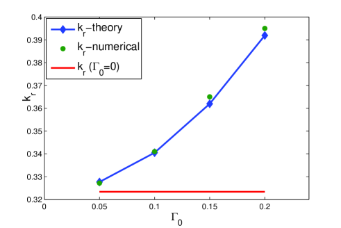
Figure 1: Nonlinear wavenumber $k_{r}$ v.s. pump amplitude $\Gamma_{0}$

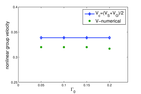
Figure 2: Nonlinear group velocity $v_{g}$ v.s. pump amplitude $\Gamma_{0}$

Figure 3: Nonlinear GAM frequency $\omega^{NL}$ v.s. pump amplitude $\Gamma_{0}$

The nonlinear frequency of GAM is given in Fig. 3, where the dots are numerical results and the diamonds represents $\omega_{NL}$ from equation (11). Note that, for the parameters we use here, $\omega_{0}=0.105$, and the nonlinear frequency from numerical solution increases with pump DW amplitude as predicted by our theory.

IV Conclusions and Discussions

In conclusion, equations describing the spatialtemporal evolution of parametrically excited GAM initial pulse are studied both analytically and numerically. It is found that the parametrically excited GAM propagates at a nonlinear group velocity, which is the mean of the linear group velocities of GAM and DW, and is much larger than that predicted by linear theory of kinetic GAM. The wavevector of the excited GAM has a quadratic dependence on the amplitude of the constant-amplitude pump DW. On the other hand, the nonlinear group velocity is independent of the pump DW amplitude; suggesting it as a good candidate for the comparison between experiments and analytical theory. Our nonlinear theory, further shows that there is a nonlinear upshift in the GAM frequency. Implications of the present theoretical findings to the HT-7 experimental observations are also important. Our results demonstrate that one must include nonlinear effects in order to properly analyze numerical simulations and/or experimental observations of GAM.

We note that, while the ambient turbulence in experiments consists of a whole spectrum of nonlinearly interacting DWs, we have, in the present analysis, considered the modification of the GAM dispersion relation due to a single-$n$ DW with finite amplitude. This can be justified, since DW interactions with ZS, e.g. GAMs, have two components: a coherent part due to the interaction with the self-generated ZS, and a random contribution due to interaction with ZS produced by other incoherent components of the fluctuation spectrum FZoncaNJP2015 . In both cases, the coupling coefficient is proportional to DW intensity and, therefore, we focus here on the coherent GAM-DW interaction FZoncaEPL2008 . Effects of system nonuniformities, which are shown to play important roles on the nonlinear interactions between GAM and DWs are also ignored here. This will limit the applications of our nonlinear theory. To properly interprete global numerical simulations and/or experimental results, more in-depth investigations taking into account system nonunifomities will be needed.

References

References

- (1) N. Winsor, J. L. Johnson, and J. M. Dawson, Physics of Fluids 11, 2448 (1968).
- (2) F. Zonca and L. Chen, Europhys. Lett. 83, 35001 (2008).
- (3) A. Hasegawa, C. G. Maclennan, and Y. Kodama, Physics of Fluids 22, 2122 (1979).
- (4) M. N. Rosenbluth and F. L. Hinton, Phys. Rev. Lett. 80, 724 (1998).
- (5) W. Horton, Rev. Mod. Phys. 71, 735 (1999).
- (6) L. Chen and F. Zonca, Phys. Rev. Lett. 109, 145002 (2012).
- (7) Z. Qiu, L. Chen, and F. Zonca, EPL (Europhysics Letters) 101, 35001 (2013).
- (8) Z. Qiu, L. Chen, and F. Zonca, Physics of Plasmas (1994-present) 21, 022304 (2014).
- (9) Z. Lin, T. S. Hahm, W. W. Lee, W. M. Tang, and R. B. White, Science 281, 1835 (1998).
- (10) P. Liewer, Nuclear Fusion 25, 543 (1985).
- (11) Z. Feng, Z. Qiu, and Z. Sheng, Physics of Plasmas (1994-present) 20, 122309 (2013).
- (12) R. Sagdeev and A. Galeev., Nonlinear plasma theory (AW Benjamin Inc., 1969).
- (13) P. K. Kaw and J. M. Dawson, Physics of Fluids 12, 2586 (1969).
- (14) Z. Qiu, F. Zonca, and L. Chen, Plasma Science and Technology 13, 257 (2011).
- (15) R. Hager and K. Hallatschek, Physics of Plasmas 19, 082315 (pages 8) (2012).
- (16) L. Chen, F. Zonca and Z. Qiu, “Theoretical Studies of GAM Dynamics”, Presented at the joint Varenna-Lausanne International Workshop on “Theory of Fusion Plasmas”, Aug. 30 - Sep. 3 (2010), Varenna, Italy.
- (17) T. Ido, Y. Miura, K. Kamiya, Y. Hamada, K. Hoshino, A. Fujisawa, K. Itoh, S.-I. Itoh, A. Nishizawa, H. Ogawa, et al., Plasma Physics and Controlled Fusion 48, S41 (2006).
- (18) G. D. Conway, C. Troster, B. Scott, K. Hallatschek, and the ASDEX Upgrade Team, Plasma Physics and Controlled Fusion 50, 055009 (2008).
- (19) D. Kong, A. Liu, T. Lan, Z. Qiu, H. Zhao, H. Sheng, C. Yu, L. Chen, G. Xu, W. Zhang, et al., Nuclear Fusion 53, 113008 (2013).
- (20) Y. Hamada, T. Watari, A. Nishizawa, et. al., Plasma Physics and Controlled Fusion 51, 012001 (2009).
- (21) Z. Qiu, L. Chen, and F. Zonca, Plasma Physics and Controlled Fusion 51, 012001 (2009).
- (22) A. Boozer, Physics of Fluids 24, 1999 (1981).
- (23) L. Chen, Z. Lin, and R. White, Physics of Plasmas 7, 3129 (2000).
- (24) F. Romanelli and F. Zonca, Physics of Fluids B 5 (1993).
- (25) F. Zonca, L. Chen, S. Briguglio, G. Fogaccia, G. Vlad and X. Wang, New Journal of Physics 17, 013052, (2015).
- (26) M. N. Rosenbluth, Phys. Rev. Lett. 29, 565 (1972).
- (27) N. Chakrabarti, P. N. Guzdar, R. G. Kleva, V. Naulin, J. J. Rasmussen, and P. K. Kaw, Physics of Plasmas 15, 112310 (pages 5) (2008).
- (28) D. Kong, private communication, (2008).