AND
Quantization Design for Distributed Optimization
Abstract
We consider the problem of solving a distributed optimization problem using a distributed computing platform, where the communication in the network is limited: each node can only communicate with its neighbours and the channel has a limited data-rate. A common technique to address the latter limitation is to apply quantization to the exchanged information. We propose two distributed optimization algorithms with an iteratively refining quantization design based on the inexact proximal gradient method and its accelerated variant. We show that if the parameters of the quantizers, i.e. the number of bits and the initial quantization intervals, satisfy certain conditions, then the quantization error is bounded by a linearly decreasing function and the convergence of the distributed algorithms is guaranteed. Furthermore, we prove that after imposing the quantization scheme, the distributed algorithms still exhibit a linear convergence rate, and show complexity upper-bounds on the number of iterations to achieve a given accuracy. Finally, we demonstrate the performance of the proposed algorithms and the theoretical findings for solving a distributed optimal control problem.
I Introduction
Distributed optimization methods for networked systems that have many coupled sub-systems and must act based on local information, are critical in many engineering problems, e.g. resource allocation, distributed estimation and distributed control problems. The algorithms are required to solve a global optimization problem in a distributed fashion subject to communication constraints.
Inexact distributed optimization methods are attracting increasing attention, since these techniques have the potential to deal with errors, for instance caused by inexact solution of local problems as well as unreliable or limited communication, e.g., transmission failures and quantization errors. Previous work has aimed at addressing the questions of how such errors affect the algorithm and under what conditions the convergence of the distributed algorithms can be guaranteed. In [7], the authors propose an inexact decomposition algorithm for solving distributed optimization problems by employing smoothing techniques and an excessive gap condition. In our previous work [12], we have proposed an inexact splitting method, named the inexact fast alternating minimization algorithm, and applied it to distributed optimization problems, where local computation errors as well as errors resulting from limited communication are allowed, and convergence conditions on the errors are derived based on a complexity upper-bound. Some other related references for inexact optimization algorithms include [6], [10] and [14]. In [14], an inexact proximal-gradient method, as well as its accelerated version, are introduced. The proximal gradient method, also known as the iterative shrinkage-thresholding algorithm (ISTA) [1], has two main steps: the first one is to compute the gradient of the smooth objective and the second one is to solve the proximal minimization. The conceptual idea of the inexact proximal-gradient method is to allow errors in these two steps, i.e. an error in the calculation of the gradient and an error in the proximal minimization. The results in [14] show convergence properties of the inexact proximal-gradient method and provide conditions on the errors, under which convergence of the algorithm can be guaranteed.
We consider a distributed optimization problem, where each sub-problem has a local cost function that involves both local and neighbouring variables, and local constraints on local variables. The problem is solved in a distributed manner with only local communication, i.e. between neighbouring sub-systems. In addition, the communication bandwidth between neighbouring sub-systems is limited. In order to meet the limited communication data-rate, the information exchanged between the neighbouring sub-systems needs to be quantized. The quantization process results in inexact iterations throughout the distributed optimization algorithm, which effects its convergence. Related work includes [3], [9], [15] and [11], which study the effects of quantization on the performance of averaging or distributed optimization algorithms.
We propose two distributed optimization algorithms with progressive quantization design building on the work in [14] and [15]. The main idea behind the proposed methods is to apply the inexact gradient method to the distributed optimization problem and to employ the error conditions, which guarantee convergence to the global optimum, to design a progressive quantizer. Motivated by the linear convergence upper-bound of the optimization algorithm, the range of the quantizer is set to reduce linearly at a rate smaller than one and larger than the rate of the algorithm, in order to refine the information exchanged in the network with each iteration and achieve overall converge to the global optimum. The proposed quantization method is computationally cheap and consistent throughout the iterations as every node implements the same quantization procedure.
This work extends the initial ideas presented in [13] for designing a quantization scheme for unconstrained distributed optimization. In particular, the paper makes the following main extensions and contributions:
-
•
Constrained optimization problems: We consider distributed optimization problems with convex local constraints. To handle the constraints, two projection steps are required. One is applied before the information exchange, and the other after. The reason to have a second projection is that after the information exchange, the quantized value received by each agent can be an infeasible solution subject to the local constraints. The second projection step therefore guarantees that at each iteration every agent has a feasible solution for the computation of the gradient. We present conditions on the number of bits and the initial quantization intervals, which guarantee convergence of the algorithms. We show that after imposing the quantization scheme including the two projections, the algorithms preserve the linear convergence rate, and furthermore derive complexity upper-bounds on the number of iterations to achieve a given accuracy. In addition, we provide a discussion about how the minimum number of bits and the corresponding minimum initial quantization intervals can be obtained.
-
•
Accelerated algorithm: We propose an accelerated variant of the distributed optimization algorithm with quantization refinement based on the inexact accelerated proximal-gradient method. With the acceleration step, the algorithm preserves the linear convergence rate, but the constant of the rate will be improved.
-
•
Distributed optimal control example: We demonstrate the performance of the proposed method and the theoretical results for solving an distributed optimal control example.
II Preliminaries
II-A Notation
Let be a vector. and denote the and infinity norms of , respectively. Note that . Let be a subset of . The projection of any point onto the set is denoted by . Let be a strongly convex function; denotes the convexity modulus for any , where denotes the set of sub-gradients of the function at a given point. denotes a Lipschitz constant of the function , i.e. , . The proximity operator is defined as
| (1) |
We refer to [2] and [8] for details on the definitions and properties above. The proximity operator with an extra subscript , i.e. , means that a maximum computation error is allowed in the proximal objective function:
| (2) |
II-B Inexact Proximal-Gradient Method
In this section, we will introduce the inexact proximal-gradient method (inexact PGM) proposed in [14]. Inexact PGM is presented in Algorithm 1. It addresses optimization problems of the form given in Problem II.1 and requires Assumption II.2 for convergence with a linear rate.
Problem II.1
Assumption II.2
-
•
is a strongly convex function with a convexity modulus and Lipschitz continuous gradient with Lipschitz constant .
-
•
is a lower semi-continuous convex function, not necessarily smooth.
Inexact PGM in Algorithm 1 allows two kinds of errors: represents the error in the gradient calculations of , and represents the error in the computation of the proximal minimization in (2) at every iteration . The following proposition states the convergence property of inexact PGM.
Proposition II.3 (Proposition 3 in [14])
As discussed in [14], the upper-bound in Proposition II.3 allows one to derive sufficient conditions on the error sequences and for convergence of the algorithm to the optimal solution , where :
-
•
If the series and decrease at a linear rate with the constant , then converges at a linear rate with the constant .
-
•
If the series and decrease at a linear rate with the constant , then converges at the same rate with the constant .
-
•
If the series and decrease at a linear rate with the constant , then converges at a rate of .
II-C Inexact Accelerated Proximal-Gradient Method
In this section, we introduce an accelerated variant of inexact PGM, named the inexact accelerated proximal-gradient method (inexact APGM) proposed in [14]. Compared to inexact PGM, it addresses the same problem class in Problem II.1 and requires the same assumption in Assumption II.2 for linear convergence, but involves one extra linear update in Algorithm 2, which improves the constant of the linear convergence rate from to .
Proposition 4 of [14] presents a complexity upper-bound on the sequence , where the sequence is generated by inexact APGM. The following proposition extends this result and states a complexity upper-bound on .
Proposition II.5
The proof of Proposition II.5 will be given in the appendix in Section V-A. The upper-bound in Proposition II.5 provides similar sufficient conditions on the error sequences and for the convergence of Algorithm 2, which are obtained by replacing in the sufficient conditions for Algorithm 1 in Section II-B with .
II-D Uniform quantizer
Let be a real number. A uniform quantizer with a quantization step-size and the mid-value can be expressed as
| (5) |
where is the sign function. The parameter is equal to , where represents the size of the quantization interval and is the number of bits sent by the quantizer. In this paper, we assume that is a fixed number, which means that the quantization interval is set to be . The quantization error is upper-bounded by
| (6) |
For the case that the input of the quantizer and the mid-value are not real numbers, but vectors with the same dimension , the quantizer is composed of independent scalar quantizers in (5) with the same quantization interval and corresponding mid-value. In this paper, we design a uniform quantizer denoted as with changing quantization interval and mid-value at every iteration of the optimization algorithm.
III Distributed optimization with limited communication
In this section, we propose two distributed optimization algorithms with progressive quantization design based on the inexact PGM algorithm and its accelerated variant. The main challenge is that the communication in the distributed optimization algorithms is limited and the information exchanged in the network needs to be quantized. We propose a progressive quantizer with changing parameters, which satisfies the communication limitations, while ensuring that the errors induced by quantization satisfy the conditions for convergence.
III-A Distributed optimization problem
In this paper, we consider a distributed optimization problem on a network of sub-systems (nodes). The sub-systems communicate according to a fixed undirected graph . The vertex set represents the sub-systems and the edge set specifies pairs of sub-systems that can communicate. If , we say that sub-systems and are neighbours, and we denote by the set of the neighbours of sub-system . Note that includes . We denote as the degree of the graph . The optimization variable of sub-system and the global variable are denoted by and , respectively. For each sub-system , the local variable has a convex local constraint . The constraint on the global variable is denoted by . The dimension of the local variable is denoted by and the maximum dimension of the local variables is denoted by , i.e. . The concatenation of the variable of sub-system and the variables of its neighbours is denoted by , and the corresponding constraint on is denoted by . With the selection matrices and , they can be represented as and , , which implies the relation between the local variable and the global variable , i.e. , . Note that and are selection matrices, and therefore . We solve a distributed optimization problem of the formulation in Problem III.1:
Problem III.1
Assumption III.2
We assume that the global cost function is strongly convex with a convexity modulus and Lipschitz continuous gradient with Lipschitz constant , i.e. for any and .
Assumption III.3
The local constraint is a convex set, for .
Assumption III.4
We assume that every local cost function has Lipschitz continuous gradient with Lipschitz constant , and denote as the maximum Lipschitz constant of the local functions, i.e. .
III-B Qualitative description of the algorithm
In this section, we provide a qualitative description of the distributed optimization algorithm with quantization refinement to introduce the main idea of the approach. We apply the inexact PGM algorithm to the distributed optimization problem in Problem III.1, where the two objectives in Problem II.1 are chosen as and , where denotes the indicator function on the set . The parameter is equal to
| (7) |
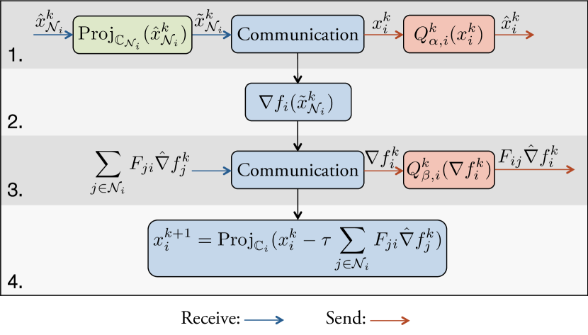
The communication in the network is limited: each sub-system in the network can only communicate with its neighbours, and at each iteration, only a fixed number of bits can be transmitted. Only considering the first limitation, the distributed optimization algorithm resulting from applying the inexact PGM algorithm to Problem III.1 is represented by the blue boxes in Fig. 1. At iteration , sub-system carries out four main steps:
-
1.
Send the local variable to its neighbours;
-
2.
Compute the local gradient;
-
3.
Send the local gradient to its neighbours;
-
4.
Update the local variable and compute the projection of the updated local variable on the local constraint.
To handle the second limitation, we design two uniform quantizers (the salmon-pink boxes) for the two communication steps for each sub-system and using a varying quantization interval and mid-value to refine the exchanged information at each iteration. Motivated by the second sufficient condition on the error sequences and for the convergence of the inexact PGM algorithm discussed in Section II-B (if the sequences and decrease at a linear rate with the constant , then converges with the same rate), the quantization intervals are set to be a linearly decreasing function and , with and two constants and as the initial intervals. We know that if for every , the values and fall inside the quantization intervals, the quantization errors converge at the same linear rate with the constant . In Section III-C, we will show that by properly choosing the number of bits and the initial intervals and , it can be guaranteed that and fall inside the quantization intervals at every iteration and the quantization errors decrease linearly.
We add an extra re-projection step (green box) into the algorithm, because the quantized value can be an infeasible solution with respect to the constraints . The re-projection step guarantees that at each iteration the gradient is computed based on a feasible solution. Using the convexity of the constraints, we can show that the error caused by the re-projected point is upper-bounded by the quantization error. To summarize, all the errors induced by the limited communication in the distributed algorithm are upper bounded by a linearly decreasing function with the constant , which implies that the distributed algorithm with quantization converges to the global optimum and the linear convergence rate is preserved. These results will be shown in detail in Section III-C.
III-C Distributed algorithm with quantization refinement
In this section, we propose a distributed algorithm with a progressive quantization design in Algorithm 3. For every sub-system , there are two uniform quantizers and using the formulation introduced in Section II-D with a fixed number of bits , changing quantization intervals and and changing mid-values and for transmitting , and at every iteration . At iteration , the quantization intervals are set to be and , and the mid-values are set to be the previous quantized values and . The two parameters and denote the initial quantization intervals.
In this paper, is used to denote a quantized value, e.g. and is used to denote a re-projected value, e.g. . The quantization errors are denoted by and .
Remark III.5
We want to highlight Step 4 in Algorithm 3, because it is the key step that allows us to extend the algorithm in [13] for solving an unconstrained distributed optimization problem to constrained problems. The re-projection step ensures that the point used to compute the gradient at each iteration is a feasible solution subject to the constraints , which is a necessary condition for the convergence of the algorithm.
In the following, we present four lemmas that link Algorithm 3 to the inexact PGM and prove that Algorithm 3 converges linearly to the global optimum despite the quantization errors. Lemma III.6 states that due to the fact that the constraints are convex, the error between the re-projected point and the original point is upper-bounded by the quantization error. Lemma III.7 shows that the inexactness resulting from quantization in Algorithm 3 can be considered as the error in the gradient calculation and the error in the computation of the proximal minimization in Algorithm 1. Lemma III.9 states that if at each iteration the values and fall inside the quantization intervals, then the errors caused by quantization decrease linearly and the algorithm converges to the global optimum at the same rate. Lemma III.13 gives conditions on the number of bits and the initial quantization intervals, which guarantee that and fall inside the quantization intervals for each iteration. Once we prove the three lemmas, we are ready to present the main result in Theorem III.14.
Lemma III.6
Let be a convex subset of and . For any point , the following holds:
| (8) |
Lemma III.7
Remark III.8
Lemma III.7 shows that the errors and are upper-bounded by functions of the quantization errors and . We want to emphasize that the quantization errors and are not necessarily bounded by a linear function with the rate . They are bounded only if the values and fall inside the quantization intervals that are decreasing at a linear rate. Otherwise, the quantization errors and can be arbitrarily large.
From the discussion in Section II-B, we know that if and decrease linearly at a rate larger than , then converges linearly at the same rate as . Lemma III.9 provides the first step towards achieving this goal. It shows that if the values of and always fall inside the quantization interval, then the computational error of the gradient and the computational error of the proximal operator as well as decrease linearly with the constant .
Lemma III.9
For any parameter satisfying and a , if for all the values of and generated by Algorithm 3 fall inside of the quantization intervals of and , i.e. and , then the error sequences and satisfy
| (11) |
where and , and satisfies
| (12) |
The proof of Lemma III.9 will be provided in the appendix in Section V-C. From Lemma III.9, we know that the last missing piece is to show that the values and fall inside the quantization interval at every iteration . The following assumption presents conditions on the number of bits and the initial quantization intervals and , which guarantee that for each iteration and in Algorithm 3 fall inside the changing quantization intervals and the quantization errors decrease linearly with the constant , which further implies that the Algorithm 3 converges to the global optimum linearly with the same rate .
Assumption III.10
Consider the quantizers and in Algorithm 3. We assume that the parameters of the quantizers, i.e. the number of bits and the initial quantization intervals and satisfy
| (13) |
| (14) |
with
Remark III.11
The parameters of the quantizers , and are all positive constants. Assumption III.10 can always be satisfied by increasing , and .
Remark III.12
For a fixed , inequalities (13) and (14) represent two polyhedral constraints on and . Therefore, the minimal and can be computed by solving a simple LP problem, i.e. minimizing subject to , , and inequalities (13) and (14). Since the minimal is actually the minimal one guaranteeing that the LP problem has a feasible solution, the minimal can be found by testing feasibility of the LP problem.
Lemma III.13
The proof of Lemma III.13 will be provided in the appendix in Section V-D. After showing Lemma III.7, Lemma III.9 and Lemma III.13, we are ready to present the main theorem.
Theorem III.14
Proof:
Since Assumption III.2, III.4 and III.10 hold, Lemma III.13 states that for each iteration the values and in Algorithm 3 fall inside of the quantization intervals of and . Then from Lemma III.9, we know that the error sequences and satisfy and , and by Lemma III.7 the sequence generated by Algorithm 3 satisfies inequality (15). ∎
Recalling the complexity bound in Proposition II.3, we know that for the case without errors the algorithm converges linearly with the constant . After imposing quantization on the algorithm, it still converges to the global optimum linearly but with a larger constant . We conclude that with the proposed quantization design, the linear convergence of the algorithm is preserved, but the constant of the convergence rate has to be enlarged in order to compensate for the deficiencies from limited communication.
III-D Accelerated distributed algorithm with quantization refinement
In this section, we propose an accelerated variant of the distributed algorithm with quantization refinement in Algorithm 4 based on the inexact accelerated proximal gradient method in Algorithm 2. Compared to Algorithm 3, Algorithm 4 has an extra accelerating Step 5 , and at each iteration the gradient is computed based on . The accelerating step improves the constant of the linear convergence rate of the algorithms from to , and changes the condition on the quantization parameter to .
Lemma III.15
Proof:
The proof follows the same flow of the proof of Lemma III.7. The only difference is that at each iteration the gradient is computed based on , which is a linear combination of and . Hence, the upper-bound on the computational error of the gradient is a function of the linear combination of , and . ∎
Lemma III.16
For any parameter satisfying and a , if for all the values of and generated by Algorithm 4 fall inside of the quantization intervals of and , i.e. and , then the sequences and satisfy
| (18) |
where and , and satisfies
| (19) |
Proof:
Assumption III.17
We assume that the number of bits and the initial quantization intervals and satisfy
| (20) |
| (21) |
with
Lemma III.18
Theorem III.19
IV Numerical Example
This section illustrates the theoretical findings of the paper and demonstrates the performance of Algorithm 3 and Algorithm 4 for solving a distributed quadratic programming (QP) problem originating from the problem of regulating constrained distributed linear systems by model predictive control (MPC) in the form of Problem IV.1. For more information about distributed MPC, see e.g. [5], [4] and [12].
Problem IV.1
and denote the number of subsystems and the horizon of the MPC problem, respectively. The state and input sequences along the horizon of subsystem are denoted by and . The discrete-time linear dynamics of subsystem are given by , where and are the dynamic matrices. The initial state is denoted by . The control inputs of subsystem are subject to local convex constraints . and are strictly convex cost functions. From Problem IV.1, we can see that subsystem is coupled with its neighbours in the linear dynamics.
We randomly generate a distributed MPC problem in the form of Problem IV.1. We first randomly generate a connected network with sub-systems. Each sub-system has states and inputs. The dynamical matrices and are randomly generated, i.e. generally dense, and the local systems are controllable and unstable. The input constraint for sub-system is set to , where denotes the all-ones vector with the same dimension as . The horizon of the MPC problem is set to . The local cost functions are chosen as quadratic functions and , where , and are identity matrices. The initial states are chosen, such that more than of the optimization variables are at the constraints at optimality.
Problem IV.2
By eliminating all state variables distributed MPC problems of this class can be reformulated as a distributed QP of the form in Problem IV.2 with the local variables and the concatenations of the variables of subsystem and its neighbours . Matrix is dense and positive definite, and vector is dense. The constraint is a polytopic set.
Table I shows the parameters chosen in Algorithm 3 and Algorithm 4, including the constants of the convergence rate of the algorithms, i.e. and , the decrease rates of the quantization intervals satisfying for Algorithm 3 and for Algorithm 4 and the minimum number of bits required for convergence .
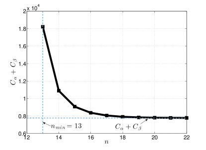
Fig. 2 shows the relationship between the number of bits and the minimum initial quantization intervals and , which satisfy Assumption III.10 for Problem IV.2. We see that the minimum number of bits required for convergence is equal to , and as the number of bits increases, the required minimum and decrease.
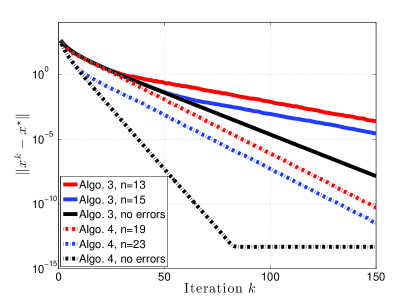
Fig. 3 shows the performance of Algorithm 3 and Algorithm 4 for solving the distributed QP problem in Problem IV.2 originating from the distributed MPC problem. For Algorithm 3, is set to and , respectively, and the initial quantization intervals and are set to corresponding minimum values satisfying Assumption III.10. For Algorithm 4, is set to and , and and to corresponding minimum values satisfying Assumption III.17. In Fig. 3 we can observe that the proposed distributed algorithms with quantization converges to the global optimum linearly and the performance is improved when the number of bits is increased. Due to the acceleration step, Algorithm 4 converges faster than Algorithm 3. However, Algorithm 4 requires a larger number of bits to guarantee the convergence.
| Parameters | Algorithm 3 | Algorithm 4 |
|---|---|---|
| Constant of rate | ||
V Appendix
V-A Proof of Proposition II.5
V-B Proof of Lemma III.7
V-C Proof of Lemma III.9
Proof:
From the property of the uniform quantizer, we know that if and fall inside of the quantization intervals of and , then the quantization errors and are upper-bounded by
where and denotes the degree of the graph of the distributed optimization problem. From Lemma III.7, we have
and
Since the quantization intervals are set to and , it implies that
and
with and , where . Since , Lemma III.7 and Proposition II.3 imply that for
Since , by using the property of geometric series, we get that the expression above is equal to
Hence, inequality (12) is proven. ∎
V-D Proof of Lemma III.13
Proof:
We will prove Lemma III.13 by induction.
-
•
Base case: When , since and are positive numbers and and are initialized to zero, it holds that and .
-
•
Induction step: Let be given and suppose that and for . We will prove that
(23) and
(24) for . We first show (23). From Algorithm 3, we know
Since and are selection matrices, then . The term above is upper-bounded by
By the assumption of the induction, we know and for . Then, using Lemma III.9, we obtain that the term above is upper-bounded by
By substituting and and using the parameters defined in Assumption III.10, it follows that the expression above is equal to
By inequality (13) in Assumption III.10, the term above is bounded by . Thus, inequality (23) holds. In the following, we prove that inequality (24) is true.
Since , and , Lemma III.6 implies and . Hence, the term above is upper-bounded by
Again by the assumption of the induction, we know and for . Then, Lemma III.9 implies that the term above is upper-bounded by
By substituting and and using the parameters defined in Assumption III.10, it follows that the expression above is equal to
By inequality (14) in Assumption III.10, the term above is bounded by . Thus, inequality (24) holds.
We conclude that by the principle of induction, the values of and in Algorithm 3 fall inside of the quantization intervals of and , i.e. and for all . ∎
V-E Proof of Lemma III.18
Proof:
The proof is similar to the proof of Lemma III.13. The difference is that at each iteration the gradient is computed based on , which is a linear combination of and . We therefore only show a brief proof for the second step, i.e. the inequality for any by induction.
-
•
Base case: When , since is positive a number, and are initialized to zero and , it holds that .
-
•
Induction step: Let be given and suppose that and for . We will prove
(25) From the algorithm, we know
By substituting , and , and using the fact that and , the expression above is upper-bounded by
By the assumption of the induction and Lemma III.16, we obtain that the above is upper-bounded by
By substituting and and using the parameters defined in Assumption III.17, the expression becomes
By inequality (21) in Assumption III.17, the term above is bounded by . Thus, the inequality holds. The proof of the induction step is complete.
By the principle of induction, we conclude that the inequality holds for any . ∎
References
- [1] A. Beck and M. Teboulle. A fast iterative shrinkage thresholding algorithm for linear inverse problems. SIAM Journal on Imaging Sciences, pages 183–202, 2009.
- [2] D. P. Bertsekas, A. Nedic, and A. E. Ozdaglar. Convex analysis and optimization. Athena Scientific Belmont, 2003.
- [3] R. Carli, F. Fagnani, P. Frasca, T. Taylor, and R. Zampieri. Average consensus on networks with transmission noise or quantization. In European Control Conference, pages 1852–1857, 2007.
- [4] C. Conte, T. Summers, M.N. Zeilinger, M. Morari, and C.N. Jones. Computational aspects of distributed optimization in model predictive control. In 51th IEEE Conference on Decision and Control, pages 6819–6824, 2012.
- [5] C. Conte, N. R. Voellmy, M. N. Zeilinger, M. Morari, and C. N. Jones. Distributed synthesis and control of constrained linear systems. In American Control Conference, pages 6017–6022, 2012.
- [6] O. Devolder, F. Glineur, and Y. Nesterov. First-order methods of smooth convex optimization with inexact oracle. Mathematical Programming, pages 1–39, 2013.
- [7] Q. T. Dinh, I. Necoara, and M. Diehl. Fast inexact decomposition algorithms for large-scale separable convex optimization. arXiv preprint arXiv:1212,4275, 2012.
- [8] R. A. Horn and C. R. Johnson. Matrix Analysis. Cambridge University Press, 1990.
- [9] A. Kashyap, T. Basar, and R. Srikant. Quantized consensus. Automatica, 43:1192–1203, 2007.
- [10] V. Nedelcu, I. Necoara, and I. Dumitrache. Complexity of an inexact augmented lagrangian method: Application to constrained MPC. In 19th World Congress of the International Federation of Automatic Control, pages 2927–2932, 2014.
- [11] A. Nedic, A. Olshevsky, A. Ozdaglar, and J.N. Tsitsiklis. Distributed subgradient methods and quantization effects. In 47th IEEE Conference on Decision and Control, pages 4177–4184, 2008.
- [12] Y. Pu, M.N. Zeilinger, and C. N. Jones. Inexact fast alternating minimization algorithm for distributed model predictive control. In 53th IEEE Conference on Decision and Control, pages 5915–5921, 2014.
- [13] Y. Pu, M.N. Zeilinger, and C. N. Jones. Quantization design for unconstrained distributed optimization. In American Control Conference, 2015.
- [14] M. Schmidt, N. L. Roux, and F. Bach. Convergence rates of inexact proximal-gradient methods for convex optimization. In 25th Annual Conference on Neural Information Processing Systems, pages 6819–6824, 2011.
- [15] D. Thanou, E. Kokiopoulou, Y. Pu, and P. Frossard. Distributed average consensus with quantization refinement. IEEE Transactions on Signal Processing, 61:194–205, 2013.