Entropy power inequalities for qudits

Abstract

Shannon’s entropy power inequality (EPI) can be viewed as a statement of concavity of an entropic function of a continuous random variable under a scaled addition rule:

$$f(\sqrt{a}\,X+\sqrt{1-a}\,Y)\geq af(X)+(1-a)f(Y)\quad\forall\,a\in[0,1].$$

Here, $X$ and $Y$ are continuous random variables and the function $f$ is either the differential entropy or the entropy power. König and Smith [IEEE Trans. Inf. Theory. 60(3):1536–1548, 2014] and De Palma, Mari, and Giovannetti [Nature Photon. 8(12):958–964, 2014] obtained quantum analogues of these inequalities for continuous-variable quantum systems, where $X$ and $Y$ are replaced by bosonic fields and the addition rule is the action of a beamsplitter with transmissivity $a$ on those fields. In this paper, we similarly establish a class of EPI analogues for $d$-level quantum systems (i.e. qudits). The underlying addition rule for which these inequalities hold is given by a quantum channel that depends on the parameter $a\in[0,1]$ and acts like a finite-dimensional analogue of a beamsplitter with transmissivity $a$, converting a two-qudit product state into a single qudit state. We refer to this channel as a partial swap channel because of the particular way its output interpolates between the states of the two qudits in the input as $a$ is changed from zero to one. We obtain analogues of Shannon’s EPI, not only for the von Neumann entropy and the entropy power for the output of such channels, but for a much larger class of functions as well. This class includes the Rényi entropies and the subentropy. We also prove a qudit analogue of the entropy photon number inequality (EPnI). Finally, for the subclass of partial swap channels for which one of the qudit states in the input is fixed, our EPIs and EPnI yield lower bounds on the minimum output entropy and upper bounds on the Holevo capacity.

1 Introduction

Inequalities between entropic quantities play a fundamental role in information theory and have been employed effectively in finding bounds on optimal rates of various information-processing tasks. Shannon’s entropy power inequality (EPI) [Sha48] is one such inequality and it has proved to be of relevance in studying problems not only in information theory, but also in probability theory and mathematical physics [Sta59]. It has been used, for example, in finding upper bounds on the capacities of certain noisy channels (e.g. the Gaussian broadcast channel [Ber74]) and in proving convergence in relative entropy for the Central Limit Theorem [Bar86].

Classical EPIs

For an arbitrary random variable $X$ on $\mathbb{R}^{d}$ with probability density function (p.d.f.) $f_{X}$, the entropy power of $X$ is the quantity

$$v(X):=\frac{e^{2H(X)/d}}{2\pi e},$$ (1.1)

where $H(X)$ is the differential entropy of $X$,

$$H(X):=-\int_{\mathbb{R}^{d}}f_{X}(x)\log f_{X}(x)dx$$ (1.2)

(throughout the paper we use $\log$ to represent the natural logarithm). The name “entropy power” is derived from the following fact: if $X$ is a Gaussian random variable on $\mathbb{R}$ with zero mean and variance $\sigma^{2}$, then $H(X)=(1/2)\log(2\pi e\sigma^{2})$; hence $v(X)$ is equal to its variance, which is commonly referred to as its power. Note that the entropy power of a random variable $X$ is equal to the variance of a Gaussian random variable which has the same differential entropy as $X$. For $X$ on $\mathbb{R}^{d}$, we shall henceforth omit the factor $1/2\pi e$ and refer to $e^{2H(X)/d}$ as the entropy power, as in [KS14].

The entropy power satisfies the following scaling property: $v(\sqrt{\alpha}X)=\alpha v(X)$. This follows from the scaling property of p.d.f.s: if $f_{\alpha X}$ denotes the p.d.f. of a random variable $\alpha X$ on $\mathbb{R}^{d}$, where $\alpha>0$, then $f_{\alpha X}(x)=\alpha^{-d}f_{X}(x/\alpha)$, $x\in\mathbb{R}^{d}$, which in turn implies that $H(\alpha X)=H(X)+d\log\alpha$. This shows why the factor $1/d$ in the definition of $v(X)$ has to be there for $X$ on $\mathbb{R}^{d}$.

Shannon’s EPI [Sha48] provides a lower bound on the entropy power of a sum of two independent random variables $X$ and $Y$ on $\mathbb{R}^{d}$ in terms of the sums of the entropy powers of the individual random variables:

$$v(X+Y)\geq v(X)+v(Y),$$ (1.3)

or equivalently,

$$e^{2H\lparen X+Y\rparen/d}\geq e^{2H(X)/d}+e^{2H(Y)/d}.$$ (1.4)

Here, $H(X+Y)$ is the differential entropy of the p.d.f. of the sum $Z:=X+Y$, which is given by the convolution

$$f_{X+Y}(x)=(f_{X}\ast f_{Y})(x):=\int_{\mathbb{R}^{d}}f_{X}(x^{\prime})f_{Y}(x-x^{\prime})dx^{\prime},\qquad\forall\,x\in\mathbb{R}^{d}.$$ (1.5)

The inequality eq. 1.3 was proposed by Shannon in [Sha48] as a means to bound the capacity of a non-Gaussian additive noise channel, that is, a channel with input $X$ and output $X+Y$, with $Y$ being an independent (non-Gaussian) random variable modeling the noise which is added to the input. Later, Lieb [Lie78] and Dembo, Cover, and Thomas [DCT91] (see also [VG06]) showed that the EPI (1.4) can be equivalently expressed as the following inequality between differential entropies:

$$H\big{\lparen}\sqrt{a}\,X+\sqrt{1-a}\,Y\big{\rparen}\geq aH(X)+(1-a)H(Y),\qquad\forall\,a\in[0,1].$$ (1.6)

The above inequality was proved by employing the Rényi entropy [Rén61] and using properties of $p$-norms on convolutions given by a sharp form of Young’s inequality [Bec75].

The form of the EPI in eq. 1.6 motivates the definition of an operation (which following [KS13b, KS14] we denote as $\boxplus_{a}$) on the space of random variables, given by the following scaled addition rule:

$$X\boxplus_{a}Y:=\sqrt{a}\,X+\sqrt{1-a}\,Y,\qquad\forall\,a\in[0,1].$$ (1.7)

The random variable $X\boxplus_{a}Y$ can be interpreted as an interpolation between $X$ and $Y$ as $a$ is decreased from $1$ to $0$. With this notation, the inequality (1.6) can be written as

$$H\lparen X\boxplus_{a}Y\rparen\geq aH(X)+(1-a)H(Y),\qquad\forall\,a\in[0,1].$$ (1.8)

Using the scaling property of the entropy power, the EPI (1.4) can be expressed as follows:

$$e^{2H\lparen X\boxplus_{a}Y\rparen/d}\geq ae^{2H(X)/d}+(1-a)e^{2H(Y)/d},\qquad\forall\,a\in[0,1].$$ (1.9)

Shannon’s EPI (1.4) (and hence also (1.8) and (1.9)) was first proved rigorously by Stam [Sta59] and by Blachman [Bla65], by employing de Bruijn’s identity, which couples Fisher information with differential entropy. Since then various different proofs and generalizations of the EPI have been proposed (see e.g. [VG06, Rio11, SS15] and references therein).

It is natural to conjecture that an analogue of Shannon’s EPI also holds for discrete random variables e.g. on non-negative integers. This conjecture was first proved by [HV03] for the case of binomial random variables. They proved that if $X_{n}\sim\mathrm{Bin}(n,p)$, then for $p=1/2$ (see also [SDM11]):

$$e^{2H\lparen X_{n}+X_{m}\rparen}\geq e^{2H(X_{n})}+e^{2H(X_{m})},\qquad\forall\,m,n\geq 1.$$ (1.10)

Further, Johnson and Yu [JY10] established a form of the EPI which is valid for ultra log-concave discrete random variables (see Definition 2.2 of [JY10]), whereby the scaling operation of a continuous random variable was suitably replaced by the so-called thinning operation introduced by Rényi [Rén56], which is considered to be an analogue of scaling for discrete random variables.

Quantum analogues of EPIs

The discovery of an analogue of the EPI in the quantum setting by König and Smith [KS14] marked a significant advance in quantum information theory. They proposed an EPI which holds for continuous-variable quantum systems that arise, for example, in quantum optics. In this case, the random variables $X$, $Y$ of the classical EPIs (eq. 1.8 and eq. 1.9) are replaced by quantum fields, bosonic modes of electromagnetic radiation, described by quantum states $\rho_{X}$, $\rho_{Y}$, which act on a separable, infinite-dimensional Hilbert space $\mathcal{H}$. The differential entropy is accordingly replaced by the von Neumann entropy $H(\rho):=-\operatorname{Tr}(\rho\log\rho)$.

A prerequisite for any quantum analogue of the EPI is the formulation of a suitable analogue of the addition rule (1.7) which can be applied to pairs of quantum states. Since the quantum-mechanical analogue of additive noise can be modelled by the mixing of two beams of light at a beamsplitter, König and Smith considered the parameter $a$ in eq. 1.7 to be the beamsplitter’s transmissivity. The classical addition rule eq. 1.7 is thereby replaced by an analogous quantum field addition rule for the field operators. In particular, if the two input signals are $m$-mode bosonic fields, with annihilation operators $\hat{a}_{1},\dotsc,\hat{a}_{m}$ and $\hat{b}_{1},\dotsc,\hat{b}_{m}$ respectively, then the output is an $m$-mode bosonic field with annihilation operators $\hat{c}_{1},\dotsc,\hat{c}_{m}$, where

$$\hat{c}_{i}:=\sqrt{a}\,\hat{a}_{i}+\sqrt{1-a}\,\hat{b}_{i}.$$ (1.11)

In a state space description, the input signals are described by quantum states $\rho_{X}$, $\rho_{Y}$ on $\mathcal{H}$. This yields an equivalent quantum state addition rule, where the beamsplitter converts the incoming state $\rho_{X}\otimes\rho_{Y}$ to a state $\rho_{X}\boxplus_{a}\rho_{Y}$ given by

$$(\rho_{X},\rho_{Y})\mapsto\rho_{X}\boxplus_{a}\rho_{Y}:=\mathcal{E}_{a}(\rho_{X}\otimes\rho_{Y}).$$ (1.12)

Here, $\mathcal{E}_{a}$ is a linear, completely positive trace-preserving map defined through the relation

$$\mathcal{E}_{a}(\rho_{XY}):=\operatorname{Tr}_{Y}(U_{a}\rho_{XY}U_{a}^{\dagger}),$$ (1.13)

with the partial trace being taken over the second system, and $U_{a}$ is the unitary operator describing the action of the beamsplitter on the state space $\mathcal{H}$. Analogous to the classical case, the state $\rho_{X}\boxplus_{a}\rho_{Y}$ reduces to $\rho_{X}$ when $a=1$, and to $\rho_{Y}$ when $a=0$.

König and Smith [KS14] proved that the following quantum analogues of the EPIs (1.8) and (1.9) hold, under the quantum addition rule given by eq. 1.12:

$$H(\rho_{X}\boxplus_{a}\rho_{Y}) \geq aH(\rho_{X})+(1-a)H(\rho_{Y}),$$ (1.14)

$$e^{H(\rho_{X}\boxplus_{1/2}\rho_{Y})/m} \geq\frac{1}{2}e^{H(\rho_{X})/m}+\frac{1}{2}e^{H(\rho_{Y})/m},$$ (1.15)

where $m$ is the number of bosonic modes. The inequality (1.15) corresponds to a 50 : 50 beamsplitter (i.e., a beamsplitter with transmissivity $a=1/2$). Later, De Palma et al. [DMG14] proved that an analogous inequality also holds for any beamsplitter (i.e., for any $a\in[0,1]$) and is given by the following:

$$e^{H(\rho_{X}\boxplus_{a}\rho_{Y})/m}\geq ae^{H(\rho_{X})/m}+(1-a)e^{H(\rho_{Y})/m},\qquad\forall\,a\in[0,1].$$ (1.16)

Note that the EPI given by eq. 1.15 seems to differ from its classical counterpart (1.9) by a factor of $2$ in the exponent. However, one can argue that the dimension of the bosonic phase space is $d=2m$ (as there are 2 quadratures per mode). These EPIs have found applications for bounding classical capacity of bosonic channels [KS13b, KS13a].

The above inequalities do not reduce to the classical EPIs (1.8) and (1.9) for commuting states; in other words, they are not quantum generalizations of the Shannon’s original EPI in the usual sense, as they do not include the latter as a special case. This is because the addition rule acts at the field operator level and not at the state level. In fact, the dependence of the output state on the parameter $a$ is much more complicated than in the classical case.

Another inequality, related to the EPI (1.16), was conjectured by Guha et al. [GES08] and is known as the entropy photon number inequality (EPnI). The thermal state of a bosonic mode with annihilation operator $\hat{a}$ can be expressed as [GSE08]:

$$\rho_{T}=\sum_{i=0}^{\infty}\frac{N^{i}}{(N+1)^{i+1}}|i\rangle\langle i|,$$ (1.17)

where $N:=\operatorname{Tr}\lparen\rho_{T}\,\hat{a}^{\dagger}\hat{a}\rparen$ is the average photon number of the state $\rho_{T}$. Its von Neumann entropy can be evaluated as $H(\rho_{T})=g(N)$ where $g(x):=(1+x)\log(1+x)-x\log x$. Inverting this, the photon number of $\rho_{T}$ is then $N=g^{-1}\lparen H(\rho_{T})\rparen$. Correspondingly, the photon number of an $m$-mode bosonic state $\rho$ is defined as $N(\rho):=g^{-1}\lparen H(\rho)/m\rparen$. Guha et al. [GES08] conjectured that

$$N(\rho_{X}\boxplus_{a}\rho_{Y})\geq aN(\rho_{X})+(1-a)N(\rho_{Y}),\qquad\forall\,a\in[0,1],$$ (1.18)

where $\boxplus_{a}$ is again the quantum state addition rule (1.12). This conjecture is of particular significance in quantum information theory since if it were true then it would allow one to evaluate classical capacities of various bosonic channels, e.g. the bosonic broadcast channel [GSE07] and the wiretap channel [GSE08]. It has thus far been proved only for Gaussian states [Guh08].

A natural question to ask is whether quantum EPIs can also be found outside the continuous-variable setting. In this paper, we address this question by formulating an addition rule for $d$-level systems (qudits) in the form of a quantum channel $\mathcal{E}_{a}$, which we call the partial swap channel, that acts on the two input quantum states. We then prove analogues of the quantum EPIs (1.14) and (1.16) for this addition rule. We also prove similar inequalities for a large class $\mathcal{F}$ of functions, including the Rényi entropies of order $\alpha\in[0,1)$ and the subentropy [JRW94]. Again these are analogues and not generalizations of the classical EPIs for discrete random variables [HV03, JY10, SDM11] to the non-commutative setting, as the latter do not emerge as special cases for commuting states.

Furthermore, the concept of entropy photon number $N$ has a straightforward generalization to qudit systems via its one-to-one relation with the von Neumann entropy, $H=g(N)$, even though it loses its interpretation as an average photon number. We show that the function $g^{-1}$ is in the class $\mathcal{F}$, and as a result obtain the EPnI for our qudit addition rule.

Finally, we apply our results (EPIs and EPnI) to obtain lower bounds on the minimum output entropy and upper bounds on the Holevo capacity for a class of single-input channels that are formed from the channel $\mathcal{E}_{a}$ by fixing the second input state.

The EPIs in eqs. 1.14, 1.15 and 1.16 for continuous-variable quantum systems were proved using methods analogous to those used in proving the classical EPIs (1.8) and (1.9), albeit with suitable adaptations to the quantum setting. In contrast, the proof of our EPIs relies on completely different tools, namely, spectral majorization and concavity of functions.

2 Preliminaries

Let $\mathcal{H}\simeq\mathbb{C}^{d}$ be a finite-dimensional Hilbert space (i.e., a complex Euclidean space), let $\mathcal{L}(\mathcal{H})$ denote the set of linear operators acting on $\mathcal{H}$, and let $\mathcal{D}(\mathcal{H})$ be the set of density operators or states on $\mathcal{H}$:

$$\mathcal{D}(\mathcal{H}):=\big{\{}\rho\in\mathcal{L}(\mathcal{H}):\rho\geq 0,\,\operatorname{Tr}\rho=1\big{\}}.$$ (2.1)

Moreover, let $\mathcal{U}(\mathcal{H})$ be the set of unitary operators acting on $\mathcal{H}$. We denote the identity operator on $\mathcal{H}$ by $I$. A quantum channel (or quantum operation) is given by a linear, completely positive, trace-preserving (CPTP) map $\mathcal{N}:\mathcal{L}(\mathcal{H})\to\mathcal{L}(\mathcal{K})$, with $\mathcal{H}$ and $\mathcal{K}$ being the input and output Hilbert spaces of the channel. For a state $\rho\in\mathcal{D}(\mathbb{C}^{d})$ with eigenvalues $\lambda_{1},\dotsc,\lambda_{d}$, the von Neumann entropy $H(\rho)$ is equal to the Shannon entropy of the probability distribution $\{\lambda_{1},\dotsc,\lambda_{d}\}$, i.e., $H(\rho):=-\operatorname{Tr}(\rho\log\rho)=-\sum_{i=1}^{d}\lambda_{i}\log\lambda_{i}$, where we take the logarithms to base $e$.

The proof of the quantum EPIs that we propose, relies on the concept of majorization (see e.g. [Bha97]). For convenience we recall its definition below, making use of the following notation: for any vector $\vec{u}=(u_{1},u_{2},\dotsc,u_{d})\in\mathbb{R}^{d}$ let $u_{1}^{\downarrow}\geq u_{2}^{\downarrow}\geq\ldots\geq u_{d}^{\downarrow}$ denote the components of $\vec{u}$ arranged in non-increasing order.

Definition 1 (Majorization).

For $\vec{u},\vec{v}\in\mathbb{R}^{d}$, we say that $\vec{u}$ is majorised by $\vec{v}$ and write $\vec{u}\prec\vec{v}$ if

$$\sum_{i=1}^{k}u_{i}^{\downarrow}\leq\sum_{i=1}^{k}v_{i}^{\downarrow},\qquad\forall\,k\in\{1,\dotsc,d\}$$ (2.2)

with equality at $k=d$.

Definition 2.

A function $f:\mathbb{R}^{d}\to\mathbb{R}$ is called Schur-concave [Bha97] if $f(\vec{u})\geq f(\vec{v})$ whenever $\vec{u}\prec\vec{v}$.

The notion of majorization can be extended to quantum states as follows. For $\rho,\sigma\in\mathcal{D}(\mathbb{C}^{d})$, we write $\rho\prec\sigma$ if $\lambda(\rho)\prec\lambda(\sigma)$, where we use the notation $\lambda(\rho)$ to denote the vector of eigenvalues of $\rho$, arranged in non-increasing order: $\lambda(\rho):=\big{\lparen}\lambda_{1}(\rho),\lambda_{2}(\rho),\dotsc,\lambda_{d}(\rho)\big{\rparen}$ with

$$\lambda_{1}(\rho)\geq\lambda_{2}(\rho)\geq\dotsb\geq\lambda_{d}(\rho).$$ (2.3)

The following class of functions plays an important role in our paper. A canonical example of a function in this class is the von Neumann entropy of a density matrix.

Definition 3.

Let $\mathcal{F}$ denote the class of functions $f:\mathcal{D}(\mathbb{C}^{d})\to\mathbb{R}$ satisfying the following properties:

1. Concavity: for any pair of states $\rho,\sigma\in\mathcal{D}(\mathbb{C}^{d})$ and $\forall\,a\in[0,1]$:

   $$f\big{\lparen}a\rho+(1-a)\sigma\big{\rparen}\geq af(\rho)+(1-a)f(\sigma).$$ (2.4)

2. Symmetry: $f(\rho)$ depends only on the eigenvalues of $\rho$ and is symmetric in them; that is, there exists a symmetric (i.e. permutation-invariant) function $\phi_{f}:\mathbb{R}^{d}\to\mathbb{R}$ such that $f(\rho)=\phi_{f}(\lambda(\rho))$.

By restricting to diagonal states, it follows immediately that for every $f\in\mathcal{F}$ the corresponding function $\phi_{f}$ is concave. In turn, this means that $\phi_{f}$ is also Schur-concave [Bha97, Theorem II.3.3].

3 Main results

We formulate a finite-dimensional version of the quantum addition rule given by eq. 1.12, which was introduced by König and Smith [KS13b, KS14] in the context of continuous-variable quantum systems. Our operation, which we also denote by $\boxplus_{a}$, is parameterized by $a\in[0,1]$. It combines a pair of $d$-dimensional quantum states $\rho$ and $\sigma$ according to the following quantum addition rule:

$$\rho\boxplus_{a}\sigma:=a\rho+(1-a)\sigma-\sqrt{a(1-a)}\,i[\rho,\sigma],$$ (3.1)

where $[\rho,\sigma]:=\rho\sigma-\sigma\rho$. Note that if $[\rho,\sigma]=0$ then $\rho\boxplus_{a}\sigma$ is simply a convex combination of $\rho$ and $\sigma$. In Section 4 we prove that $\rho\boxplus_{a}\sigma=\mathcal{E}_{a}(\rho_{1}\otimes\rho_{2})$ for some quantum channel $\mathcal{E}_{a}:\mathcal{D}(\mathbb{C}^{d}\otimes\mathbb{C}^{d})\mapsto\mathcal{D}(\mathbb{C}^{d})$, see eqs. 4.16 and 4.17, implying that $\rho\boxplus_{a}\sigma$ is a valid state of a qudit. The main motivation behind introducing the map $\boxplus_{a}$ is that, similar to its analogues (eq. 1.7 and eq. 1.12) in the continuous-variable classical and quantum settings, it results in an interpolation between the two states which it combines, as the parameter $a$ is changed from $1$ to $0$.

We are now ready to summarize our main results, which are given by the following two theorems and corollary.

Theorem 4.

For any $f\in\mathcal{F}$ (see Definition 3), density matrices $\rho,\sigma\in\mathcal{D}(\mathbb{C}^{d})$, and any $a\in[0,1]$,

$$f(\rho\boxplus_{a}\sigma)\geq af(\rho)+(1-a)f(\sigma).$$

Note that from eq. 3.1 it follows that for commuting states (and hence for diagonal states representing probability distributions) this inequality is equivalent to concavity of the function $f$. An extension of Theorem 4 to three states is conjectured in [Ozo15].

In analogy with the entropy power of p.d.f.s defined in eq. 1.1, as well as the entropy power and entropy photon number of continuous-variable quantum states, we use the von Neumann entropy of finite-dimensional quantum systems to introduce similar quantities for qudits.

Definition 5.

For any $c\geq 0$, we define the entropy power $E_{c}$ and the entropy photon number $N_{c}$ of $\rho\in\mathcal{D}(\mathbb{C}^{d})$ as follows:

$$E_{c}(\rho) :=e^{cH(\rho)},$$ (3.2)

$$N_{c}(\rho) :=g^{-1}(cH(\rho))\quad\text{where}\quad g(x):=(x+1)\log(x+1)-x\log x.$$ (3.3)

The function $g(x)$ behaves logarithmically, and is bounded from above and from below as

$$1+\log(x+1/e)\leq g(x)\leq 1+\log(x+1/2),$$ (3.4)

from which it follows that

$$\exp(y-1)-1/2\leq g^{-1}(y)\leq\exp(y-1)-1/e.$$ (3.5)

Note that the quantity $N_{c}(\rho)$ does not have any obvious physical interpretation for qudits. It is simply defined in analogy to the continuous-variable quantum setting. Our motivation for looking at this quantity is that it allows us to prove a qudit analogue of the entropy photon number inequality (EPnI), which in the bosonic case remains an open problem.

Here we introduced the scaling parameter $c$ to account for the possibility of having a dependence on dimension or number of modes which is different from that arising in the continuous-variable classical and quantum settings. Recall that the classical EPI (1.9) for continuous random variables on $\mathbb{R}^{d}$ is stated in terms of $E_{2/d}$, while the quantum EPI (1.16) and the conjectured entropy photon number inequality for $m$-mode bosonic quantum states involves $E_{1/m}$ and $N_{1/m}$, respectively (see Table 1). Our next theorem establishes concavity of $E_{c}$ and $N_{c}$ for a wide range of values of $c$.

	Continuous		Discrete
	Classical	Quantum	Quantum
	($m^{\prime}$ dimensions)	($m$ modes)	($d$ dimensions)
Entropy	$\checkmark$	$\checkmark$	$\checkmark$
$H$
Entropy
power	$c=2/m^{\prime}$	$c=1/m$	$0\leq c\leq 1/(\log d)^{2}$
$E_{c}$
Entropy
photon	—	$c=1/m$	​​$0\leq c\leq 1/(d-1)$
number		(conjectured)
$N_{c}$

Table 1: Summary of classical and quantum EPIs.

Theorem 6.

For $\rho\in\mathcal{D}(\mathbb{C}^{d})$, the following functions are concave:

• the entropy power $E_{c}(\rho)$ for $0\leq c\leq 1/(\log d)^{2}$,

• the entropy photon number $N_{c}(\rho)$ for $0\leq c\leq 1/(d-1)$.

Since $E_{c}(\rho)$ and $N_{c}(\rho)$ depend only on the eigenvalues of $\rho$ and are symmetric in them, the above theorem ensures that $E_{c}$ and $N_{c}$ belong to the class of functions $\mathcal{F}$ given in Definition 3. From Theorems 4 and 6, and the concavity of the von Neumann entropy, we obtain the following.

Corollary 7.

For any pair of density matrices $\rho,\sigma\in\mathcal{D}(\mathbb{C}^{d})$ and any $a\in[0,1]$,

$$H(\rho\boxplus_{a}\sigma) \geq aH(\rho)+(1-a)H(\sigma),$$ (3.6)

$$e^{cH(\rho\boxplus_{a}\sigma)} \geq ae^{cH(\rho)}+(1-a)e^{cH(\sigma)} \quad\text{for}\quad 0\leq c\leq 1/(\log d)^{2},$$ (3.7)

$$N_{c}(\rho\boxplus_{a}\sigma) \geq aN_{c}(\rho)+(1-a)N_{c}(\sigma) \quad\text{for}\quad 0\leq c\leq 1/(d-1).$$ (3.8)

Henceforth, we refer to eqs. 3.6 and 3.7 as qudit EPIs and eq. 3.8 as qudit EPnI. A summary of values of the parameter $c$ for which classical and quantum EPIs hold is given in Table 1.

In addition, Theorem 4 also holds for the Rényi entropy $H_{\alpha}(\rho)$ of order $\alpha$ [Rén61], for $\alpha\in[0,1)$, the subentropy $Q(\rho)$ [JRW94, DDJB14], defined as follows:

$$H_{\alpha}(\rho) :=\frac{1}{\alpha-1}\log\lparen\operatorname{Tr}\rho^{\alpha}\rparen,$$ (3.9)

$$Q(\rho) :=-\sum_{i=1}^{n}\frac{\lambda_{i}^{n}}{\prod_{j\neq i}(\lambda_{i}-\lambda_{j})}\log\lambda_{i},$$ (3.10)

where $\lambda_{1},\dotsc,\lambda_{d}$ denote the eigenvalues of $\rho$. If some eigenvalues coincide (or are zero), $Q(\rho)$ is defined to be the corresponding limit of the above expression, which is always well-defined and finite. The above functions are clearly symmetric in the eigenvalues of $\rho$ and are known to be concave. Hence, they belong to the class $\mathcal{F}$ and thus obey the inequality in Theorem 4.

4 An addition rule for qudit states

In this section we show how we arrive at the quantum addition rule for qudits, (3.1), for which we prove a family of EPIs. This rule is based on a continuous version of the swap operation and it mimics the behavior of a beamsplitter.

4.1 Beamsplitter

Figure 1: A comparison of a beamsplitter and the partial swap operation.

Let $\hat{a},\hat{b}$ denote the annihilation operators of the two bosonic input modes of a beamsplitter and $\hat{c},\hat{d}$ denote the annihilation operators of the two output modes (see Fig. 1, left). Then the action of a beamsplitter on the input modes is described as follows [KMN⁺07]:

$$\begin{pmatrix}\hat{c}\\ \hat{d}\end{pmatrix}=B\begin{pmatrix}\hat{a}\\ \hat{b}\end{pmatrix},$$ (4.1)

where $B$ is an arbitrary $2\times 2$ unitary matrix also known as the scattering matrix. In particular, let us choose

$$B_{a}:=\begin{pmatrix}\sqrt{a}&i\sqrt{1-a}\\ i\sqrt{1-a}&\sqrt{a}\end{pmatrix},$$ (4.2)

where $a\in[0,1]$ is the transmissivity of the beamsplitter (note that this choice slightly differs from the one corresponding to eq. 1.11). As $a$ changes from $1$ to $0$, $B_{a}$ interpolates between the identity matrix $I$ and $i\sigma_{x}$ (where $\sigma_{x}$ is the Pauli-$x$ matrix). Indeed, we can write

$$B_{a}=\sqrt{a}\,I+i\sqrt{1-a}\,\sigma_{x}.$$ (4.3)

In particular, up to an unimportant phase, $B_{0}$ acts as the swap operation $\sigma_{x}$ between the two modes. Thus, for intermediate values of $a$, we can interpret $B_{a}$ as an operator that partially swaps the two modes. Following this intuition, in the next section we introduce a partial swap operation for two qudits (see Fig. 1, right) that mimics the action of $B_{a}$. It is also described by a unitary matrix that is an interpolation between the identity and a swap operation (up to a phase factor), but with a swap that exchanges two qudits.

4.2 The partial swap operator

Let $\{|i\rangle\}_{i=1}^{d}$ denote the standard basis of $\mathcal{H}\simeq\mathbb{C}^{d}$. Then $\{|i,j\rangle\}_{i,j=1}^{d}$ is an orthonormal basis of $\mathcal{H}\otimes\mathcal{H}$. The qudit swap operator $S\in\mathcal{U}(\mathcal{H}\otimes\mathcal{H})$ is defined through its action on the basis vectors $|i,j\rangle$ as follows:

$$S|i,j\rangle:=|j,i\rangle\quad\text{for all }i,j\in\{1,\dotsc,d\}$$ (4.4)

and can be expressed as

$$S=\sum_{i,j=1}^{d}|i\rangle\langle j|\otimes|j\rangle\langle i|.$$ (4.5)

Clearly, $S^{\dagger}=S$ and $S^{2}=I$. In analogy with the beamsplitter scattering matrix eq. 4.3, we define a qudit partial swap operator as a unitary interpolation between the identity and the swap operator.

Since $S$ is Hermitian, we can view it as a Hamiltonian. The evolution for time $t\in\mathbb{R}$ under its action is given by the following unitary operator, where we used the fact that $S^{2}=I$:

$$\exp(itS)=\sum_{n=0}^{\infty}\frac{(it)^{n}}{n!}S^{n}=I\cos t+iS\sin t.$$ (4.6)

In particular, $\exp(i(\pi/2)S)=iS$, so $\exp(itS)=(iS)^{2t/\pi}$. Thus, as $t$ changes from $0$ to $\pi/2$, this unitary operator interpolates between $I$ and $iS$, the swap gate up to a global phase. (We are interested only in how this matrix acts under conjugation, so the global phase can be ignored.) We reparametrize eq. 4.6 by $(\sqrt{a},\sqrt{1-a})=(\cos t,\sin t)$ and refer to the resulting unitary as the partial swap operator.

Definition 8.

For $a\in[0,1]$, the partial swap operator $U_{a}\in\mathcal{U}(\mathbb{C}^{d}\otimes\mathbb{C}^{d})$ is the unitary operator

$$U_{a}:=\sqrt{a}\,I+i\sqrt{1-a}\,S.$$ (4.7)

Up to the sign of $i$, any complex linear combination of $I$ and $S$ that is unitary is of this form [Ozo15]. Note that $U_{1}=I$ while $U_{0}=iS$ acts as the qudit swap under conjugation: $U_{0}(\rho_{1}\otimes\rho_{2})U_{0}^{\dagger}=\rho_{2}\otimes\rho_{1}$.

Example (Qubit case: $d=2$).

The matrix representation of the partial swap operator for qubits is

$$U_{a}=\begin{pmatrix}\sqrt{a}+i\sqrt{1-a}&0&0&0\\ 0&\sqrt{a}&i\sqrt{1-a}&0\\ 0&i\sqrt{1-a}&\sqrt{a}&0\\ 0&0&0&\sqrt{a}+i\sqrt{1-a}\end{pmatrix}.$$ (4.8)

4.3 The partial swap channel

Consider a family of CPTP maps $\mathcal{E}_{a}:\mathcal{D}(\mathbb{C}^{d}\otimes\mathbb{C}^{d})\to\mathcal{D}(\mathbb{C}^{d})$ parameterized by $a\in[0,1]$ and defined in terms of the partial swap operator $U_{a}$ given in eq. 4.7. For any $\rho_{12}\in\mathcal{D}(\mathcal{H}_{1}\otimes\mathcal{H}_{2})$ with $\mathcal{H}_{1},\mathcal{H}_{2}\simeq\mathbb{C}^{d}$, let

$$\mathcal{E}_{a}(\rho_{12}):=\operatorname{Tr}_{2}\big{\lparen}U_{a}\rho_{12}U_{a}^{\dagger}\big{\rparen},$$ (4.9)

where we trace out the second system. We are particularly interested in the case in which the input state $\rho_{12}$ is a product state, i.e., $\rho_{12}=\rho_{1}\otimes\rho_{2}$ for some $\rho_{1},\rho_{2}\in\mathcal{D}(\mathbb{C}^{d})$. When $\mathcal{E}_{a}$ is applied on such states, it combines the two density matrices $\rho_{1}$ and $\rho_{2}$ in a non-trivial manner, which mimics the action of a beamsplitter [KS13b, KS14]. To wit, $\mathcal{E}_{0}(\rho_{1}\otimes\rho_{2})=\rho_{2}$ and $\mathcal{E}_{1}(\rho_{1}\otimes\rho_{2})=\rho_{1}$, while for general $a\in[0,1]$ the output of $\mathcal{E}_{a}(\rho_{1}\otimes\rho_{2})$ continuously interpolates between $\rho_{1}$ and $\rho_{2}$. The following lemma provides an explicit expression for the resulting state (this expression has independently appeared also in [LMR14] in the context of quantum algorithms).

Lemma 9.

Let $\mathcal{E}_{a}$ denote the map defined in eq. 4.9 and $[\rho_{1},\rho_{2}]:=\rho_{1}\rho_{2}-\rho_{2}\rho_{1}$. Then for $\rho_{1},\rho_{2}\in\mathcal{D}(\mathbb{C}^{d})$,

$$\mathcal{E}_{a}(\rho_{1}\otimes\rho_{2})=a\rho_{1}+(1-a)\rho_{2}-\sqrt{a(1-a)}\,i[\rho_{1},\rho_{2}].$$ (4.10)

Remark.

When $(\sqrt{a},\sqrt{1-a})=(\cos t,\sin t)$ for some $t\in[0,\pi/2]$, this is an elliptic path in $\mathcal{D}(\mathbb{C}^{d})$:

$$\mathcal{E}_{a}(\rho_{1}\otimes\rho_{2})=\frac{\rho_{1}+\rho_{2}}{2}+\cos 2t\cdot\frac{\rho_{1}-\rho_{2}}{2}-\sin 2t\cdot\frac{i}{2}[\rho_{1},\rho_{2}].$$ (4.11)

If we flip the sign of $i$ or allow $t\in[-\pi/2,0]$, we get the other half of the ellipse (see also [Ozo15]).

Proof of Lemma 9.

Using eq. 4.7 we get

$$U_{a}(\rho_{1}\otimes\rho_{2})U_{a}^{\dagger} =\big{\lparen}\sqrt{a}\,I+i\sqrt{1-a}\,S\big{\rparen}(\rho_{1}\otimes\rho_{2})\big{\lparen}\sqrt{a}\,I-i\sqrt{1-a}\,S\big{\rparen}$$

$$=a\,\rho_{1}\otimes\rho_{2}+(1-a)\,\rho_{2}\otimes\rho_{1}+i\sqrt{a(1-a)}\,\big{\lparen}S(\rho_{1}\otimes\rho_{2})-(\rho_{1}\otimes\rho_{2})S\big{\rparen}.$$ (4.12)

After tracing out the second system, the first two terms of the above expression give the first two terms of eq. 4.10. To get the last term of eq. 4.10, note that

$$\operatorname{Tr}_{2}\big{\lparen}(\rho_{1}\otimes\rho_{2})S\big{\rparen} =\sum_{k=1}^{d}(I\otimes\langle k|)\bigg{\lparen}(\rho_{1}\otimes\rho_{2})\sum_{i,j=1}^{d}|i\rangle\langle j|\otimes|j\rangle\langle i|\bigg{\rparen}(I\otimes|k\rangle)$$

$$=\sum_{i,j,k=1}^{d}\rho_{1}|i\rangle\langle j|\otimes\langle k|\rho_{2}|j\rangle\langle i|k\rangle$$

$$=\rho_{1}\sum_{i,j=1}^{d}\langle i|\rho_{2}|j\rangle|i\rangle\langle j|=\rho_{1}\rho_{2}$$ (4.13)

and similarly $\operatorname{Tr}_{2}\big{\lparen}S(\rho_{1}\otimes\rho_{2})\big{\rparen}=\rho_{2}\rho_{1}$. Hence,

$$\operatorname{Tr}_{2}\big{\lparen}S(\rho_{1}\otimes\rho_{2})-(\rho_{1}\otimes\rho_{2})S\big{\rparen}=\rho_{2}\rho_{1}-\rho_{1}\rho_{2}=[\rho_{2},\rho_{1}],$$ (4.14)

which yields the last term of eq. 4.10. ∎

One can check that the action of the channel $\mathcal{E}_{a}$ on an arbitrary state $\rho\in\mathcal{D}(\mathbb{C}^{d}\otimes\mathbb{C}^{d})$ (i.e., not necessarily a product state) can be expressed as $\mathcal{E}_{a}(\rho)=\sum_{k=1}^{d}A_{k}\rho A_{k}^{\dagger}$ with the Kraus operators $A_{k}$ given by

$$A_{k}:=\sqrt{a}\,I\otimes\langle k|+i\sqrt{1-a}\,\langle k|\otimes I\quad\text{for}\quad k\in\{1,\dotsc,d\}.$$ (4.15)

Using Lemma 9, we introduce a qudit addition rule which combines two $d\times d$ density matrices.

Definition 10 (Qudit addition rule).

For any $a\in[0,1]$ and any $\rho_{1},\rho_{2}\in\mathcal{D}(\mathbb{C}^{d})$, we define

$$\rho_{1}\boxplus_{a}\rho_{2} :=\mathcal{E}_{a}(\rho_{1}\otimes\rho_{2})=\operatorname{Tr}_{2}\big{\lparen}U_{a}(\rho_{1}\otimes\rho_{2})U_{a}^{\dagger}\big{\rparen}$$ (4.16)

$$=a\rho_{1}+(1-a)\rho_{2}-\sqrt{a(1-a)}\,i[\rho_{1},\rho_{2}].$$ (4.17)

This operation is bilinear under convex combinations and obeys $\rho_{1}\boxplus_{0}\rho_{2}=\rho_{2}$ and $\rho_{1}\boxplus_{1}\rho_{2}=\rho_{1}$. A generalization of eq. 4.17 to three states is given in [Ozo15].

Example (Qubit case: $d=2$).

Let $\vec{r}$, $\vec{r}_{1}$, $\vec{r}_{2}$ denote the Bloch vectors (see Section A.1) of states $\rho_{1}\boxplus_{a}\rho_{2}$, $\rho_{1}$, $\rho_{2}$, respectively. Using the properties of Pauli matrices, one can show that eq. 4.17 is equivalent to

$$\vec{r}=a\vec{r}_{1}+(1-a)\vec{r}_{2}+\sqrt{a(1-a)}\,\vec{r}_{1}\times\vec{r}_{2},$$ (4.18)

where $\vec{r}_{1}\times\vec{r}_{2}$ denotes the cross product of $\vec{r}_{1}$ and $\vec{r}_{2}$.

4.4 Partial swap vs. mixing

Are there any other natural operations $\widetilde{\boxplus}_{a}$ for combining two states for which the EPIs that we prove also hold? A trivial example is the CPTP map $\widetilde{\mathcal{E}}_{a}$ that acts on product states by mixing the two factors, i.e. for which

$$\widetilde{\mathcal{E}}_{a}(\rho\otimes\sigma):=\rho\,\widetilde{\boxplus}_{a}\,\sigma=a\rho+(1-a)\sigma.$$ (4.19)

It has the following $2d$ Kraus operators: $A_{k}:=\sqrt{a}\,I\otimes\langle k|$ and $B_{k}:=\langle k|\otimes\sqrt{1-a}\,I$ for $k\in\{1,\dotsc,d\}$, and requires an ancillary qubit. Note, however, that for this choice of $\widetilde{\mathcal{E}}_{a}$ (and hence $\widetilde{\boxplus}_{a}$) Theorem 4 is trivial as it simply restates the concavity of the function $f$.

In contrast, the partial swap channel $\mathcal{E}_{a}$ has the following features: (i) it yields non-trivial EPIs (that are not simply a statement of concavity), and (ii) it does not require an ancillary qubit, so it has only $d$ Kraus operators, the minimal number required for tracing out a $d$-dimensional system.

5 Proof of Theorem 4

In this section we prove Theorem 4, our main result. Due to the very different setup as compared to the work of König and Smith, with our addition rule acting at the level of states rather than at the level of field operators, our mathematical treatment is entirely different from theirs and bears no obvious similarity with the classical case either. Instead of proceeding via quantum generalizations of Young’s inequality, Fisher information and de Bruijn’s identity, the main ingredient in our proof is the following majorization relation relating the spectrum of the output state to the spectra of the input states.

Theorem 11.

For any pair of density matrices $\rho,\sigma\in\mathcal{D}(\mathbb{C}^{d})$ and any $a\in[0,1]$,

$$\lambda(\rho\boxplus_{a}\sigma)\prec a\lambda(\rho)+(1-a)\lambda(\sigma).$$ (5.1)

Remark.

For fields corresponding to the action of a beamsplitter, the addition rule translates to linearly combining the covariance matrices $\gamma$ [KS14]:

$$\gamma(\rho\boxplus_{a}\sigma)=a\gamma(\rho)+(1-a)\gamma(\sigma).$$ (5.2)

When the incoming quantum fields are both Gaussian, an inequality closely related to eq. 5.1 holds. Denoting by $\nu(A)$ the symplectic eigenvalues of a covariance matrix $A$, Hiroshima [Hir06] has shown that for any $A,B\geq 0$,

$$\nu(A+B)\prec^{w}\nu(A)+\nu(B),$$ (5.3)

where $\prec^{w}$ stands for weak supermajorization [Bha97]. Applied to $\gamma(\rho)$ and $\gamma(\sigma)$, this inequality can be used to derive an EPI for Gaussian fields in a similar way as we have done for qudits.

We will first show how our main result follows from Theorem 11, as this is straightforward, and then proceed with the proof of the latter, which is the bulk of the work. We restate Theorem 4 here, for convenience.

See 4

Proof.

Assume Theorem 11 has been established. Let $\tilde{\rho},\tilde{\sigma}\in\mathcal{D}(\mathbb{C}^{d})$ be diagonal states whose entries are the eigenvalues of $\rho$ and $\sigma$ (respectively), arranged in non-increasing order. Since $\lambda(\tilde{\rho})=\lambda(\rho)$ and $\lambda(\tilde{\sigma})=\lambda(\sigma)$, eq. 5.1 can be equivalently written as

$$\lambda(\rho\boxplus_{a}\sigma) \prec a\lambda(\tilde{\rho})+(1-a)\lambda(\tilde{\sigma}),$$

$$=\lambda\big{\lparen}a\tilde{\rho}+(1-a)\tilde{\sigma}\big{\rparen}.$$ (5.4)

For any function $f\in\mathcal{F}$ (see Definition 3) eq. 5.4 implies that

$$f(\rho\boxplus_{a}\sigma) \geq f\big{\lparen}a\tilde{\rho}+(1-a)\tilde{\sigma}\big{\rparen}$$

$$\geq af(\tilde{\rho})+(1-a)f(\tilde{\sigma})$$

$$=af(\rho)+(1-a)f(\sigma),$$ (5.5)

where the first inequality follows by Schur-concavity, the second inequality follows from concavity, and the last line follows by symmetry. Thus, we have arrived at the statement of Theorem 4. ∎

It remains to prove Theorem 11. For this we will need the following two lemmas.

Lemma 12 (von Neumann [vN50, p. 55]).

Let $\mathcal{L}$ and $\mathcal{M}$ be two subspaces of a vector space and let $P(\mathcal{L})$ and $P(\mathcal{M})$ denote the corresponding projectors. Then

$$P(\mathcal{L}\cap\mathcal{M})=\lim_{n\to\infty}\big{\lparen}P(\mathcal{L})P(\mathcal{M})\big{\rparen}^{n}.$$ (5.6)

Lemma 13.

For $0\leq x,y\leq 1$, the following inequality holds:

$$xy+\sqrt{x(1-x)y(1-y)}\geq\min\{x,y\}.$$ (5.7)

Proof.

Without loss of generality, we can assume that $0\leq x\leq y\leq 1$, so we need to show that

$$x\leq xy+\sqrt{x(1-x)y(1-y)}.$$ (5.8)

Since $x\leq y$, we have $x-xy\leq y-yx$, or $x(1-y)\leq y(1-x)$. By the above assumption, each side is non-negative. Taking the geometric mean of each side with $x(1-y)$ then yields

$$x(1-y)\leq\sqrt{x(1-y)y(1-x)},$$ (5.9)

which is equivalent to what we had to prove. ∎

Now we are ready to prove Theorem 11. (Note that subsequently our proof has been simplified by Carlen, Lieb, and Loss [CLL16].)

Proof of Theorem 11.

The expression $\rho\boxplus_{a}\sigma=a\rho+(1-a)\sigma-\sqrt{a(1-a)}\,i[\rho,\sigma]$ can be written as follows:

$$\rho\boxplus_{a}\sigma=a(\rho-\rho^{2})+(1-a)(\sigma-\sigma^{2})+(\sqrt{a}\,\rho+i\sqrt{1-a}\,\sigma)(\sqrt{a}\,\rho+i\sqrt{1-a}\,\sigma)^{\dagger}.$$ (5.10)

It is convenient to express the state $\rho\boxplus_{a}\sigma$ as $TT^{\dagger}$ for some $1\times 3$ block-matrix

$$T=\left(T_{1}\quad T_{2}\quad T_{3}\right).$$ (5.11)

We choose $T:=A+iB$ where $A$ and $B$ are the following $1\times 3$ block matrices: rCr.lc?c?c A &:= a ( (ρ-ρ^2)^1/2 0 ρ),
B := 1-a ( 0 (σ-σ^2)^1/2 σ). Here the operator square roots are well-defined, since $X\geq X^{2}$ for any matrix $I\geq X\geq 0$. Also, note that all blocks of $A$ and $B$ (and hence of $T$) are Hermitian. One can easily check that

$$AA^{\dagger} =a(\rho-\rho^{2})+a\rho^{2}=a\rho,$$ (5.12)

$$BB^{\dagger} =(1-a)(\sigma-\sigma^{2})+(1-a)\sigma^{2}=(1-a)\sigma,$$ (5.13)

$$TT^{\dagger} =(A+iB)(A^{\dagger}-iB^{\dagger})$$

$$=AA^{\dagger}+BB^{\dagger}-i(AB^{\dagger}-BA^{\dagger})$$

$$=a\rho+(1-a)\sigma-i\sqrt{a(1-a)}[\rho,\sigma]$$

$$=\rho\boxplus_{a}\sigma.$$ (5.14)

Given these expressions, we can rewrite eq. 5.1 as

$$\lambda(TT^{\dagger})\prec\lambda(AA^{\dagger})+\lambda(BB^{\dagger}).$$ (5.15)

If $A$ and $B$ had been positive semidefinite, this inequality would have followed straight-away from Theorem 3.29 in [Zha02]. Nevertheless, we can adapt the proof of this theorem to our needs. Note that

$$\operatorname{Tr}(TT^{\dagger})=\operatorname{Tr}(AA^{\dagger})+\operatorname{Tr}(BB^{\dagger})-i\operatorname{Tr}[A,B]=\operatorname{Tr}(AA^{\dagger})+\operatorname{Tr}(BB^{\dagger}),$$ (5.16)

since $\operatorname{Tr}[A,B]=0$ by the cyclicity of the trace. Hence,

$$\sum_{j=1}^{d}\lambda_{j}(TT^{\dagger})=\sum_{j=1}^{d}\lambda_{j}(AA^{\dagger})+\sum_{j=1}^{d}\lambda_{j}(BB^{\dagger}).$$ (5.17)

From this and Definition 1 we see that eq. 5.15 is equivalent to

$$\sum_{j=d-k+1}^{d}\lambda_{j}(TT^{\dagger})\geq\sum_{j=d-k+1}^{d}\lambda_{j}(AA^{\dagger})+\sum_{j=d-k+1}^{d}\lambda_{j}(BB^{\dagger}),\qquad\forall\,k\in\{1,\dotsc,d\}.$$ (5.18)

The left-hand side of the above inequality can be expressed variationally as follows (see e.g. Corollary 4.3.39 in [HJ12]):

$$\sum_{j=d-k+1}^{d}\lambda_{j}(TT^{\dagger})=\min\big{\{}\operatorname{Tr}(U_{k}^{\dagger}TT^{\dagger}U_{k}):U_{k}\in M_{d,k},U_{k}^{\dagger}U_{k}=I_{k}\big{\}},$$ (5.19)

where $M_{d,k}$ denotes the set of $d\times k$ matrices, and $I_{k}\in M_{k,k}$ is the identity matrix. Note that the constraint $U_{k}^{\dagger}U_{k}=I_{k}$ is equivalent to $U_{k}$ being a $d\times k$ matrix consisting of $k$ columns of a $d\times d$ unitary matrix $U$. We can express $U_{k}$ as $U_{k}=UI_{k,d}$, where $I_{k,d}:=I_{k}\oplus 0_{d-k}$, with $0_{k}\in M_{d-k,d-k}$ being a matrix with all entries equal to zero. Hence, $U_{k}U_{k}^{\dagger}=UI_{k,d}U^{\dagger}$, which is a projector of rank $k$. Clearly, $U_{k}U_{k}^{\dagger}\leq I_{d}$, so that

$$\operatorname{Tr}(U_{k}^{\dagger}TT^{\dagger}U_{k}) =\sum_{l=1}^{3}\operatorname{Tr}(U_{k}^{\dagger}T_{l}T_{l}^{\dagger}U_{k})$$

$$\geq\sum_{l=1}^{3}\operatorname{Tr}(U_{k}^{\dagger}T_{l}U_{k}\;U_{k}^{\dagger}T_{l}^{\dagger}U_{k})$$

$$=\sum_{l=1}^{3}\operatorname{Tr}\big{\lparen}U_{k}^{\dagger}(A_{l}+iB_{l})U_{k}\;U_{k}^{\dagger}(A_{l}^{\dagger}-iB_{l}^{\dagger})U_{k}\big{\rparen}$$

$$=\sum_{l=1}^{3}\operatorname{Tr}(U_{k}^{\dagger}A_{l}U_{k})^{2}+\sum_{l=1}^{3}\operatorname{Tr}(U_{k}^{\dagger}B_{l}U_{k})^{2}-i\sum_{l=1}^{3}\operatorname{Tr}[U_{k}^{\dagger}A_{l}U_{k},U_{k}^{\dagger}B_{l}U_{k}]$$

$$=\sum_{l=1}^{3}\operatorname{Tr}(U_{k}^{\dagger}A_{l}U_{k})^{2}+\sum_{l=1}^{3}\operatorname{Tr}(U_{k}^{\dagger}B_{l}U_{k})^{2}$$ (5.20)

where we used that $A_{l}^{\dagger}=A_{l}$ and $B_{l}^{\dagger}=B_{l}$ for all $l$.

To complete the proof of eq. 5.18, we will show that $\sum_{l=1}^{3}\operatorname{Tr}(U_{k}^{\dagger}A_{l}U_{k})^{2}\geq\sum_{j=d-k+1}^{d}\lambda_{j}(AA^{\dagger})$, with a corresponding inequality for $B$ following in the same way. From the definition of $A$ we have

$$\sum_{l=1}^{3}\operatorname{Tr}(U_{k}^{\dagger}A_{l}U_{k})^{2}=a\Big{\lparen}\operatorname{Tr}\big{\lparen}U_{k}^{\dagger}(\rho-\rho^{2})^{1/2}U_{k}\big{\rparen}^{2}+\operatorname{Tr}(U_{k}^{\dagger}\rho U_{k})^{2}\Big{\rparen}.$$ (5.21)

Recall from eq. 5.12 that $AA^{\dagger}=a\rho$. Therefore, we have to show that

$$\operatorname{Tr}\big{\lparen}U_{k}^{\dagger}(\rho-\rho^{2})^{1/2}U_{k}\big{\rparen}^{2}+\operatorname{Tr}(U_{k}^{\dagger}\rho U_{k})^{2}\geq\sum_{j=d-k+1}^{d}\lambda_{j}(\rho),\qquad\forall\,k\in\{1,\dotsc,d\}.$$ (5.22)

Let $\rho=\sum_{i=1}^{d}\lambda_{i}|\psi_{i}\rangle\langle\psi_{i}|$ be the eigenvalue decomposition of $\rho$, with the eigenvalues $\lambda_{i}$ being arranged in non-increasing order:

$$\lambda_{1}\geq\lambda_{2}\geq\dotsb\geq\lambda_{d}.$$ (5.23)

Then the right-hand side of eq. 5.22 is $\sum_{j=d-k+1}^{d}\lambda_{j}$ while the left-hand side is

$$\operatorname{Tr}\left\lparen\sum_{i=1}^{d}\sqrt{\lambda_{i}(1-\lambda_{i})}\,U_{k}^{\dagger}|\psi_{i}\rangle\langle\psi_{i}|U_{k}\right\rparen^{2}+\operatorname{Tr}\left\lparen\sum_{i=1}^{d}\lambda_{i}\,U_{k}^{\dagger}|\psi_{i}\rangle\langle\psi_{i}|U_{k}\right\rparen^{2}.$$ (5.24)

Expanding the squares gives

$$\sum_{i,j=1}^{d}\left\lparen\sqrt{\lambda_{i}(1-\lambda_{i})\lambda_{j}(1-\lambda_{j})}+\lambda_{i}\lambda_{j}\right\rparen\operatorname{Tr}\left\lparen U_{k}^{\dagger}|\psi_{i}\rangle\langle\psi_{i}|U_{k}U_{k}^{\dagger}|\psi_{j}\rangle\langle\psi_{j}|U_{k}\right\rparen.$$ (5.25)

Noting that

$$C_{ij}:=\operatorname{Tr}\left\lparen U_{k}^{\dagger}|\psi_{i}\rangle\langle\psi_{i}|U_{k}U_{k}^{\dagger}|\psi_{j}\rangle\langle\psi_{j}|U_{k}\right\rparen=\big{\lvert}\langle\psi_{i}|U_{k}U_{k}^{\dagger}|\psi_{j}\rangle\big{\rvert}^{2}$$ (5.26)

is a non-negative real quantity, we can use Lemma 13 to show that the expression (5.25), and hence the left-hand side of eq. 5.22, is bounded below by

$$\sum_{i,j=1}^{d}\min\{\lambda_{i},\lambda_{j}\}\,C_{ij}.$$ (5.27)

Let $\Lambda$ be the matrix whose elements are $\Lambda_{ij}:=\min\{\lambda_{i},\lambda_{j}\}$:

$$\Lambda=\begin{pmatrix}\lambda_{1}&\lambda_{2}&\lambda_{3}&\cdots&\lambda_{d}\\ \lambda_{2}&\lambda_{2}&\lambda_{3}&\cdots&\lambda_{d}\\ \lambda_{3}&\lambda_{3}&\lambda_{3}&\cdots&\lambda_{d}\\ \vdots&\vdots&\vdots&\ddots&\vdots\\ \lambda_{d}&\lambda_{d}&\lambda_{d}&\cdots&\lambda_{d}\end{pmatrix}.$$ (5.28)

For $m\in\{1,\dotsc,d\}$, we define matrices $E_{m}$ of size $d\times d$ such that

$$(E_{m})_{ij}:=\begin{cases}1,&\text{for }1\leq i,j\leq m\\ 0,&\text{otherwise}.\end{cases}$$ (5.29)

Then we can write

$$\Lambda=\lambda_{d}E_{d}+\sum_{m=1}^{d-1}(\lambda_{m}-\lambda_{m+1})E_{m}.$$ (5.30)

Hence,

$$\sum_{i,j=1}^{d}\min\{\lambda_{i},\lambda_{j}\}\,C_{ij}\equiv\sum_{i,j=1}^{d}\Lambda_{ij}C_{ij}=\lambda_{d}\sum_{i,j=1}^{d}(E_{d}\circ C)_{ij}+\sum_{m=1}^{d-1}(\lambda_{m}-\lambda_{m+1})\sum_{i,j=1}^{d}(E_{m}\circ C)_{ij},$$ (5.31)

where we use the notation $(A\circ B)_{ij}:=A_{ij}B_{ij}$ for $d\times d$ matrices $A$ and $B$.

If we define $\pi(m):=\sum_{i,j=1}^{d}(E_{m}\circ C)_{ij}=\sum_{i,j=1}^{m}C_{ij}$, we can write eq. 5.31 as

$$\sum_{i,j=1}^{d}\min\{\lambda_{i},\lambda_{j}\}\,C_{ij}=\lambda_{d}\pi(d)+\sum_{m=1}^{d-1}(\lambda_{m}-\lambda_{m+1})\pi(m).$$ (5.32)

Recall from eq. 5.23 that the eigenvalues $\lambda_{i}$ are arranged in non-increasing order, so all coefficients $\lambda_{d}$ and $\lambda_{m}-\lambda_{m+1}$ are non-negative, so it only remains to find a lower bound on $\pi(m)$.

Recall from eq. 5.26 that

$$\sum_{i,j=1}^{m}C_{ij} =\sum_{i,j=1}^{m}\operatorname{Tr}\left\lparen U_{k}^{\dagger}|\psi_{i}\rangle\langle\psi_{i}|U_{k}U_{k}^{\dagger}|\psi_{j}\rangle\langle\psi_{j}|U_{k}\right\rparen$$

$$=\operatorname{Tr}\big{\lparen}U_{k}^{\dagger}Q_{m}U_{k}U_{k}^{\dagger}Q_{m}U_{k}\big{\rparen}$$

$$=\operatorname{Tr}\lparen P_{k}Q_{m}\rparen^{2},$$ (5.33)

where $P_{k}:=U_{k}U_{k}^{\dagger}$ and $Q_{m}:=\sum_{i=1}^{m}|\psi_{i}\rangle\langle\psi_{i}|$ are rank-$k$ and rank-$m$ projectors, respectively. Note that $\operatorname{Tr}\lparen P_{k}Q_{m}\rparen^{n}$ is monotonically decreasing as a function of $n\in\mathbb{N}$, so

$$\operatorname{Tr}\lparen P_{k}Q_{m}\rparen^{2}\geq\lim_{n\to\infty}\operatorname{Tr}\lparen P_{k}Q_{m}\rparen^{n}=\operatorname{Tr}\lim_{n\to\infty}\lparen P_{k}Q_{m}\rparen^{n}=\operatorname{Tr}R$$ (5.34)

where $R:=\lim_{n\to\infty}\lparen P_{k}Q_{m}\rparen^{n}$. If $\mathcal{S}_{k}$ and $\mathcal{S}_{m}$ are the subspaces of $\mathbb{C}^{d}$ corresponding to projectors $P_{k}$ and $Q_{m}$ respectively, then, by Lemma 12, $R$ is the projector onto $\mathcal{S}_{k}\cap\mathcal{S}_{m}$. Since $\dim\mathcal{S}_{k}=k$ and $\dim\mathcal{S}_{m}=m$, we get

$$\operatorname{Tr}R=\dim(\mathcal{S}_{k}\cap\mathcal{S}_{m})\geq\max\{0,k+m-d\}.$$ (5.35)

Putting everything together, we obtain

$$\pi(m)=\sum_{i,j=1}^{m}C_{ij}\geq\max\{0,k+m-d\}.$$ (5.36)

When we substitute this in eq. 5.32, we get

$$\sum_{i,j=1}^{d}\min\{\lambda_{i},\lambda_{j}\}\,C_{ij}\geq\lambda_{d}k+\sum_{m=d-k+1}^{d-1}(\lambda_{m}-\lambda_{m+1})(k+m-d).$$ (5.37)

The right-hand side of the above inequality is simply equal to

$$(\lambda_{d-k+1}-\lambda_{d-k+2})+2(\lambda_{d-k+2}-\lambda_{d-k+3})+\dotsb+(k-1)(\lambda_{d-1}-\lambda_{d})+k\lambda_{d}=\sum_{j=d-k+1}^{d}\lambda_{j},$$ (5.38)

which proves eq. 5.22 and therefore the theorem. ∎

6 Concavity of entropy power and entropy photon number

In this section we prove Theorem 6, which establishes concavity of the entropy power $E_{c}$ and the entropy photon number $N_{c}$ for qudits (see Definition 5). Note that both $E_{c}(\rho)$ and $N_{c}(\rho)$ are twice-differentiable and monotonously increasing functions of the von Neumann entropy $H(\rho)$. Hence, our strategy for establishing Theorem 6 is to solve the following more general problem.

Problem.

Let $h:\mathbb{R}\to\mathbb{R}$ be any twice-differentiable and monotonously increasing function. For which values of $c\geq 0$ is $f_{c}(\rho):=h(cH(\rho))$ concave on the set of $d$-dimensional quantum states?

Since $H(\rho)$ is already concave, the function $f_{c}(\rho)=h(cH(\rho))$ is guaranteed to be concave for any $c\geq 0$ whenever $h$ is monotonously increasing and concave. However, there are many more functions $h$ which are not necessarily be concave—in fact, they could even be convex—yet produce a concave function $f_{c}$ for a limited range of constants $c$. Our goal is to obtain a condition on pairs $(h,c)$ under which the function $f_{c}$ is concave.

To prove the concavity of $f_{c}$ on $\mathcal{D}(\mathbb{C}^{d})$, we fix any two states $\rho,\sigma\in\mathcal{D}(\mathbb{C}^{d})$ (we assume without loss of generality that $\rho$ and $\sigma$ have full rank—the general case follows by continuity). We then define a function $u:[0,1]\to\mathbb{R}$ as follows:

$$u(p):=f_{c}\big{\lparen}p\rho+(1-p)\sigma\big{\rparen}$$ (6.1)

(note that $u(p)$ implicitly depends also on $c$). Our goal now is to determine the range of values of $c$ for which

$$u^{\prime\prime}(p)\leq 0\qquad\forall\,p\in[0,1]\text{\quad and \quad}\forall\,\rho,\sigma\in\mathcal{D}(\mathbb{C}^{d}).$$ (6.2)

This would imply that $u(p)$ is concave and, in particular, that $u(p)\geq pu(1)+(1-p)u(0)$, which by eq. 6.1 is equivalent to concavity of $f_{c}$. The following lemma uses this approach to obtain the desired condition on $(h,c)$.

Lemma 14.

Let $h:\mathbb{R}\to\mathbb{R}$ be any twice-differentiable, monotonously increasing function. Then the function $f_{c}(\rho):=h(cH(\rho))$ with $c\geq 0$ and $\rho\in\mathcal{D}(\mathbb{C}^{d})$ is concave on the set of quantum states $\mathcal{D}(\mathbb{C}^{d})$ if, for any probability distribution $q=(q_{1},\dotsc,q_{d})$, the following condition is satisfied:

$$c\,\frac{h^{\prime\prime}(cH(q))}{h^{\prime}(cH(q))}\leq\frac{1}{L(q)-H(q)^{2}}$$ (6.3)

where $H(q)=-\sum_{i=1}^{d}q_{i}\log q_{i}$ is the Shannon entropy of $q$ and $L(q):=\sum_{i=1}^{d}q_{i}(\log q_{i})^{2}$.

To prove this lemma we employ the following definitions and results from [Aud14]. For operators $A,\Delta\in\mathcal{L}(\mathcal{H})$, where $A>0$ and $\Delta$ is Hermitian, the Fréchet derivative of the operator logarithm is given by the linear, completely positive map $\Delta\mapsto\mathcal{T}_{A}(\Delta)$ [Aud14], where

$$\mathcal{T}_{A}(\Delta) :=\frac{d}{dt}\bigg{|}_{t=0}\log(A+t\Delta),$$

$$=\int_{0}^{\infty}ds(A+sI)^{-1}\Delta(A+sI)^{-1}.$$ (6.4)

Here the second line follows from the integral representation of the operator logarithm,

$$\log A=\int_{0}^{\infty}ds\left\lparen\frac{1}{1+s}I-(A+sI)^{-1}\right\rparen\quad\text{for any }A>0,$$ (6.5)

and the fact that

$$\frac{d}{dt}\lparen A+t\Delta\rparen^{-1}=-\lparen A+t\Delta\rparen^{-1}\Delta\lparen A+t\Delta\rparen^{-1}.$$ (6.6)

When $A$ and $\Delta$ commute, the integral in eq. 6.4 can be worked out and we get $\mathcal{T}_{A}(\Delta)=\Delta A^{-1}$.

It is easy to check that the map $\mathcal{T}_{A}(\Delta)$ is self-adjoint, i.e., for any $B\in\mathcal{L}(\mathcal{H})$,

$$\operatorname{Tr}\big{\lparen}B\mathcal{T}_{A}(\Delta)\big{\rparen}=\operatorname{Tr}\big{\lparen}\mathcal{T}_{A}(B)\Delta\big{\rparen},$$ (6.7)

and that

$$\mathcal{T}_{A}(A)=I.$$ (6.8)

This linear map induces a metric on the space of Hermitian matrices given by

$$M_{A}(\Delta):=\operatorname{Tr}\big{\lparen}\Delta\mathcal{T}_{A}(\Delta)\big{\rparen}.$$ (6.9)

This metric is known to be monotone [Aud14]; that is, for any completely positive trace-preserving linear map $\Lambda$,

$$M_{\Lambda(A)}\big{\lparen}\Lambda(\Delta)\big{\rparen}\leq M_{A}(\Delta).$$ (6.10)

Now we are ready to prove Lemma 14. Our proof will proceed in two steps: first we will reduce the problem from general quantum states to commuting ones, and then restate the concavity condition for commuting states in terms of a similar condition for probability distributions.

Proof of Lemma 14.

Let $\Delta:=\rho-\sigma$ and $\xi:=p\rho+(1-p)\sigma=\sigma+p\Delta$. Note that $\xi^{\prime}:=\frac{d}{dp}\xi=\Delta$ and $\xi^{\prime\prime}=0$. Recall from eq. 6.2 that concavity of $f_{c}$ is equivalent to $u^{\prime\prime}(p)\leq 0$ where

$$u(p):=f_{c}(\xi)=h(cH(\xi)).$$ (6.11)

To compute $u^{\prime\prime}(p)$, we will need to find the first two derivatives of $H(\xi)=-\operatorname{Tr}(\xi\log\xi)$ with respect to $p$. Noting that

$$\frac{d}{dp}\log\xi=\mathcal{T}_{\xi}(\xi^{\prime})$$ (6.12)

and using eq. 6.12, we find that the first derivative of $H(\xi)$ is

$$\smash[b]{\frac{d}{dp}}H(\xi) =-\operatorname{Tr}\big{\lparen}\xi^{\prime}\log\xi\big{\rparen}-\operatorname{Tr}\big{\lparen}\xi\mathcal{T}_{\xi}(\xi^{\prime})\big{\rparen}$$

$$=-\operatorname{Tr}\big{\lparen}\xi^{\prime}\log\xi\big{\rparen}-\operatorname{Tr}\big{\lparen}\mathcal{T}_{\xi}(\xi)\xi^{\prime}\big{\rparen}$$

$$=-\operatorname{Tr}\big{\lparen}\xi^{\prime}\log\xi\big{\rparen}-\operatorname{Tr}\xi^{\prime}$$

$$=-\operatorname{Tr}\big{\lparen}\xi^{\prime}\log\xi\big{\rparen}.$$ (6.13)

In the first line we used the Fréchet derivative of the logarithm as given in eq. 6.12, while the second line follows from the self-adjointness (6.7) of the map $\mathcal{T}_{\xi}$. The last two lines follow from eq. 6.8 and the fact that $\operatorname{Tr}\xi^{\prime}=\operatorname{Tr}\Delta=0$. The second derivative is

$$\smash[b]{\frac{d^{2}}{dp^{2}}}H(\xi)=-\operatorname{Tr}\big{\lparen}\xi^{\prime\prime}\log\xi\big{\rparen}-\operatorname{Tr}\big{\lparen}\xi^{\prime}\mathcal{T}_{\xi}(\xi^{\prime})\big{\rparen}=-M_{\xi}(\xi^{\prime}),$$ (6.14)

where the first term vanishes since $\xi^{\prime\prime}=0$ while the second term produces $M_{\xi}(\xi^{\prime})$ by eq. 6.9.

We are now ready to calculate the second derivative of $u(p)=h(cH(\xi))$ introduced in eq. 6.11. By the chain rule,

$$u^{\prime}(p) =ch^{\prime}\big{\lparen}cH(\xi)\big{\rparen}\frac{dH(\xi)}{dp},$$ (6.15)

$$u^{\prime\prime}(p) =c^{2}h^{\prime\prime}\big{\lparen}cH(\xi)\big{\rparen}\left[\frac{dH(\xi)}{dp}\right]^{2}+ch^{\prime}\big{\lparen}cH(\xi)\big{\rparen}\frac{d^{2}H(\xi)}{dp^{2}}.$$ (6.16)

Therefore, $u^{\prime\prime}(p)\leq 0$ is equivalent to

$$ch^{\prime\prime}\big{\lparen}cH(\xi)\big{\rparen}\left[\operatorname{Tr}\lparen\xi^{\prime}\log\xi\rparen\right]^{2}\leq h^{\prime}\big{\lparen}cH(\xi)\big{\rparen}M_{\xi}(\xi^{\prime}),$$ (6.17)

where we divided by $c>0$ (the case $c=0$ is trivial) and substituted the derivatives of $H(\xi)$ from eqs. 6.13 and 6.14. Since we imposed the condition that $h$ is monotonously increasing, we can divide by $h^{\prime}$ and get the condition

$$c\,\frac{h^{\prime\prime}\big{\lparen}cH(\xi)\big{\rparen}}{h^{\prime}\big{\lparen}cH(\xi)\big{\rparen}}\leq\frac{M_{\xi}(\Delta)}{[\operatorname{Tr}(\Delta\log\xi)]^{2}}.$$ (6.18)

By fixing the state $\xi$ and minimizing the right-hand side over all $\Delta$, we get a stronger inequality, which in particular implies eq. 6.18. Consider the dephasing channel $\Lambda:=\operatorname{diag}_{\xi}$ which, when acting on an operator $\Delta$, sets all its off-diagonal elements equal to $0$ in any basis in which $\xi$ is diagonal (in particular, in its eigenbasis). Thus, $\operatorname{diag}_{\xi}(\xi)=\xi$ and

$$M_{\xi}\big{\lparen}\operatorname{diag}_{\xi}(\Delta)\big{\rparen}\leq M_{\xi}(\Delta),$$ (6.19)

by the monotonicity property (6.10) of the metric $M_{\xi}(\Delta)$ under CPTP maps. Hence, on replacing $\Delta$ by $\operatorname{diag}_{\xi}(\Delta)$ on the right-hand side of eq. 6.18, the denominator remains the same but the numerator does not increase. Since $[\operatorname{diag}_{\xi}(\Delta),\xi]=0$, to obtain the minimum value of the right-hand side of eq. 6.18, it therefore suffices to restrict to those $\Delta$ which commute with $\xi$.

Recall that $\mathcal{T}_{\xi}(\Delta)=\Delta\xi^{-1}$ for commuting $\xi$ and $\Delta$, so

$$M_{\xi}(\Delta)=\operatorname{Tr}\big{\lparen}\Delta\mathcal{T}_{\xi}(\Delta)\big{\rparen}=\sum_{i=1}^{d}\delta_{i}^{2}/\xi_{i}$$ (6.20)

where $\xi_{i}$ and $\delta_{i}$ for $i\in\{1,\dotsc,d\}$ are the diagonal elements of $\xi$ and $\Delta$ in the eigenbasis of $\xi$ (in fact, $\xi_{i}$ are the eigenvalues of $\xi$). We can now phrase the problem of minimizing the right-hand side of eq. 6.18 as follows:

$$\text{minimize}\quad\frac{\sum_{i=1}^{d}\delta_{i}^{2}/\xi_{i}}{\lparen\sum_{i=1}^{d}\delta_{i}\log\xi_{i}\rparen^{2}}\quad\text{subject to}\quad\sum_{i=1}^{d}\delta_{i}=0,$$ (6.21)

where the condition $\sum_{i=1}^{d}\delta_{i}=0$ arises from the fact that $\operatorname{Tr}\Delta=0$.

Since the objective function in eq. 6.21 is invariant under scaling of all $\delta_{i}$ by the same scale factor, we can convert the minimization problem to the following one:

$$\text{minimize}\quad\sum_{i=1}^{d}\delta_{i}^{2}/\xi_{i}\quad\text{subject to}\quad\sum_{i=1}^{d}\delta_{i}=0\;\text{ and }\sum_{i=1}^{d}\delta_{i}\log\xi_{i}=1.$$ (6.22)

Using the method of Lagrange multipliers, we form the Lagrangian

$$\mathcal{L}:=\sum_{i=1}^{d}\delta_{i}^{2}/\xi_{i}-2\lambda\sum_{i=1}^{d}\delta_{i}-2\mu\left\lparen\sum_{i=1}^{d}\delta_{i}\log\xi_{i}-1\right\rparen.$$ (6.23)

To find its stationary points, we require that $\partial\mathcal{L}/\partial\delta_{i}=0$ for all $i$. This implies

$$\delta_{i}=\xi_{i}(\lambda+\mu\log\xi_{i}).$$ (6.24)

To find the Lagrange multipliers $\lambda$ and $\mu$, we substitute the $\delta_{i}$ back into the constraints of the optimization problem (6.22). We get the following equations:

$$\lambda-\mu H =0, -\lambda H+\mu L =1,$$ (6.25)

where $H:=-\sum_{i=1}^{d}\xi_{i}\log\xi_{i}$ and $L:=\sum_{i=1}^{d}\xi_{i}(\log\xi_{i})^{2}$. Their solution is

$$\mu =\frac{1}{L-H^{2}}, \lambda =\frac{H}{L-H^{2}}.$$ (6.26)

Inserting eqs. 6.24 and 6.26 back in the objective function of eq. 6.22 yields

$$\sum_{i=1}^{d}\delta_{i}^{2}/\xi_{i} =\sum_{i=1}^{d}\xi_{i}(\lambda+\mu\log\xi_{i})^{2}$$

$$=\lambda^{2}-2\lambda\mu H+\mu^{2}L$$

$$=\frac{1}{L-H^{2}}.$$ (6.27)

Thus, eq. 6.18 is satisfied whenever

$$c\,\frac{h^{\prime\prime}(cH)}{h^{\prime}(cH)}\leq\frac{1}{L-H^{2}}.$$ (6.28)

Note that $H=H(q)$ and $L=L(q)$ where $q:=(q_{1},\dots,q_{d})$ with $q_{i}:=\xi_{i}$ is a probability distribution. Thus, condition (6.3) implies eq. 6.28 and hence the concavity of $f_{c}$. ∎

The quantity $L-H^{2}$ arising on the right-hand side of eq. 6.28 is known as the variance of the surprisal $(-\log q_{i})$ [RW15, PPV10]:

$$V(q):=L(q)-H(q)^{2}=\sum_{i=1}^{d}q_{i}(-\log q_{i})^{2}-\bigg{\lparen}\sum_{i=1}^{d}q_{i}(-\log q_{i})\bigg{\rparen}^{2}.$$ (6.29)

To find the optimal value of $c$ for which eq. 6.28 holds, we need to minimize its right-hand side over all attainable values of the quantity $L-H^{2}$ for a fixed value of $H$. In other words, we require the maximum attainable value of $L(q)-H(q)^{2}$ over all probability distributions $q$ over $d$ elements with a fixed value of the entropy $H(q)=H_{0}$ (in contrast, ref. [RW15] evaluated the maximum value of $V(q)$ without the constraint of $H(q)$ being fixed). We define

$$L_{\max}(H_{0}):=\max\Big{\{}L(q):H(q)=H_{0},\,\sum_{i=1}^{d}q_{i}=1,\,\text{and $q_{i}\geq 0$ for all $i$}\Big{\}}.$$ (6.30)

To obtain this value and the corresponding optimal distribution $q$, we employ the following lemma.

Lemma 15.

The maximum of $L(q):=\sum_{i=1}^{d}q_{i}(\log q_{i})^{2}$ over all probability distributions $q=(q_{1},\dotsc,q_{d})$ with fixed Shannon entropy $H(q)=H_{0}\in[0,\log d]$ is achieved by a distribution of the form

$$q=\lparen x,\dotsc,x,y\rparen\text{ for some }0\leq x<y\text{ such that }(d-1)x+y=1.$$ (6.31)

If we let $r:=d-1$, then the value of $L(q)$ achieved by this distribution is

$$L_{\max}(H_{0})=rx(1-rx)\big{\lparen}\log x-\log(1-rx)\big{\rparen}^{2}+H_{0}^{2}.$$ (6.32)

Proof.

For given $H_{0}\in[0,\log d]$, we need to solve the following constrained optimization problem:

$$\text{maximize}\quad\sum_{i=1}^{d}q_{i}(\log q_{i})^{2}\quad\text{subject to}\quad\sum_{i=1}^{d}q_{i}=1\;\text{ and }-\sum_{i=1}^{d}q_{i}\log q_{i}=H_{0}.$$ (6.33)

Since the domain of the logarithm is $\mathbb{R}^{+}$, we do not have to explicitly impose the condition that $q_{i}\geq 0$ for all $1\leq i\leq d$.

The maximum of a continuously differentiable function $f$ over a domain $D$ either occurs at a stationary point of $f$, or on the boundary of $D$. In the present case $D$ is the probability simplex, hence its boundary consists of probability vectors where some of the $q_{i}$ are zero. Due to the fact that both $-q_{i}\log q_{i}$ and $q_{i}(\log q_{i})^{2}$ are zero for $q_{i}=0$, such points can be conveniently modeled by treating them as probability vectors in a lower-dimensional probability space. We can therefore safely assume that the sought-after maximum occurs at the relative interior of a $K$-dimensional probability simplex (with $K\leq d$), and at the very end of the calculation perform a further maximization over $K$. In particular, it will turn out that the global maximum occurs for $K=d$.

The aforementioned maximum can be found as a stationary point of the Lagrangian

$$\mathcal{L}:=\sum_{i=1}^{K}q_{i}(\log q_{i})^{2}+\lambda\bigg{\lparen}\sum_{i=1}^{K}q_{i}-1\bigg{\rparen}-\mu\bigg{\lparen}\sum_{i=1}^{K}q_{i}\log q_{i}+H_{0}\bigg{\rparen}.$$ (6.34)

Requiring that all derivatives $\partial\mathcal{L}/\partial q_{i}$ be zero yields the equations

$$(\log q_{i})^{2}+(2-\mu)\log q_{i}+\lambda-\mu=0.$$ (6.35)

As this is a fixed quadratic function of $\log q_{i}$, and therefore may have at most two solutions, we infer that the stationary points of $\mathcal{L}$ are those distributions $q$ whose elements are either all equal (and hence equal to $1/K$) or equal to two possible values. That is, up to permutations, the distribution $q$ can be uniquely represented as

$$q_{k,x}:=(\underbrace{x,\dotsc,x}_{k},\underbrace{y,\dotsc,y}_{K-k})$$ (6.36)

for some integer $k\in\{1,\dotsc,K\}$ and some probabilities $0\leq x<y$ such that

$$kx+(K-k)y=1.$$ (6.37)

From this we get in addition that $x\leq 1/K<y$. For $k=K$, there is only one distribution of this form, namely, the uniform distribution $q_{d,x}=(1/K,\dotsc,1/K)$. This distribution has $H(q_{K,x})=\log K$ and $L(q_{K,x})=(\log K)^{2}$, which are independent of $x$, so there is nothing to optimize in this case.

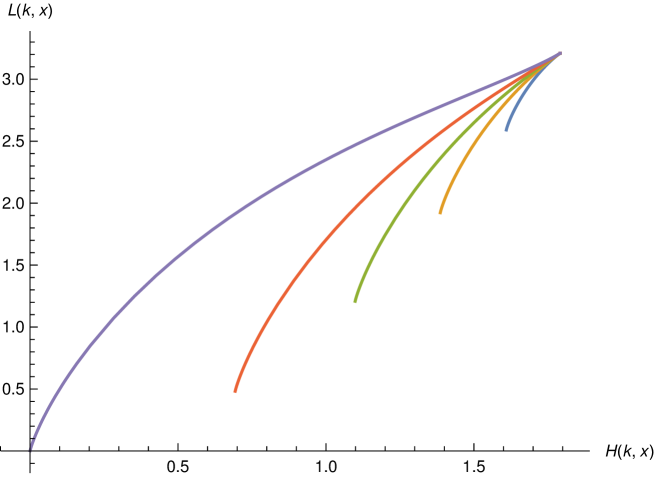
Figure 2: The locus of the points $(H,L)$ as $x$ varies over $[0,1/K]$, for the case $K=6$ and for each value of $k\in\{1,\dotsc,5\}$, with $k$ increasing towards the left. These loci are curves with lower end point $H=H(k,0)=\log(K-k)$, $L=L(k,0)=(\log(K-k))^{2}$ and upper end point $H=H(k,1/K)=\log K$, $L=L(k,1/K)=(\log K)^{2}$. The value $k=0$ yields a single point, just as the $k=K$ case does, coinciding with the upper end point of all other $(H,L)$ curves.

From now on we assume that $k\neq K$ and thus $H_{0}<\log K$. Then $y:=(1-kx)/(K-k)$ from the normalization constraint (6.37), so we can compute

$$H(k,x) :=H(q_{k,x})=-kx\log x-(K-k)y\log y,$$ (6.38)

$$L(k,x) :=L(q_{k,x})=kx(\log x)^{2}+(K-k)y(\log y)^{2}.$$ (6.39)

To obtain the global maximum of $L(k,x)$, a further optimization over $k\in\{1,\dotsc,K-1\}$ and $x\in[0,1/K)$ is required. The numerical calculations presented in the diagram in Fig. 2 suggest that $k=K-1$ yields the maximal value of $L$. To prove that this is actually true we will temporarily remove the restriction that $k$ be an integer and consider the entire range $k\in(0,K)$. Our analysis will show that keeping $H(k,x)$ fixed, $L(k,x)$ increases with $k$.

To keep $H$ fixed as $k$ changes, $x$ will have to change as well. For given $H_{0}\in[0,\log K)$, let $x(k)$ be the function of $k$ implicitly given by $H(k,x(k))=H_{0}$. We would like to know how $L(k,x(k))$ changes as a function of $k$. Taking the total derivative with respect to $k$ gives

$$\frac{d}{dk}H\big{\lparen}k,x(k)\big{\rparen} =\frac{\partial}{\partial k}H\big{\lparen}k,x(k)\big{\rparen}+\frac{\partial}{\partial x}H\big{\lparen}k,x(k)\big{\rparen}\,x^{\prime}(k)=0,$$ (6.40)

$$\frac{d}{dk}L\big{\lparen}k,x(k)\big{\rparen} =\frac{\partial}{\partial k}L\big{\lparen}k,x(k)\big{\rparen}+\frac{\partial}{\partial x}L\big{\lparen}k,x(k)\big{\rparen}\,x^{\prime}(k).$$ (6.41)

Solving the first equation for $x^{\prime}(k)$ and substituting the solution in the second equation gives

$$\frac{d}{dk}L\big{\lparen}k,x(k)\big{\rparen} =\frac{\partial}{\partial k}L\big{\lparen}k,x(k)\big{\rparen}-\frac{\partial}{\partial x}L\big{\lparen}k,x(k)\big{\rparen}\left.\frac{\partial}{\partial k}H\big{\lparen}k,x(k)\big{\rparen}\middle/\frac{\partial}{\partial x}H\big{\lparen}k,x(k)\big{\rparen}\right.$$

$$=\frac{1}{K-k}\left[\Big{\lparen}1+(K-2k)x\Big{\rparen}\Big{\lparen}\log\frac{1-kx}{K-k}-\log x\Big{\rparen}-2(1-Kx)\right],$$ (6.42)

where the second line follows by substituting the partial derivatives of $H(k,x)$ and $L(k,x)$ defined in eqs. 6.38 and 6.39.

Note that $z\geq\tanh z=(e^{2z}-1)/(e^{2z}+1)$ for any $z\geq 0$. By choosing $z:=(\log w)/2$ we get $\log w\geq 2(w-1)/(w+1)$ for $w\geq 1$. Next, since $x\leq 1/K$, we can take $w:=(1-kx)/(Kx-kx)\geq 1$ which gives

$$\log\frac{1-kx}{K-k}-\log x\geq 2\left.\left\lparen\frac{1-kx}{(K-k)x}-1\right\rparen\middle/\left\lparen\frac{1-kx}{(K-k)x}+1\right\rparen\right.=2\,\frac{1-Kx}{1+(K-2k)x}.$$ (6.43)

Inserting this in eq. 6.42 and noting that $1+(K-2k)x\geq 0$ for $x\leq 1/K$, we conclude that $dL(k,x(k))/dk\geq 0$, so $L(k,x(k))$ is increasing as a function of $k$ just as we intended to show.

Reverting back to integer values of $k$, we find that, for a fixed value of $H(k,x)$, the value of $L(k,x)$ is maximized when $k$ is the largest integer in the open interval $(0,K)$, namely $K-1$. Then $L_{\max}(H_{0})$, the maximum value of $L(k,x)$ subject to $H(k,x)=H_{0}$, see eq. 6.30, is given by $L(K-1,x)$ where $x$ is such that $H(K-1,x)=H_{0}$.

Finally, we have to perform a further maximization over $K$, for $K\leq d$. In a similar way as before $x$ becomes a function of $K$. We now show that the maximum of $L(K-1,x(K))$ under the constraints $H(K-1,x(K))=H_{0}$ and $K\leq d$ occurs for $K=d$. Solving the equation $0=\frac{d}{dK}H(K-1,x(K))$ for $x^{\prime}(K)$ and substituting the solution back into $\frac{d}{dK}L(K-1,x(K))$ shows after a fair bit of algebra that

$$\frac{d}{dK}L(K-1,x(K))=x(K)\Big{[}2+\log\big{\lparen}1-K+1/x(K)\big{\rparen}\Big{]},$$ (6.44)

which is clearly non-negative for $0\leq x(K)\leq 1/K$, hence $L(K-1,x(K))$ increases with $K$. We conclude that the overall maximum occurs for $K=d$, as we set out to prove.

The last statement of the lemma is now easily shown. From eq. 6.39 we infer that

$$L_{\max}(H_{0})-H_{0}^{2}=L(d-1,x)-H(d-1,x)^{2}=rx(1-rx)\big{\lparen}\log x-\log(1-rx)\big{\rparen}^{2},$$ (6.45)

where $r:=d-1$ and $x\in[0,1/d]$ satisfies $H(d-1,x)=H_{0}$. ∎

For $r=d-1$ and any $x\in[0,1/d]$, if $q_{r,x}$ is the probability distribution defined in eq. 6.36, we denote its Shannon entropy and the information variance by

$$s_{r}(x) :=H(q_{r,x})=-rx\log x-(1-rx)\log(1-rx),$$ (6.46)

$$w_{r}(x) :=V(q_{r,x})=L(q_{r,x})-H(q_{r,x})^{2}=rx(1-rx)\big{\lparen}\log x-\log(1-rx)\big{\rparen}^{2}.$$ (6.47)

In terms of these quantities, the condition in Lemma 14, under which a given function of the von Neumann entropy is concave on the set of qudit states, is expressed by the following theorem.

Theorem 16.

Let $h:\mathbb{R}\to\mathbb{R}$ be a twice-differentiable, monotonously increasing function. Then the function $f_{c}(\rho):=h(cH(\rho))$ with $c\geq 0$ and $\rho\in\mathcal{D}(\mathbb{C}^{d})$ is concave on $\mathcal{D}(\mathbb{C}^{d})$ if

$$c\,\frac{h^{\prime\prime}(cs_{r}(x))}{h^{\prime}(cs_{r}(x))}\leq\frac{1}{w_{r}(x)},$$ (6.48)

for all $0\leq x\leq 1/d$, where $r:=d-1$ and functions $s_{r}(x)$ and $w_{r}(x)$ are defined in eqs. 6.46 and 6.47.

6.1 Concavity of Entropy Power

In this section we use Theorem 16 to establish the first item of Theorem 6, namely, that the entropy power $E_{c}(\rho)=e^{cH(\rho)}$ of a state $\rho\in\mathcal{D}(\mathbb{C}^{d})$ is concave for $0\leq c\leq 1/(\log d)^{2}.$

Proof of Theorem 6 (concavity of $E_{c}$).

In this case we have $h(x)=\exp(x)$, so the condition (6.48) just translates to

$$c\leq 1/w_{d-1}(x),\quad 0\leq x\leq 1/d.$$ (6.49)

Therefore,

$$c\leq\Big{\lparen}\max_{0\leq x\leq 1/d}w_{d-1}(x)\Big{\rparen}^{-1}=:c_{\max}.$$ (6.50)

From the expression of $w_{r}$ follows a simple lower bound on the largest allowed value of $c$. Putting $y=rx$, with $0\leq y\leq(d-1)/d<1$,

$$w_{r}(x) =y(1-y)\big{\lparen}-\log r+\log y-\log(1-y)\big{\rparen}^{2}$$

$$=A(\log r)^{2}+B\log r+C,$$ (6.51)

where the coefficients $A,B,C$ of this quadratic polynomial in $\log r$ are bounded above as follows: $A:=y(1-y)\leq 1/4$, $B:=-2y(1-y)\big{\lparen}\log y-\log(1-y)\big{\rparen}\leq 1/2$, and $C:=y(1-y)\big{\lparen}\log y-\log(1-y)\big{\rparen}^{2}\leq 1/2$. Hence,

$$w_{r}(x)\leq(1+\log r)/2+(\log r)^{2}/4\quad\text{with }r=d-1,$$ (6.52)

and we obtain

$$c_{\max}\geq 1/\big{[}\big{\lparen}1+\log(d-1)\big{\rparen}/2+\big{\lparen}\log(d-1)\big{\rparen}^{2}/4\big{]}.$$ (6.53)

This bound becomes asymptotically exact in the limit of large $d$. Note that the right-hand side of eq. 6.53 is larger than $1/(\log d)^{2}$ for $d\geq 3$. For $d=2$, the right-hand side of eq. 6.53 is equal to 2 which is not larger than $1/(\log 2)^{2}\approx 2.0814$. However, for this case one can numerically evaluate the expression (6.50) for $c_{\max}$ to obtain the value $2.2767$, which is indeed greater than $1/(\log 2)^{2}$. ∎

From this we can also infer that for any probability distribution $p$ over $d$ elements, the function $E(p):=e^{cH(p)}$ is concave for $0\leq c\leq 1/(\log d)^{2}$.

Remark.

The fact that for $h(x):=\exp(x)$ the inequality (6.3) of Lemma 14 holds for any value of $c$ in the range $0\leq c\leq 1/(\log d)^{2}$ can also be proved using Theorem 8 and Lemma 15 of [RW15].

6.2 Concavity of Entropy Photon Number

In this section we use Theorem 16 to establish the second item of Theorem 6, namely, that the entropy photon number $N_{c}(\rho)$ of a qudit, defined by eq. 3.3, is concave for $0\leq c\leq 1/(d-1)$.

Proof of Theorem 6 (concavity of $N_{c}$).

In this case the calculations are more complicated because $h$ is not given directly but as the inverse of a function: $h=g^{-1}$, where

$$g(x)=-x\log(x)+(1+x)\log(1+x).$$ (6.54)

The derivatives of $h$ are given by

$$h^{\prime}(x) =\frac{1}{g^{\prime}(h(x))}=\frac{1}{\log(1+1/h(x))},$$ (6.55)

$$h^{\prime\prime}(x) =\frac{1}{\big{\lparen}h(x)+h^{2}(x)\big{\rparen}\big{[}\log(1+1/h(x))\big{]}^{3}}.$$ (6.56)

Defining the function

$$k(x)=x(1+x)\big{\lparen}\log(x)-\log(1+x)\big{\rparen}^{2},$$ (6.57)

we have $h^{\prime}(x)/h^{\prime\prime}(x)=k(h(x))$. The function $k$ is monotonously increasing, concave, and ranges from 0 to 1. The condition on $c$ becomes

$$g^{-1}(cs_{r}(x))\geq k^{-1}(cw_{r}(x)).$$ (6.58)

If we define the variables $y$ and $z$ according to

$$g(y)=cs_{r}(x),\qquad k(z)=cw_{r}(x),$$ (6.59)

the condition is $y\geq z$. If we now exploit the monotonicity of $k$, this condition is equivalent to $k(y)\geq k(z)=cw_{r}(x)$. We therefore require that

$$g(y)=cs_{r}(x)\,\,\mbox{ implies }\,\,k(y)\geq cw_{r}(x).$$ (6.60)

We will show that this holds for $c\leq 1/a=1/(d-1)$. In Fig. 3 we depict the graph of $k(y)$ versus $g(y)$. The graph seems to indicate that the resulting curve is concave and monotonously increasing; that this is actually true follows from the easily checked fact that the function $k^{\prime}/g^{\prime}=(1+2x)\big{\lparen}\log(1+x)-\log x\big{\rparen}-2$, representing the slope of the curve, is positive and decreasing. The condition (6.60) amounts to the statement that any point $(cs_{r}(x),cw_{r}(x))$ lies in the area below this curve. Hence if the condition is satisfied for a certain value of $c$, then it is also satisfied for any smaller positive value of $c$. Therefore, we only need to prove eq. 6.60 for $c=1/(d-1)$.

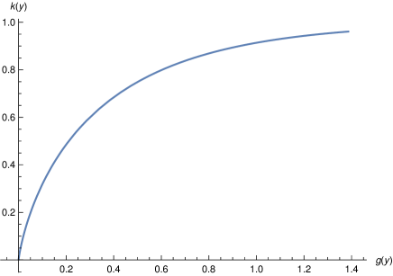
Figure 3: Parametric plot of $k(y)$ versus $g(y)$.

The formal similarities between $g$ and $s_{r}$ and between $k$ and $w_{r}$ let us define two interpolating functions $g_{1}(x,b)$ and $k_{1}(x,b)$ as a function of the original $x$ and an interpolation parameter $b$:

$$g_{1}(x,b) =-x\log x+(1+bx)\frac{\log(1+bx)}{b},$$ (6.61)

$$k_{1}(x,b) =x(1+bx)\big{\lparen}\log x-\log(1+bx)\big{\rparen}^{2}.$$ (6.62)

Let $\mathcal{S}$ indicate the domain of $g_{1}$ and $k_{1}$, which is $b\in[1-d,1]$ and $x\in[0,1/d]$, as before. To ensure continuity of $g_{1}$ at $b=0$, we define $g_{1}(x,0)$ to be its limit value $\lparen-x\log x+x\rparen$. Hence, we have the correspondences

$$s_{r}(x)/(d-1) =g_{1}(x,1-d), g(x)=g_{1}(x,1),$$ (6.63)

$$w_{r}(x)/(d-1) =k_{1}(x,1-d), k(x)=k_{1}(x,1).$$ (6.64)

The condition (6.60) is therefore satisfied if a continuous path $x(b)$ exists (from $x(1-d)=x$ to $x(1)=y$) such that $g_{1}(x(b),b)$ remains constant and $k_{1}(x(b),b)$ increases with $b$. As in the proof of Lemma 15 this requires the positivity of

$$\frac{d}{db}k_{1}(x(b),b) =\frac{\partial}{\partial b}k_{1}(x(b),b)-\frac{\partial}{\partial x}k_{1}(x(b),b)\left.\frac{\partial}{\partial b}g_{1}(x(b),b)\middle/\frac{\partial}{\partial x}g_{1}(x(b),b)\right.$$

$$=\frac{1}{b^{2}}\Bigl{[}bx\big{\lparen}2+\log x+bx(\log x)^{2}\big{\rparen}$$

$$\quad+(1+bx)^{2}\big{\lparen}\log(1+bx)\big{\rparen}^{2}$$

$$\quad-\Big{\lparen}2+bx+(1+2bx+2b^{2}x^{2})\log x\Big{\rparen}\log(1+bx)\Bigr{]}.$$ (6.65)

Let us introduce the variable $u=1+bx$. In $\mathcal{S}$ we have $(1-b)x\leq 1$ so that $x\leq u$; furthermore, $b\leq 1$ and $x\leq 1/d$, so that $u\leq 1+1/d$. The second factor can now be written more succinctly as

$$(u-1)\left(2+\log x+(u-1)(\log x)^{2}\right)+u^{2}(\log u)^{2}-(1+u+(1-2u+2u^{2})\log x)\log u$$

$$={} (u-1)^{2}\log x(\log x-\log u)+u^{2}(\log u)^{2}$$

$$+2(u-1)-(u+1)\log u-(1-u+u^{2}\log u)\log x.$$ (6.66)

The first two terms are clearly non-negative. The factor $1-u+u^{2}\log u$ is non-negative too, as can be seen from the inequality $1-\exp(-v)\leq v\leq v\exp(v)$ applied to $v=\log u$. Furthermore, $\log x\leq\log(1/d)\leq\log(1/2)\leq-1/2$, so that the last term is bounded below by $(1-u+u^{2}\log u)/2$. It is therefore left to show that $2(u-1)-(u+1)\log u+(1-u+u^{2}\log u)/2$ is non-negative.

For $0<u\leq 1$ we can exploit the inequality $\log u\leq 2(u-1)/(u+1)$, so that we obtain $2(u-1)-(u+1)\log u\geq 0$. The remaining term is non-negative too, as we have just showed.

For $1\leq u\leq 1+1/d$ we exploit instead the inequality $\log u\leq u-1$. Then based on the fact that in this range $(u-1)^{2}-3<0$

$$2(u-1)-(u+1)\log u+(1-u+u^{2}\log u)/2$$

$$=\frac{1}{2}\Big{\lparen}3(u-1)+\big{\lparen}(u-1)^{2}-3\big{\rparen}\log u\Big{\rparen}$$

$$\geq\frac{1}{2}\Big{\lparen}3(u-1)+\big{\lparen}(u-1)^{2}-3\big{\rparen}(u-1)\Big{\rparen}$$

$$=(u-1)^{3}/2\geq 0.$$ (6.67)

This shows that $k_{1}(x(b),b)$ indeed increases with $b$, whence condition (6.60) holds for $c=1/(d-1)$ and, by a previous argument, for $c\leq 1/(d-1)$. In other words, we have shown that the function $g^{-1}(cH(\rho))$ is concave for $0<c\leq 1/(d-1)$. As this includes the value $c=1/d$, the photon number is concave. ∎

7 Bounds on minimum output entropy and Holevo capacity

As an application of our results we now consider the class of quantum channels $\mathcal{E}_{a,\sigma}:\mathcal{D}(\mathbb{C}^{d})\to\mathcal{D}(\mathbb{C}^{d})$ obtained from the partial swap channel $\mathcal{E}_{a}$ from eq. 4.9 by fixing the second input state $\sigma$ (see Fig. 4). Such channels are parameterized by a variable $a\in[0,1]$ and a quantum state $\sigma\in\mathcal{D}(\mathbb{C}^{d})$, and act as follows:

$$\mathcal{E}_{a,\sigma}(\rho):=\rho\boxplus_{a}\sigma.$$ (7.1)

Figure 4: A schematic representation of the channel $\mathcal{E}_{a,\sigma}$ defined in eq. 7.1.

For example, for the choice $\sigma=I/d$ (the completely mixed state) the channel $\mathcal{E}_{a,\sigma}$ is just the quantum depolarizing channel with parameter $a$. If $\sigma=\delta|0\rangle\langle 0|+(1-\delta)|1\rangle\langle 1|\in\mathcal{D}(\mathbb{C}^{2})$ for some $\delta\in[0,1]$, then $\mathcal{E}_{a,\sigma}$ is a qubit channel whose output density matrix is

$$\begin{pmatrix}ar_{00}+(1-a)\delta&r_{01}(a-i\sqrt{a(1-a)}(1-2\delta))\\ r_{01}(a+i\sqrt{a(1-a)}(1-2\delta))&ar_{11}+(1-a)(1-\delta)\end{pmatrix}$$ (7.2)

for any input qubit state $\rho:=\sum_{i,j=0}^{1}r_{ij}|i\rangle\langle j|$.

An important characteristic quantity for any quantum channel $\mathcal{E}$ is its minimum output entropy, which is defined as

$$H_{\min}\lparen\mathcal{E}\rparen:=\min_{\rho}H\lparen\mathcal{E}(\rho)\rparen.$$ (7.3)

Lower bounds on this quantity for the class of channels $\mathcal{E}_{a,\sigma}$ can be obtained by using our EPIs and EPnI. In fact, the inequalities of Corollary 7 give various lower bounds on the output entropy of the channel $\mathcal{E}_{a,\sigma}$ (i.e. the entropy of any output state) in terms of the entropy $H(\rho)$ of an input state $\rho$:

$$H\lparen\mathcal{E}_{a,\sigma}(\rho)\rparen \geq aH(\rho)+(1-a)H(\sigma),$$ (7.4)

$$H\lparen\mathcal{E}_{a,\sigma}(\rho)\rparen \geq\frac{1}{c}\log\Big{[}a\exp(cH(\rho))+(1-a)\exp(cH(\sigma))\Big{]}, \text{with }c=1/(\log d)^{2},$$ (7.5)

$$H\lparen\mathcal{E}_{a,\sigma}(\rho)\rparen \geq\frac{1}{c}g\Big{[}ag^{-1}(cH(\rho))+(1-a)g^{-1}(cH(\sigma))\Big{]}, \text{with }c=1/(d-1).$$ (7.6)

Since the above bounds are of the form $H\lparen\mathcal{E}_{a,\sigma}(\rho)\rparen\geq G\lparen H(\rho)\rparen$, for some function $G$, we have

$$H_{\min}\lparen\mathcal{E}_{a,\sigma}\rparen \geq\min_{\rho}G\lparen H(\rho)\rparen$$

$$=\min_{0\leq H_{0}\leq\log d}G(H_{0}).$$ (7.7)

In Fig. 5 we have plotted the bounds $G(H_{0})$ for two illustrative cases, the three curves corresponding to the three choices of the function $G$ as given by the right-hand sides of eqs. 7.4, 7.5 and 7.6. For the qubit ($d=2$) case we actually have a tight lower bound

$$H\lparen\mathcal{E}_{a,\sigma}(\rho)\rparen\geq\ell\Big{[}a\ell^{-1}\big{\lparen}H(\rho)\big{\rparen}+(1-a)\ell^{-1}\big{\lparen}H(\sigma)\big{\rparen}\Big{]}$$ (7.8)

where $\ell(r)$ is the entropy of a qubit state whose Bloch vector has length $r$, see eq. A.5 in Appendix A. This bound follows from eq. A.14 in Appendix A and is also shown in Fig. 5.

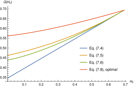
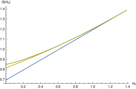
Figure 5: Plots of bounds $G$ from eq. 7.7 for the channel $\mathcal{E}_{1/2,\sigma}(\rho)$, where $\sigma$ is the maximally mixed state $\sigma=I/d$ in dimensions $d=2$ (left panel) and $d=4$ (right panel). The blue curves represent the bound (7.4) obtained from eq. 3.6, the orange curves represent the bound (7.5) obtained from the entropy power inequality (3.7), and the green curves represent the bound (7.6) obtained from the entropy photon number inequality (3.8). For $d=2$, the optimal bound (7.8) is given by the pink curve in the left panel. While neither of the bounds in eqs. 7.4, 7.5 and 7.6 is optimal for this channel, the numerics suggest that the entropy photon number inequality is the best out of the three when $d\geq 4$. For $d=2$, however, the entropy power inequality (7.5) yields a better bound.

These bounds imply lower bounds on the minimum output entropy $H_{\min}\lparen\mathcal{E}_{a,\sigma}\rparen$, which in turn allow us to obtain upper bounds on the product-state classical capacity of $\mathcal{E}_{a,\sigma}$. The latter is the capacity evaluated in the limit of asymptotically many independent uses of the channel, under the constraint that the inputs to multiple uses of the channel are necessarily product states. The Holevo-Schumacher-Westmoreland (HSW) [Hol98, SW97] theorem establishes that the product-state capacity of a memoryless quantum channel $\mathcal{E}$ is given by its Holevo capacity $\chi(\mathcal{E})$:

$$\chi(\mathcal{E}):=\max_{\{p_{i},\rho_{i}\}}\bigg{\{}H\Big{\lparen}\sum_{i}p_{i}\mathcal{E}(\rho_{i})\Big{\rparen}-\sum_{i}p_{i}H\big{\lparen}\mathcal{E}(\rho_{i})\big{\rparen}\bigg{\}},$$ (7.9)

where the maximum is taken over all ensembles $\{p_{i},\rho_{i}\}$ of possible input states $\rho_{i}$ occurring with probabilities $p_{i}$. Using the above expression, and the fact that $H(\omega)\leq\log d$ for any $\omega\in\mathcal{D}(\mathbb{C}^{d})$, we obtain the following simple bound:

$$\chi(\mathcal{E})\leq\log d-\min_{\rho}H\big{\lparen}\mathcal{E}(\rho)\big{\rparen},$$ (7.10)

where the minimum is taken over all possible inputs to the channel. Applying this bound to the channel $\mathcal{E}_{a,\sigma}$ for any $a\in[0,1]$ and $\sigma\in\mathcal{D}(\mathbb{C}^{d})$ and using eq. 7.4 we infer that

$$\chi(\mathcal{E}_{a,\sigma}) \leq\log d-a\min_{\rho}H(\rho)-(1-a)H(\sigma)$$

$$=\log d-(1-a)H(\sigma).$$ (7.11)

For the case of the qubit channel introduced above, we thus obtain the bound

$$\chi(\mathcal{E}_{a,\sigma})\leq\log 2-(1-a)h(\delta),$$ (7.12)

where $h(\delta):=-\delta\log\delta-(1-\delta)\log(1-\delta)$ is the binary entropy. Even sharper bounds are possible by exploiting eqs. 7.5 and 7.6.

8 Summary and open questions

In this paper we establish a class of entropy power inequalities (EPIs) for $d$-level quantum systems or qudits. The underlying addition rule for which these inequalities hold, is given by a quantum channel acting on the product state $\rho\otimes\sigma$ of two qudits and yielding the state of a single qudit as output. We refer to this channel as a partial swap channel since its output interpolates between the states $\rho$ and $\sigma$ as the parameter $a$ on which it depends is changed from $1$ to $0$. We establish EPIs not only for the von Neumann entropy and the entropy power, but also for a large class of functions, which include the Rényi entropies and the subentropy. Moreover, for the subclass of partial swap channels for which one of the qudit states in the input is fixed, our EPI for the von Neumann entropy yields an upper bound on the Holevo capacity.

We would like to emphasize that the method that we employ to prove our EPIs is novel, in the sense that it does not mimic the proofs of the EPIs in the continuous-variable classical and quantum settings. Instead it relies solely on spectral majorization and concavity of certain functions.

8.1 Open questions

Our results lead to many interesting open questions; here we briefly mention some of them. For example, can a conditional version of the EPI (see [Koe15]) be proved for qudits? Can an optimal bound similar to eq. 7.8 be found also for $d>2$? Is it possible to generalize our quantum addition rule (4.17) for combining more than two states? Such a generalization has recently been obtained for three states [Ozo15], though the problem for four or more states is not yet fully resolved. More importantly, proving analogues of our EPI for three or more states (similar to the multi-input EPI of [DMLG15]) remains an interesting open question. Finally, is the partial swap channel that we define the unique channel resulting in an interpolation between the input states and yielding a non-trivial EPI (i.e., one that is not simply a statement of concavity)? According to [Ozo15], it is unique (up to the sign of $i$) in a certain class of channels.

In Section 7, we mentioned a simple application of our EPI to quantum Shannon theory. Considering the significance of the classical EPI in information theory and statistics, we expect that our EPIs will also find further applications.

Finally, it would be worth exploring whether our proof of the qudit analogue of the entropy photon number inequality can be generalized to establish the EPnI for the bosonic case (which is known to be an important open problem).

Appendix A Entropy power inequality for qubits

For the case of qubits ($d=2$), there is a simple proof of eq. 3.6 which exploits the Bloch-vector representation of a qubit state.

A.1 Qubit states and the Bloch sphere

It is known that the state $\rho$ of a qubit can be expressed in terms of its Bloch vector $\vec{r}$ as follows:

$$\rho=\frac{1}{2}(I+\vec{r}\cdot\vec{\sigma})=\frac{1}{2}(I+x\sigma_{x}+y\sigma_{y}+z\sigma_{z}),$$ (A.1)

where $\vec{r}:=(x,y,z)\in\mathbb{R}^{3}$ such that $\lvert\vec{r}\rvert:=\sqrt{x^{2}+y^{2}+z^{2}}\leq 1$. Here $\vec{r}\cdot\vec{\sigma}$ denotes a formal inner product between $\vec{r}$ and $\vec{\sigma}:=(\sigma_{x},\sigma_{y},\sigma_{z})$, with $\sigma_{x}$, $\sigma_{y}$ and $\sigma_{z}$ being the Pauli matrices. Moreover, the eigenvalues of the state $\rho$ can easily be seen to be given by $\frac{1}{2}(1\pm\lvert\vec{r}\rvert)$. Hence, its von Neumann entropy is simply

$$H(\rho)=h\big{\lparen}\tfrac{1}{2}(1+\lvert\vec{r}\rvert)\big{\rparen},$$ (A.2)

where $h(p):=-p\log p-(1-p)\log(1-p)$ is the binary entropy of $p\in[0,1]$ in nats. For $x\in[-1,1]$, let us define the function

$$\ell(x):=h\big{\lparen}\tfrac{1}{2}(1+x)\big{\rparen}.$$ (A.3)

One can easily see that $\ell$ is symmetric around the vertical axis and verify that

$$\ell^{\prime\prime}(x)=-\frac{1}{1-x^{2}}\leq 0,$$ (A.4)

so $\ell$ is concave (see Fig. 6). In terms of this function, eq. A.2 is given by

$$H(\rho)=\ell(\lvert\vec{r}\rvert).$$ (A.5)

Figure 6: A plot of the function $\ell$ defined in eq. A.3.

A.2 Proof of the qubit EPI

For a pair of qubit states $\rho_{1}$ and $\rho_{2}$, the first EPI of Corollary 7 is given by

$$H\big{\lparen}\rho_{1}\boxplus_{a}\rho_{2}\big{\rparen}\geq aH(\rho_{1})+(1-a)H(\rho_{2}),\qquad\forall\,a\in[0,1].$$ (A.6)

Below is a simple proof of the above inequality for the special case of qubits.

Proof.

Using eq. A.5, the inequality (A.6) can be expressed in terms of the function $\ell$ as follows:

$$\ell(r)\geq a\ell(r_{1})+(1-a)\ell(r_{2}),$$ (A.7)

where $r:=\lvert\vec{r}\rvert$, $r_{1}:=\lvert\vec{r}_{1}\rvert$, $r_{2}:=\lvert\vec{r}_{2}\rvert$, and $\vec{r}$, $\vec{r}_{1}$, $\vec{r}_{2}$ denote the Bloch vectors of the states $\rho_{1}\boxplus_{a}\rho_{2}$, $\rho_{1}$ and $\rho_{2}$, respectively. Recall from eq. 4.18 that $\vec{r}$ can be expressed in terms of $\vec{r}_{1}$ and $\vec{r}_{2}$ as follows:

$$\vec{r}=a\vec{r}_{1}+(1-a)\vec{r}_{2}+\sqrt{a(1-a)}(\vec{r}_{1}\times\vec{r}_{2}).$$ (A.8)

Since $\vec{r}_{1}$ and $\vec{r}_{2}$ are both perpendicular to $\vec{r}_{1}\times\vec{r}_{2}$, we get

$$\lvert\vec{r}\rvert^{2}=\vec{r}\cdot\vec{r}=a^{2}\lvert\vec{r}_{1}\rvert^{2}+(1-a)^{2}\lvert\vec{r}_{2}\rvert^{2}+2a(1-a)\vec{r}_{1}\cdot\vec{r}_{2}+a(1-a)\lvert\vec{r}_{1}\times\vec{r}_{2}\rvert^{2}.$$ (A.9)

If we denote by $\gamma\in[0,\pi]$ the angle between vectors $\vec{r}_{1}$ and $\vec{r}_{2}$, then $\vec{r}_{1}\cdot\vec{r}_{2}=\lvert\vec{r}_{1}\rvert\lvert\vec{r}_{2}\rvert\cos\gamma$ and $\lvert\vec{r}_{1}\times\vec{r}_{2}\rvert=\lvert\vec{r}_{1}\rvert\lvert\vec{r}_{2}\rvert\sin\gamma$, so eq. A.9 becomes

$$r^{2}=a^{2}r_{1}^{2}+(1-a)^{2}r_{2}^{2}+a(1-a)\lparen 2r_{1}r_{2}\cos\gamma+r_{1}^{2}r_{2}^{2}\sin^{2}\gamma\rparen.$$ (A.10)

Note that the right-hand side of the inequality (A.7) does not depend on the angle $\gamma$ between the vectors $\vec{r}_{1}$ and $\vec{r}_{2}$, so it suffices to prove eq. A.7 only for those values of $\gamma$ that minimize the left-hand side. Since $f(r)$ is a decreasing function of $r$ for $r\geq 0$ (see Fig. 6), we have to consider only those values of $\gamma$ that maximize $r$. From eq. A.10 we have that

$$r=\sqrt{a^{2}r_{1}^{2}+(1-a)^{2}r_{2}^{2}+a(1-a)r_{1}r_{2}\lparen 2\cos\gamma+r_{1}r_{2}\sin^{2}\gamma\rparen}$$ (A.11)

where $a,r_{1},r_{2}\in[0,1]$. To maximize this over $\gamma$, we only need to maximize the last term. Note that

$$2\cos\gamma+r_{1}r_{2}\sin^{2}\gamma\leq 2\cos\gamma+\sin^{2}\gamma\leq 2,$$ (A.12)

where the last inequality is tight if and only if $\gamma=0$. This gives a simple upper bound on $r$:

$$r\leq\sqrt{a^{2}r_{1}^{2}+(1-a)^{2}r_{2}^{2}+2a(1-a)r_{1}r_{2}}=ar_{1}+(1-a)r_{2}.$$ (A.13)

Since $\ell(r)$ is monotonically decreasing for $r\geq 0$, we get

$$\ell(r)\geq\ell\big{\lparen}ar_{1}+(1-a)r_{2}\big{\rparen}.$$ (A.14)

Note that this lower bound is independent of the parameter $\gamma$ and is tight (it becomes equality when $\gamma=0$). Recall from eq. A.4 that $f$ is concave (see also Fig. 6), so

$$\ell\big{\lparen}ar_{1}+(1-a)r_{2}\big{\rparen}\geq a\ell(r_{1})+(1-a)\ell(r_{2}).$$ (A.15)

By combining the last two inequalities, we get the desired result. ∎

References

- [Aud14] Koenraad M.R. Audenaert. Quantum skew divergence. Journal of Mathematical Physics, 55(11):112202, 2014. arXiv:1304.5935, doi:10.1063/1.4901039.
- [Bar86] Andrew R. Barron. Entropy and the central limit theorem. The Annals of Probability, 14(1):336–342, 1986. URL: http://projecteuclid.org/euclid.aop/1176992632.
- [Bec75] William Beckner. Inequalities in Fourier analysis. Annals of Mathematics, 102(1):159–182, Jul 1975. doi:10.2307/1970980.
- [Ber74] Patrick P. Bergmans. A simple converse for broadcast channels with additive white Gaussian noise. Information Theory, IEEE Transactions on, 20(2):279–280, Mar 1974. doi:10.1109/TIT.1974.1055184.
- [Bha97] Rajendra Bhatia. Matrix Analysis. Graduate Texts in Mathematics. Springer New York, 1997. URL: https://books.google.com/books?id=F4hRy1F1M6QC.
- [Bla65] Nelson M. Blachman. The convolution inequality for entropy powers. Information Theory, IEEE Transactions on, 11(2):267–271, Apr 1965. doi:10.1109/TIT.1965.1053768.
- [CLL16] Eric A. Carlen, Elliott H. Lieb, and Michael Loss. On a quantum entropy power inequality of Audenaert, Datta and Ozols. 2016. arXiv:1603.07043.
- [DCT91] Amir Dembo, Thomas M. Cover, and Joy A. Thomas. Information theoretic inequalities. Information Theory, IEEE Transactions on, 37(6):1501–1518, Nov 1991. doi:10.1109/18.104312.
- [DDJB14] Nilanjana Datta, Tony Dorlas, Richard Jozsa, and Fabio Benatti. Properties of subentropy. Journal of Mathematical Physics, 55(6):062203, 2014. arXiv:1310.1312, doi:10.1063/1.4882935.
- [DMG14] Giacomo De Palma, Andrea Mari, and Vittorio Giovannetti. A generalization of the entropy power inequality to bosonic quantum systems. Nature Photonics, 8(12):958–964, 2014. arXiv:1402.0404, doi:10.1038/nphoton.2014.252.
- [DMLG15] Giacomo De Palma, Andrea Mari, Seth Lloyd, and Vittorio Giovannetti. Multimode quantum entropy power inequality. Phys. Rev. A, 91(3):032320, Mar 2015. arXiv:1408.6410, doi:10.1103/PhysRevA.91.032320.
- [GES08] Saikat Guha, Baris I. Erkmen, and Jeffrey H. Shapiro. The entropy photon-number inequality and its consequences. In Information Theory and Applications Workshop, pages 128–130, Jan 2008. arXiv:0710.5666, doi:10.1109/ITA.2008.4601037.
- [GSE07] Saikat Guha, Jeffrey H. Shapiro, and Baris I. Erkmen. Classical capacity of bosonic broadcast communication and a minimum output entropy conjecture. Phys. Rev. A, 76(3):032303, Sep 2007. arXiv:0706.3416, doi:10.1103/PhysRevA.76.032303.
- [GSE08] Saikat Guha, Jeffrey H. Shapiro, and Baris I. Erkmen. Capacity of the bosonic wiretap channel and the entropy photon-number inequality. In IEEE International Symposium on Information Theory, 2008 (ISIT 2008), pages 91–95, Jul 2008. arXiv:0801.0841, doi:10.1109/ISIT.2008.4594954.
- [Guh08] Saikat Guha. Multiple-user quantum information theory for optical communication channels. PhD thesis, Dept. Electr. Eng. Comput. Sci., MIT, Cambridge, MA, USA, 2008. URL: http://hdl.handle.net/1721.1/44413.
- [Hir06] Tohya Hiroshima. Additivity and multiplicativity properties of some Gaussian channels for Gaussian inputs. Phys. Rev. A, 73(1):012330, Jan 2006. arXiv:quant-ph/0511006, doi:10.1103/PhysRevA.73.012330.
- [HJ12] Roger A. Horn and Charles R. Johnson. Matrix Analysis. Cambridge University Press, 2nd edition, 2012. URL: https://books.google.com/books?id=5I5AYeeh0JUC.
- [Hol98] Alexander S. Holevo. The capacity of the quantum channel with general signal states. Information Theory, IEEE Transactions on, 44(1):269–273, Jan 1998. arXiv:quant-ph/9611023, doi:10.1109/18.651037.
- [HV03] Peter Harremoës and Christophe Vignat. An entropy power inequality for the binomial family. Journal of Inequalities in Pure and Applied Mathematics, 4(5):93, 2003. URL: http://www.emis.ams.org/journals/JIPAM/article334.html?sid=334.
- [JRW94] Richard Jozsa, Daniel Robb, and William K. Wootters. Lower bound for accessible information in quantum mechanics. Phys. Rev. A, 49(2):668–677, Feb 1994. doi:10.1103/PhysRevA.49.668.
- [JY10] Oliver Johnson and Yaming Yu. Monotonicity, thinning, and discrete versions of the entropy power inequality. Information Theory, IEEE Transactions on, 56(11):5387–5395, Nov 2010. arXiv:0909.0641, doi:10.1109/TIT.2010.2070570.
- [KMN+07] Pieter Kok, William J. Munro, Kae Nemoto, Timothy C. Ralph, Jonathan P. Dowling, and Gerard J. Milburn. Linear optical quantum computing with photonic qubits. Rev. Mod. Phys., 79(1):135–174, Jan 2007. arXiv:quant-ph/0512071, doi:10.1103/RevModPhys.79.135.
- [Koe15] Robert Koenig. The conditional entropy power inequality for Gaussian quantum states. Journal of Mathematical Physics, 56(2):022201, 2015. arXiv:1304.7031, doi:10.1063/1.4906925.
- [KS13a] Robert König and Graeme Smith. Classical capacity of quantum thermal noise channels to within 1.45 bits. Phys. Rev. Lett., 110(4):040501, Jan 2013. arXiv:1207.0256, doi:10.1103/PhysRevLett.110.040501.
- [KS13b] Robert König and Graeme Smith. Limits on classical communication from quantum entropy power inequalities. Nature Photonics, 7(2):142–146, 2013. arXiv:1205.3407, doi:10.1038/nphoton.2012.342.
- [KS14] Robert König and Graeme Smith. The entropy power inequality for quantum systems. Information Theory, IEEE Transactions on, 60(3):1536–1548, Mar 2014. arXiv:1205.3409, doi:10.1109/TIT.2014.2298436.
- [Lie78] Elliott H. Lieb. Proof of an entropy conjecture of Wehrl. Communications in Mathematical Physics, 62(1):35–41, 1978. URL: http://projecteuclid.org/euclid.cmp/1103904300, doi:10.1007/BF01940328.
- [LMR14] Seth Lloyd, Masoud Mohseni, and Patrick Rebentrost. Quantum principal component analysis. Nature Physics, 10(9):631–633, 2014. arXiv:1307.0401, doi:10.1038/nphys3029.
- [Ozo15] Maris Ozols. How to combine three quantum states. 2015. arXiv:1508.00860.
- [PPV10] Yury Polyanskiy, Vincent H. Poor, and Sergio Verdú. Channel coding rate in the finite blocklength regime. Information Theory, IEEE Transactions on, 56(5):2307–2359, May 2010. doi:10.1109/TIT.2010.2043769.
- [Rén56] Alfréd Rényi. A characterization of Poisson processes. Magyar Tud. Akad. Mat. Kutató Int. Közl., 1(2):519–527, 1956.
- [Rén61] Alfréd Rényi. On measures of entropy and information. In Jerzy Neyman, editor, Proceedings of the Fourth Berkeley Symposium on Mathematical Statistics and Probability, Volume 1: Contributions to the Theory of Statistics, pages 547–561, Berkeley, California, 1961. University of California Press. URL: http://projecteuclid.org/euclid.bsmsp/1200512181.
- [Rio11] Olivier Rioul. Information theoretic proofs of entropy power inequalities. Information Theory, IEEE Transactions on, 57(1):33–55, Jan 2011. arXiv:0704.1751, doi:10.1109/TIT.2010.2090193.
- [RW15] David Reeb and Michael M. Wolf. Tight bound on relative entropy by entropy difference. Information Theory, IEEE Transactions on, 61(3):1458–1473, Mar 2015. doi:10.1109/TIT.2014.2387822.
- [SDM11] Naresh Sharma, Smarajit Das, and Siddharth Muthukrishnan. Entropy power inequality for a family of discrete random variables. In Information Theory Proceedings (ISIT), 2011 IEEE International Symposium on, pages 1945–1949. IEEE, Jul 2011. arXiv:1012.0412, doi:10.1109/ISIT.2011.6033891.
- [Sha48] Claude E. Shannon. A mathematical theory of communication. The Bell System Technical Journal, 27:623–656, Oct 1948. URL: http://cm.bell-labs.com/cm/ms/what/shannonday/shannon1948.pdf.
- [SS15] Yuri Suhov and Salimeh Y. Sekeh. Entropy-power inequality for weighted entropy. 2015. arXiv:1502.02188.
- [Sta59] A. J. Stam. Some inequalities satisfied by the quantities of information of Fisher and Shannon. Information and Control, 2(2):101–112, Jun 1959. doi:10.1016/S0019-9958(59)90348-1.
- [SW97] Benjamin Schumacher and Michael D. Westmoreland. Sending classical information via noisy quantum channels. Phys. Rev. A, 56(1):131–138, Jul 1997. doi:10.1103/PhysRevA.56.131.
- [VG06] Sergio Verdú and Dongning Guo. A simple proof of the entropy-power inequality. Information Theory, IEEE Transactions on, 52(5):2165–2166, May 2006. doi:10.1109/TIT.2006.872978.
- [vN50] John von Neumann. Functional Operators, Volume II: The geometry of orthogonal spaces. Princeton University Press, 1950. URL: https://books.google.co.uk/books?id=b3dOYQRBUk0C.
- [Zha02] Xingzhi Zhan. Matrix Inequalities, volume 1790 of Lecture Notes in Mathematics. Springer, 2002. URL: https://books.google.com/books?id=fvgxt6eYBl0C.