Unraveling the organization of the QCD tapestry

Abstract

I review some key aspects of the ongoing progress in our understanding of the infrared dynamics of the QCD Green’s functions, derived from the close synergy between Schwinger-Dyson equations and lattice simulations. Particular attention is dedicated to the elaborate nonperturbative mechanisms that endow the fundamental degrees of freedom (quarks and gluons) with dynamical masses. In addition, the recently established connection between the effective interaction obtained from the gauge sector of the theory and that needed for the veracious description of the ground-state properties of hadrons is briefly presented.

1 Introduction

Sixty years after their invention [1], Yang-Mills theories occupy the center stage of elementary particle physics, providing a fundamental description for an impressive array of physical phenomena. The remarkable property of asymptotic freedom makes these theories particularly attractive, and, in a sense, self-contained. However, while perturbation theory works well in their ultraviolet regime, the infrared dynamics represent a challenge of notorious complexity. In fact, in the case of QCD [2], the most characteristic phenomena, such as confinement, mass generation, and bound-state formation, are purely nonperturbative.

In this presentation we will focus on the paradigm-shifting picture that emerges for some of the aforementioned phenomena from the systematic study of Green’s functions within a global framework, where the analysis of the Schwinger-Dyson equations (SDEs) is complemented and refined by inputs obtained from large-volume lattice simulations.

The present study is restricted to the special case of the Landau gauge, where the vast majority of recent lattice simulations have been performed. The SDE part of the problem is addressed within the formalism obtained from the fusion between the pinch technique (PT) [3, 4, 5, 6, 7] and the background field method (BFM) [8], denoted simply as “PT-BFM” (for a representative sample of different approaches, see [9, 10, 11, 12, 13, 14, 15, 16, 17, 18, 19, 20]).

This presentation is organized as follows. In section 2 we review the PT-BFM formalism, and highlight its most salient features. Then, in section 3 we summarize the subtle filed-theoretic mechanism that leads to the gauge-invariant generation of a dynamical gluon mass. In section 4 we present a brief overview of the impressive coincidence achieved between SDE calculations and lattice simulations of the ghost propagator, while in section 5 we address some of the intricate issues surrounding the dynamical generation of the constituent quark masses. Then, in section 6 we review a recent ab-initio derivation of the interaction kernel that has been extensively used in the contemporary description of hadron phenomenology. Finally, in section 7 we summarize our conclusions.

2 The PT-BFM formalism: a powerful framework for studying SDEs

In what follows we will work exclusively in the Landau gauge, where the gluon propagator assumes the totally transverse form

$$i\Delta_{\mu\nu}(q)=-iP_{\mu\nu}(q)\Delta(q^{2});\qquad P_{\mu\nu}(q)=g_{\mu\nu}-q_{\mu}q_{\nu}/q^{2}\,.$$ (1)

The scalar form factor $\Delta(q^{2})$ is related to the all-order gluon self-energy $\Pi_{\mu\nu}(q)$. Specifically, as a consequence of the BRST symmetry, $\Pi_{\mu\nu}(q)$ is transverse, both perturbatively and nonperturbatively; one has then

$$q^{\mu}\Pi_{\mu\nu}(q)=0;\qquad\Pi_{\mu\nu}(q)=\Pi(q^{2})P_{\mu\nu}(q),$$ (2)

and $\Delta^{-1}(q^{2})=q^{2}+\Pi(q^{2})$. In addition, for later convenience, we introduce the inverse of the gluon dressing function, to be denoted by $J(q^{2})$, namely

$$\Delta^{-1}({q^{2}})=q^{2}J(q^{2}).$$ (3)

The nonperturbative dynamics of the gluon propagator are governed by the corresponding SDE. In particular, within the conventional formulation [21, 22], the gluon self-energy $\Pi_{\mu\nu}(q)$ is given by the fully dressed diagrams shown in Fig. 1. One longstanding difficulty with this equation is that it cannot be truncated in any obvious way without compromising the validity of Eq. (2). This happens because the conventional fully dressed vertices appearing in the diagrams of Fig. 1 satisfy complicated Slavnov-Taylor identities (STIs), and it is only after the inclusion of all diagrams that Eq. (2) may be enforced.

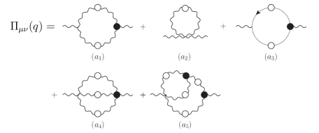
Figure 1: The conventional SDE of the standard gluon propagator ($QQ$). Black blobs represent fully dressed one-particle irreducible vertices, whereas the white ones denote fully dressed propagators.

Instead, the formulation of this SDE in the context of the PT-BFM formalism furnishes considerable advantages, because it allows for a systematic truncation that respects manifestly, and at every step, the crucial identity of Eq. (2). The deeper reason why such a truncation becomes possible may be traced back to the fact that the PT-BFM Green’s functions satisfy (by construction) Abelian-like Ward identities (WIs) instead of STIs. In particular, if we employ the BFM language and distinguish the gluon fields into background ($B$) and quantum ($Q$) ones, vertices such as $BQQ$, $B{\bar{c}}c$, and $BQQQ$, to be denoted by $\widetilde{\Gamma}_{\alpha\mu\nu}(q,r,p)$ , $\widetilde{\Gamma}_{\alpha}(q,r,-p)$, and $\widetilde{\Gamma}^{mnrs}_{\mu\nu\rho\sigma}(q,r,p,t)$, respectively, satisfy the simple WIs [23]

$$q^{\alpha}\widetilde{\Gamma}_{\alpha\mu\nu}(q,r,p)=i\Delta_{\mu\nu}^{-1}(r)-i\Delta_{\mu\nu}^{-1}(p),$$ (4)

$$q^{\alpha}\widetilde{\Gamma}_{\alpha}(q,r,-p)=D^{-1}(q+r)-D^{-1}(r),$$ (5)

and

$$q^{\mu}\widetilde{\Gamma}^{mnrs}_{\mu\nu\rho\sigma}(q,r,p,t) = f^{mse}f^{ern}\Gamma_{\nu\rho\sigma}(r,p,q+t)+f^{mne}f^{esr}\Gamma_{\rho\sigma\nu}(p,t,q+r)$$ (6)

$$+ f^{mre}f^{ens}\Gamma_{\sigma\nu\rho}(t,r,q+p).$$

These particular vertices (instead of the conventional ones) appear in the SDE of Fig. 2, which controls the self-energy $\widetilde{\Pi}_{\mu\nu}(q)$ of the the mixed background-quantum gluon propagator ($BQ$), denoted by $\widetilde{\Delta}(q^{2})$. Consequently, it is relatively straightforward to prove the block-wise transversality of $\widetilde{\Pi}_{\mu\nu}(q)$, namely [23]

$$q^{\mu}[(a_{1})+(a_{2})]_{\mu\nu}=0;\qquad q^{\mu}[(a_{3})+(a_{4})]_{\mu\nu}=0;\qquad q^{\mu}[(a_{5})+(a_{6})]_{\mu\nu}=0.$$ (7)

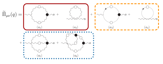
Figure 2: The SDE obeyed by the $QB$ gluon propagator. Black blobs represents fully dressed 1-PI vertices; the small gray circles appearing on the external legs (entering from the right, only!) are used to indicate background gluons. The diagrams contained in each box form individually transverse subsets.

From Eq. (2) it is clear that the SDE of $\widetilde{\Delta}(q^{2})$ contains inside its defining diagrams the full propagator $\Delta(q^{2})$; therefore, in that sense, it cannot be considered as a dynamical equation for neither $\widetilde{\Delta}(q^{2})$ nor $\Delta(q^{2})$. At this point a crucial identity relating $\Delta(q^{2})$ and $\widetilde{\Delta}(q^{2})$ [24, 25] enters into the game. Specifically, one has that

$$\Delta(q^{2})=[1+G(q^{2})]\widetilde{\Delta}(q^{2}),$$ (8)

where $G(q^{2})$ is the $g_{\mu\nu}$ co-factor of a certain two-point function that originates from the ghost sector of the theory.

The fundamental observation put forth in a series of works [23, 26, 27] is that one may use the SDE for $\widetilde{\Delta}(q^{2})$, take advantage of its improved truncation properties, and then convert it to an equivalent equation for $\Delta(q^{2})$ (the propagator simulated on the lattice) by means of the special relation given in Eq. (8). Thus, the PT-BFM version of the SDE for the conventional gluon propagator reads

$$\Delta^{-1}(q^{2}){P}_{\mu\nu}(q)=\frac{q^{2}{P}_{\mu\nu}(q)+i\,\sum_{i=1}^{6}(a_{i})_{\mu\nu}}{1+G(q^{2})}.$$ (9)

3 Dynamical gluon mass generation

The possibility that Yang-Mills theories generate dynamically a gluon mass was first proposed and explored in the early eighties [3, 28, 29], and has attracted particular attention in recent years, mainly due an accumulation of hard evidence obtained from large-volume lattice simulations, both in SU(3) [30, 31, 32, 33] and in SU(2) [34, 35, 36, 37] (for a different lattice approach, see [38]).

What these simulations reveal is that the Landau gauge gluon propagator saturates in the deep infrared at a fixed nonvanishing value, as shown on the left panel of Fig. 3, which is the smoking gun signal for gluon mass generation. A conclusive demonstration of how this may happen at the level of the gluon SDE within the PT-BFM framework has been given in [39].

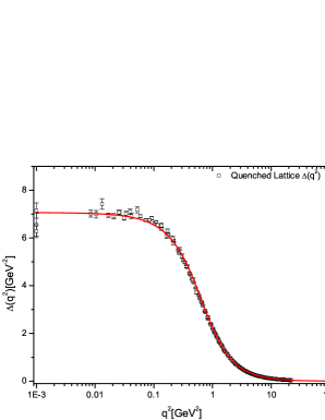
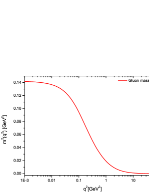
Figure 3: The quenched lattice gluon propagator $\Delta(q^{2})$ (left panel), and the corresponding gluon mass (right panel).

From the kinematic point of view we will describe the transition from a massless to a massive gluon propagator by implementing the replacement (in Euclidean space)

$$\Delta^{-1}(q^{2})=q^{2}J(q^{2})\quad\longrightarrow\quad\Delta^{-1}(q^{2})=q^{2}J(q^{2})+m^{2}(q^{2}),$$ (10)

where $m^{2}(q^{2})$ is the (momentum-dependent) dynamically generated mass, with the property that $m^{2}(0)>0$; evidently, $\Delta^{-1}(0)=m^{2}(0)$.

The actual field-theoretic mechanism that permits the generation of the term $m^{2}(q^{2})$ can be traced back to the seminal work of Schwinger [40, 41], which may be summarized in the statement that the vacuum polarization of a gauge boson that is massless at the level of the original Lagrangian may develop a massless pole, whose residue will be eventually identified with $m^{2}(0)$. In the case of Yang-Mills theories, the origin of the aforementioned poles is due to purely nonperturbative dynamics: for sufficiently strong binding, the mass of certain (colored) bound states may be reduced to zero [42, 43, 44, 45, 46]. As has been shown in [47] through a detailed study of the Bethe-Salpeter equation that controls the formation of such a composite massless pole, this dynamical scenario is indeed realized.

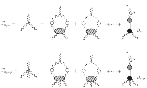
Figure 4: The SDEs for the full three and four gluon vertices in the presence of their corresponding pole parts.

In addition to triggering the Schwinger mechanism, these bound-state poles act as composite, longitudinally coupled Nambu-Goldstone bosons, maintaining gauge invariance; notice, however, that they differ from ordinary Nambu-Goldstone bosons as far as their origin is concerned, since they are not associated with the spontaneous breaking of any continuous symmetry. In particular, gauge invariance requires that the replacement described schematically in Eq. (10) be accompanied by a simultaneous replacement of all relevant vertices by

$$\widetilde{\Gamma}\quad\longrightarrow\quad\widetilde{\Gamma}^{\prime}=\widetilde{\Gamma}+\widetilde{V},$$ (11)

where $\widetilde{V}$ contains the aforementioned massless poles (see Fig. 4), and guarantees that the new vertex $\widetilde{\Gamma}^{\prime}$ satisfies the same WIs as $\widetilde{\Gamma}$, but now replacing the gluon propagators appearing on their rhs by massive ones. For example, in order to maintain Eq. (4) intact, the corresponding $\widetilde{V}$ must satisfy the WI

$$q^{\alpha}\widetilde{V}_{\alpha\mu\nu}(q,r,p)=m^{2}(r^{2})P_{\mu\nu}(r)-m^{2}(p^{2})P_{\mu\nu}(p);$$ (12)

similarly, when contracted with respect to the other two momenta, $\widetilde{V}_{\alpha\mu\nu}(q,r,p)$ satisfies the STIs necessary to enforce the validity of the corresponding STIs satisfied by $\widetilde{\Gamma}_{\alpha\mu\nu}(q,r,p)$, but now with massive instead of massless gluon propagators on the rhs.

The fact that the massless poles must be longitudinally coupled is reflected at the level of $\widetilde{\Gamma}^{\prime}$ through the condition

$$P^{\alpha^{\prime}\alpha}(q)P^{\mu^{\prime}\mu}(r)P^{\nu^{\prime}\nu}(p)\widetilde{V}_{\alpha^{\prime}\mu^{\prime}\nu^{\prime}}(q,r,p)=0,$$ (13)

and a exactly analogous relation for the four-gluon $\widetilde{V}_{\alpha\mu\nu\rho}(q,r,p,t)$. These latter conditions guarantee that the massless poles decouple completely from the on-shell $S$-matrix or other physical observables. Moreover, when Eq. (13) is combined with Eq. (12) and the additional STIs not reported here, one obtains the exact closed expression for $\widetilde{V}_{\alpha^{\prime}\mu^{\prime}\nu^{\prime}}(q,r,p)$ [48].

The inclusion of the aforementioned vertices into the gluon SDE leads to its separation into two integral equations of the generic form

$$J_{m}(q^{2}) = 1+\int_{k}{\cal K}_{1}(q^{2},m^{2},\Delta_{m}),$$

$$m^{2}(q^{2}) = \int_{k}{\cal K}_{2}(q^{2},m^{2},\Delta_{m}),$$ (14)

such that $q^{2}{\cal K}_{1}(q^{2},m^{2},\Delta_{m})\to 0$, as $q^{2}\to 0$, whereas ${\cal K}_{2}(q^{2},m^{2},\Delta_{m})\neq 0$ in the same limit, precisely because it includes the $1/q^{2}$ terms contained inside the $\widetilde{V}$ terms. This set of equations bares a close analogy to those studied in the case of the more familiar phenomenon of quark mass generation; in particular, $m^{2}(q^{2})$ plays the role of the quark mass function (denoted by $B(p^{2})$ in Eq. (22)).

The explicit closed form of the integral equation that determines $m^{2}(q^{2})$, together with a variety of related theoretical considerations, have been presented in a series of works [49, 50, 51]. The upshot is that one obtains a dynamical gluon mass of the form shown on the right panel of Fig. 3, whose functional dependence may be fitted by

$$m^{2}(q^{2})=\frac{m_{0}^{2}}{1+(q^{2}/{\mathcal{M}}^{2})^{1+p}}\,,$$ (15)

with $m_{0}=375\,\mbox{MeV}$, $p=0.11$ and ${\mathcal{M}}=431\,\mbox{MeV}$.

The nontrivial momentum dependence of the gluon mass is mainly responsible for the fact that, contrary to a propagator with a constant mass, the gluon propagator of Fig. 3 displays an inflection point. It turns out that the presence of such a feature is a sufficient condition for the spectral density of the gluon propagator, $\rho$, to be non-positive definite.

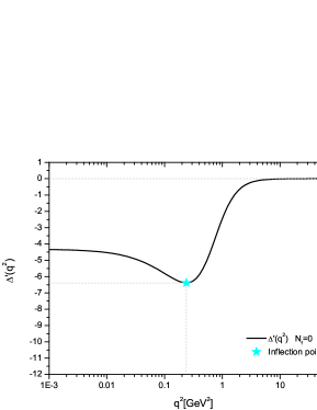
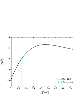
Figure 5: The first and second derivatives of the gluon propagator.

Specifically, the Källén-Lehman representation of the gluon propagator reads

$$\Delta(q^{2})=\int^{\infty}_{0}d\sigma\frac{\rho(\sigma)}{q^{2}+\sigma}\,,$$ (16)

and if $\Delta(q^{2})$ has an inflection point at $q^{2}_{\star}$, then its second derivative vanishes at that point (see Fig. 5), namely [52]

$$\Delta^{\prime\prime}(q^{2}_{\star})=2\int^{\infty}_{0}d\sigma\frac{\rho(\sigma)}{(q^{2}_{\star}+\sigma)^{3}}=0\,.$$ (17)

Given that $q^{2}_{\star}>0$, then $\rho(\sigma)$ is forced to reverse sign at least once. The non-positivity of $\rho(\sigma)$, in turn, may be interpreted as a signal of confinement (see [53], and references therein), since the breeching of the axiom of reflection positivity excludes the gluon from the Hilbert space of observables states (for related works, see [54, 55, 56, 57, 58, 59, 60]).

As can be seen in Fig. 5, the first derivative of $\Delta(q^{2})$ displays a minimum at $q^{2}_{\star}=0.238\,\mbox{GeV}^{2}$, and, consequently, the second derivative vanishes at that same point.

4 Ghost sector

The nonperturbative behavior of the ghost propagator, $D(p^{2})$, has been the focal point of intensive studies, because in the past it had been linked to a certain confinement scenario [9], whose realization required that the corresponding ghost dressing function, $F(p^{2})=p^{2}D(p^{2})$, should diverge at $p^{2}=0$. However, a plethora of high quality lattice simulations (for SU(3) [31, 32, 30, 33] and for SU(2) [34, 35, 36, 37]) have conclusively established that $F(p^{2})$ is finite at the origin. In fact, the finiteness of $F(p^{2})$ is tightly interwoven with the massiveness of the gluon, because it is precisely the presence of the gluon mass that tames the logarithm associated with $F(p^{2})$, and prevents it from diverging in the infrared [39].

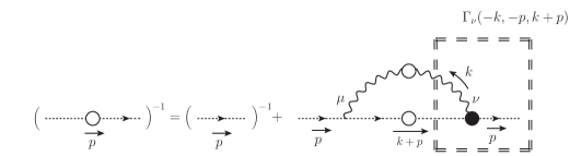
Figure 6: The SDE for the ghost propagator given by Eq. (18). The white blobs represent the fully dressed gluon and ghost propagators, while the black blob denotes the dressed ghost-gluon vertex.

Even though the finiteness of $F(p^{2})$ may be explained qualitatively in the above relatively simple terms, a more strenuous effort is required in order to obtain from the corresponding SDE the full curve of $F(p^{2})$ observed on the lattice.

The SDE for the ghost propagator is diagrammatically represented in the Fig. 6, and assumes the form

$$iD^{-1}(p^{2})=ip^{2}-g^{2}C_{\rm{A}}\int_{k}\Gamma_{\mu}^{[0]}(k,-k-p,p)\Delta^{\mu\nu}(k)\Gamma_{\nu}(-k,-p,k+p)D(k+p)\,.$$ (18)

In the above equation $C_{A}$ represents the Casimir eigenvalue of the adjoint representation ($N$ for $SU(N)$), $d=4-\epsilon$ is the space-time dimension, and we have introduced the integral measure

$$\int_{k}\equiv\frac{\mu^{\epsilon}}{(2\pi)^{d}}\!\int\!\mathrm{d}^{d}k,$$ (19)

with $\mu$ the ’t Hooft mass. The vertex $\Gamma_{\nu}(-k,-p,k+p)$ is the fully dressed ghost-gluon vertex, whose tensorial decomposition is given by ($r=k+p$)

$${\Gamma}_{\nu}(-k,-p,r)=A(-k,-p,r)\,p_{\nu}+B(-k,-p,r)\,k_{\nu}\,;$$ (20)

at tree-level, the two form factors assume the values $A^{[0]}(-k,-p,r)=1$ and $B^{[0]}(-k,-p,r)=0$, reproducing the standard bare vertex $\Gamma^{[0]}_{\nu}=p_{\nu}$. Clearly, due to the full transversality of $\Delta_{\mu\nu}(k)$, any reference to the form factor $B$ disappears from the ghost SDE of Eq. (18), and one obtains.

$$F^{-1}(p^{2})=1+ig^{2}C_{\rm{A}}\int_{k}\,\left[1-\frac{(k\cdot p)^{2}}{k^{2}p^{2}}\right]A(-k,-p,k+p)\Delta(k)D(k+p)\,.$$ (21)

The dependence of this equation on both $\Delta(k)$ and $A(-k,-p,k+p)$ is just another example of the perennial difficulty inherent to the SDE framework, namely the fact that, in principle, all Green’s functions of the theory are coupled to each other. In the case at hand, $\Delta(k)$ is known from the lattice (Fig. 3), and there is no need to resort to its own SDE. However, $A$ is more problematic, since there are no lattice data for the kinematic configuration relevant to this problem (for SU(2), see [61, 62, 63]). The obvious easy way out, namely the use of the tree-level value for $A$ is quantitatively insufficient: one obtains the result shown on the right panel of Fig. 7 (blue dashed curve), which, even though qualitatively correct, it is clearly considerably suppressed compared to the lattice data.

To ameliorate this situation, an approximate version of the SDE equation that controls the evolution of $A$ has been considered in [64], in the special kinematic limit $p\to 0$ (for a related study, see [65]); the result for $A(-k,0,k)$ is shown in the left panel of Fig. 7.

Even though the increase with respect to the tree level value is not too dramatic, the peak of $A(-k,0,k)$ at around 1 GeV turns out to be just right: when coupled with Eq. (21), a considerable enhancement of the resulting $F(p^{2})$ is produced, due to the nonlinear nature of this system of integral equations. As shown in the right panel of Fig. 7, one may actually reproduce the lattice data very accurately, using the correct value for the strong coupling $\alpha_{s}$ [66, 67].

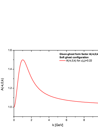
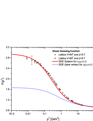
Figure 7: Left panel: The numerical result for the form factor $A(-k,0,k)$ in the soft ghost configuration (red continuous line) [64]. Right panel: The $F(p^{2})$ obtained from the ghost SDE with a bare ghost-gluon vertex (blue dashed curve) and the corresponding solution when the $A(-k,0,k)$ is used (red continuous line) , using in both cases $\mu=4.3$ GeV and $\alpha_{s}(\mu)=0.22$. The lattice data are from Ref. [31].

5 Quark sector

It is well known that the nonperturbative mechanism that endows quarks with their constituent masses accounts for about $98\%$ of the visible matter in the Universe. In fact, it has often been denominated as the most efficient mass generating mechanism known, practically generating masses from nothing (see [53] and references therein). This fundamental phenomenon (and the related dynamical breaking of the chiral symmetry) is encoded in the SDE of the quark propagator, know also as quark “gap equation”.

The standard decomposition of the quark propagator, $S(p)$, is given by [21]

$$S^{-1}(p)=A(p^{2})\,/{p}-B(p^{2})\mathbb{I}=A(p^{2})[/{p}-{\mathcal{M}}(p^{2})\mathbb{I}]\,,$$ (22)

where $\mathbb{I}$ is the identity matrix, and $\mathcal{M}(p^{2})$ is the dynamical quark mass; its generation is inextricably connected with the dynamical breaking of the chiral symmetry.

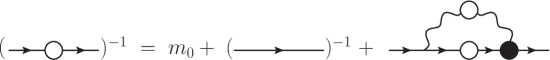
Figure 8: The SDE (gap equation) for the quark propagator, given by Eq. (23). The white blobs represent the fully dressed gluon and quark propagators, while the black blob denotes the dressed quark-gluon vertex.

The SDE for the quark propagator is shown diagrammatically in Fig. 8, and is given by

$$S^{-1}(p)=/{p}-m_{0}-C_{\rm F}g^{2}\int_{k}\Gamma_{\mu}^{[0]}S(k)\Gamma_{\nu}(-p,k,q)\Delta^{\mu\nu}(q)\,,$$ (23)

where $q\equiv p-k$, $\Gamma_{\nu}(-p,k,q)$ is the fully dressed quark-gluon vertex, $\Gamma_{\mu}^{[0]}$ is the tree-level value, and $C_{\rm F}$ is the Casimir eigenvalue in the fundamental representation. In this talk we will only consider the case of vanishing current quark mass, $m_{0}=0$, i.e., the chiral symmetry is kept intact at the Lagrangian level. One of the characteristic features of this integral equation is that, in order to give rise to nontrivial solutions, the support of its kernel in a special momentum regime must overcome a critical amount.

As happens in the case of the ghost equation, the nonperturbative vertex constitutes a crucial ingredient for overcoming the aforementioned critical amount and arriving to a physically acceptable solution. The situation, however, is much more complicated now, given that the tensorial decomposition of $\Gamma_{\nu}(-p,k,q)$ consists of twelve independent structures [72] instead of only two. Projecting them out of the SDE that governs $\Gamma_{\nu}(-p,k,q)$ represents a major technical challenge, let alone solving the resulting intricate system of coupled integral equations. Lattice simulations, on the other had, have obtained some of the corresponding form factors for special kinematic configurations [68, 69, 70], but their relevance to the problem at hand is relatively limited.

The alternative that has been extensively adopted is to employ gauge-technique inspired Ansätze (see, e.g.,  [71] and references therein) for $\Gamma_{\nu}(-p,k,q)$, namely construct it in such a way that it satisfies the STI imposed by the BRST symmetry. In particular, $\Gamma_{\mu}(p_{1},p_{2},p_{3})$ obeys the fundamental STI [2]

$$p_{3}^{\mu}\Gamma_{\mu}(p_{1},p_{2},p_{3})=F(p_{3})[S^{-1}(-p_{1})H(p_{1},p_{2},p_{3})-{\overline{H}}(p_{2},p_{1},p_{3})S^{-1}(p_{2})]\,,$$ (24)

where the fermion-ghost scattering kernel $H(p_{1},p_{2},p_{3})$ is defined diagrammatically in  Fig. 9, and has the tensorial decomposition

$$H(p_{1},p_{2},p_{3})=X_{0}\mathbb{I}+X_{1}/{p_{1}}+X_{2}/{p_{2}}+X_{3}\tilde{\sigma}_{\mu\nu}p_{1}^{\mu}p_{2}^{\nu},$$ (25)

with $\tilde{\sigma}_{\mu\nu}\equiv\frac{1}{2}[\gamma_{\mu},\gamma_{\nu}]$; ${\overline{H}}(p_{2},p_{1},p_{3})$ is the “conjugated” version of $H(p_{1},p_{2},p_{3})$ [72].

Note that when both $F$ and $H$ are set to unity (i.e., the ghost sector is switched off), Eq. (24) reduces to the text-book WI relating the photon-electron vertex with the electron propagator in QED. The the so-called Ball-Chiu (BC) vertex [73],

$$\Gamma^{\mu}_{\rm BC}(p_{1},p_{2},p_{3}) = \frac{A(p_{1})+A(p_{2})}{2}\gamma^{\mu}$$ (26)

$$+ \frac{(p_{1}-p_{2})^{\mu}}{p_{1}^{2}-p_{2}^{2}}\left\{\left[A(p_{1})-A(p_{2})\right]\frac{/{p_{1}}-/{p_{2}}}{2}+\left[B(p_{1})-B(p_{2})\right]\right\}\,.$$

satisfies precisely this particular WI, instead of the full STI of Eq. (24), and has served as the starting point of numerous studies.

Specifically, use of Eq. (26) into Eq. (23) leads to a coupled system for $A(p^{2})$ and $B(p^{2})$

$$A(p^{2}) = 1+C_{F}g^{2}\,\int_{k}\,\frac{{\cal K}(p-k)}{A^{2}(k^{2})k^{2}+B^{2}(k^{2})}{\cal K}_{A}^{\rm BC}(k,p)\,,$$

$$B(p^{2}) = C_{F}g^{2}\int_{k}\,\frac{{\cal K}(p-k)}{A^{2}(k^{2})k^{2}+B^{2}(k^{2})}{\cal K}_{B}^{\rm BC}(k,p)\,,$$ (27)

where the kernel ${\cal K}_{B}^{\rm BC}(k,p)$ originates from Eq. (26) (for its explicit form, see, e.g.,  [74]), while the kernel ${\cal K}(q)$ encompasses all remaining contributions.

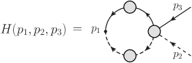
Figure 9: Diagrammatic representation of the ghost-gluon kernel $H$.

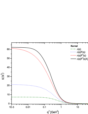
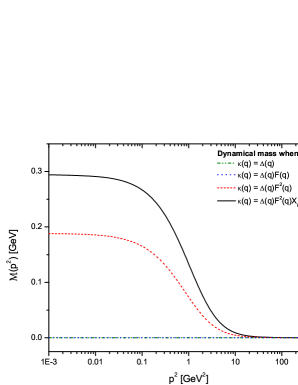
Figure 10: Left panel: The individual contribution of the ingredients composing ${\cal K}(q)$. The green dotted-dashed line represents the case where ${\cal K}(q)=\Delta(q)$, the blue dotted line the case where ${\cal K}(q)=\Delta(q)F(q)$, in the red dashed curve ${\cal K}(q)=\Delta(q)F^{2}(q)$ and, finally the black continuous line represents the case where ${\cal K}(q)$ assumes the full form used, namely ${\cal K}(q)=\Delta(q)F^{2}(q)X_{0}^{[1]}(q)$. Right panel: The corresponding dynamical quark mass generated when we use in Eq. (27) the different forms of ${\cal K}(q)$ shown in the left panel.

If the ghost contributions to $\Gamma_{\mu}$ are switched off, ${\cal K}(q)$ consists simply of $\Delta(q)$; in this case, however, the resulting combined kernel (right panel of Fig. 10) fails to furnish a nontrivial solution (left panel of Fig. 10).

Given this unsatisfactory situation, a next possible improvement consists in restoring the omitted ghost-related contributions to $\Gamma_{\mu}$, thus achieving the gradual “non-Abelianization” of the Ball-Chiu vertex. In particular, one may include the contributions of $F(q)$ and $H$, as dictated by the STI of Eq. (24). Evidently, since $F(q)$ is very well known (see previous section), the main challenge is to obtain an approximation for $H$, or at least, for some of its form factors. In addition, renormalization introduces (effectively) into ${\cal K}(q)$ an additional multiplicative factor of $F(q)$, an approximation which guarantees that the anomalous dimension of the resulting dynamical quark mass is consistent with the known one-loop expression (see also [75]). On the right panel of Fig. 10 one may follow the gradual built-up of ${\cal K}(q)$ and on the left the form of the quark mass $\mathcal{M}(p^{2})$ obtained at each step. Evidently, when ${\cal K}(q)=F^{2}(q)\Delta(q)$, a considerable amount of $\mathcal{M}(p^{2})$ is obtained from Eq. (27); however, one deviates by a factor of about $30\%$ from the phenomenologically accepted value.

It turns out that the missing amount of dynamical quark mass may be obtained by supplying to ${\cal K}(q)$ some of the strength coming from $H$. In particular, the form factor $X_{0}$ was computed within the one-loop dressed approximation, $X_{0}^{[1]}$, for the symmetric kinematic configuration $(-q/2,-q/2,q)$ [74]. The result is shown in Fig. 11; note that the deviation from unity (peaked around 600 MeV) is modest, but, due to the nonlinearity of the gap equation, it gives rise to a considerable amount of additional quark mass, as can be appreciated in Fig. 10.

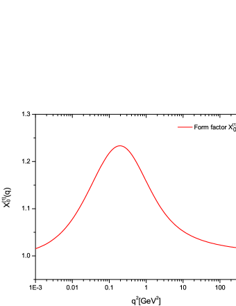
Figure 11: Numerical result for the form factor $X_{0}^{[1]}(q)$, obtained within the one-loop dressed approximation, using fully dressed propagators and bare vertices [74].

6 Hadron observables from continuum QCD

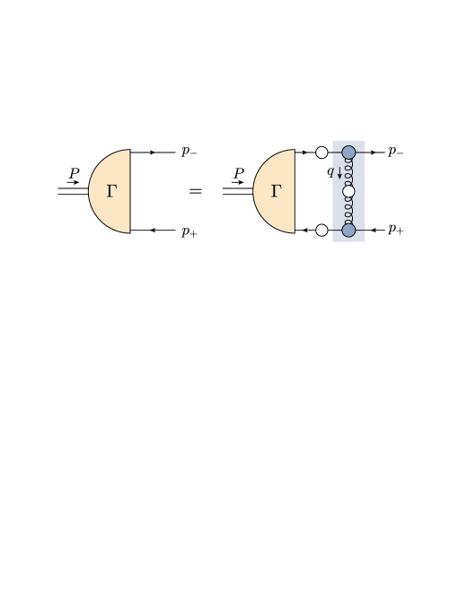
Figure 12: A typical Bethe-Salpeter equation. The blue box contains the interaction kernel, whose form is crucial for the type of solutions (spectrum) obtained.

One of the longstanding challenges of QCD is to furnish quantitatively accurate ab initio predictions for the observable properties of hadrons [76, 77, 78, 79]. In a recent work [80], considerable progress has been made in this direction; in what follows we will highlight the main aspects of these new developments.

Let us consider the kernel appearing in a typical Bethe-Salpeter equation [81], shown in Fig. 12, which is contained in the blue box. This kernel receives a “universal” (process-independent) contribution, whose origin is the pure gauge sector of the theory. In that sense, this contribution constitutes the common ingredient of any such kernel, regardless of the nature of the particles between which it is embedded; most notably, it does not depend on the valence-quark content of the Bethe-Salpeter equation.

The systematic diagrammatic identification of the precise pieces that constitute this particular quantity may be carried out following the PT. As has been explained in detail in the literature, the upshot of this construction is the rearrangement of a physical amplitude into sub-amplitudes with very special properties [7]. In addition, it is well-known that the result of this particular rearrangement coincides with the $BB$ gluon propagator defined in the BFM (see [6] and references therein).

Specifically, the standard $\Delta(q^{2})$ introduced in Eq. (1) and the corresponding quantity of the $BB$ gluon propagator, denoted by $\widehat{\Delta}(q^{2})$, are related by the exact relation

$$\Delta(q^{2})=\widehat{\Delta}(q^{2})[1+G(q^{2})]^{2}\,,$$ (28)

which is completely analogous to Eq. (8).

At the one-loop level, and keeping only ultraviolet logarithms, one has [39]

$$1+G(q^{2}) = 1+\left(\frac{9}{4}\right)\frac{\alpha_{s}C_{\rm{A}}}{12\pi}\ln\left(\frac{q^{2}}{\mu^{2}}\right),$$

$$\Delta^{-1}(q^{2}) = q^{2}\left[1+\left(\frac{13}{2}\right)\frac{\alpha_{s}C_{\rm{A}}}{12\pi}\ln\left(\frac{q^{2}}{\mu^{2}}\right)\right]^{-1},$$ (29)

and thus

$$\widehat{\Delta}^{-1}(q^{2})=q^{2}\left[1+b\alpha_{s}\ \ln\left(\frac{q^{2}}{\mu^{2}}\right)\right].$$ (30)

where $b=11C_{A}/12\pi$ is the first coefficient of the Yang-Mills $\beta$ function, as it should [8].

Due to the special WIs satisfied by the PT-BFM Green’s functions, the (dimensionful) universal combination

$${\widehat{d}}(q^{2})=\alpha_{s}\widehat{\Delta}(q^{2})=\frac{\alpha_{s}\Delta(q^{2})}{\left[1+G(q^{2})\right]^{2}}$$ (31)

is renormalization-group invariant. In particular, the renormalization constants of the gauge-coupling and of $\widehat{\Delta}^{-1}(p^{2})$, defined as

$$g(\mu^{2}) = Z_{g}^{-1}(\mu^{2})g_{0},$$

$$\widehat{\Delta}(p^{2},\mu^{2}) = \widehat{Z}^{-1}_{A}(\mu^{2})\widehat{\Delta}_{0}(p^{2}),$$ (32)

where the “0” subscript indicates bare quantities, satisfy the QED-like relation

$${Z}_{g}={\widehat{Z}}^{-1/2}_{A}.$$ (33)

Therefore,

$${\widehat{d}}_{0}(q^{2})={\alpha_{s}}_{0}\widehat{\Delta}_{0}(q^{2})=\alpha_{s}(\mu^{2})\widehat{\Delta}(q^{2},\mu^{2})={\widehat{d}}(q^{2})$$ (34)

maintains the same form before and after renormalization, i.e., it forms a $\mu$-independent quantity.

This last property has been explicitly verified to an impressive accuracy, following the procedure summarized in Fig. 13 and Fig. 14. The gluon propagator $\Delta(q^{2})$, obtained from the lattice data of [31], is multiplicatively renormalized (in the momentum-subtraction scheme) at five different values of $\mu$. The dynamical equation furnishing $1+G(q^{2})$ (not reported here, see [82, 83]) is subsequently solved, for the same values of $\mu$. When the resulting curves (given in the two panels of Fig. 13) are combined according to Eq. (31), it turns out that a unique curve emerges, provided that the values of each $\alpha_{s}(\mu^{2})$ are those shown in the insert of  Fig. 14.

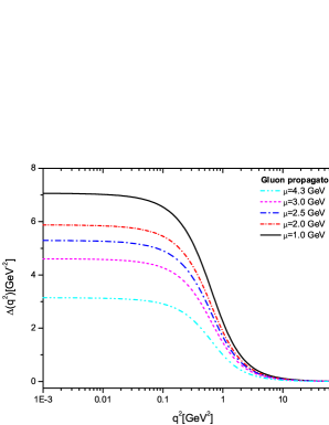
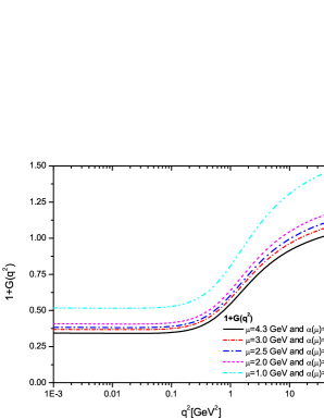
Figure 13: Left panel:: The gluon propagator for different values of the renormalization point $\mu$. Right panel: The auxiliary function $1+G(q^{2})$ for the same set of values of $\mu$.

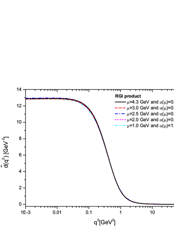
Figure 14: The RG-invariant product ${\widehat{d}}(q^{2})$ put together according Eq. (31), using the results of Fig. 13: one practically obtains one single curve for all different values of the renormalization point $\mu$

From the dimensionful quantity ${\widehat{d}}(q^{2})$ one may extract a dimensionless effective charge, to be denoted by ${\cal I}(q^{2})$, by simply pulling out a factor of $q^{2}$, namely

$${\cal I}(q^{2})=q^{2}{\widehat{d}}(q^{2})\,.$$ (35)

This SDE-derived quantity allows for a direct comparison with an analogous quantity commonly employed by practitioners for describing the (momentum-dependent) interaction between quarks, obtained through a well-defined truncation of the equations in the matter sector that are relevant to bound-state properties. In particular, one uses

$${\cal I}(q^{2})=k^{2}{\cal G}(q^{2});\quad{\cal G}(q^{2})=\frac{8\pi^{2}}{\omega^{4}}D{\mathrm{e}}^{-q^{2}/\omega^{2}}+\frac{8\pi^{2}\gamma_{m}(1-{\mathrm{e}}^{-q^{2}/4m_{t}^{2}})}{q^{2}\ln[\tau+(1+q^{2}/\Lambda_{\scriptscriptstyle\rm QCD}^{2})^{2}]},$$ (36)

where $\gamma_{m}=12/(33-2N_{f})$ [typically, $N_{f}=4$], $\Lambda_{\scriptscriptstyle\rm QCD}=0.234$ GeV; $\tau={\rm e}^{2}-1$, $m_{t}=0.5$ GeV. A large body of observable properties of ground-state vector- and isospin-nonzero pseudoscalar mesons (and even numerous properties of the nucleon and $\Delta$ resonance) are practically insensitive to variations of $\omega\in[0.4,0.6]$ GeV, so long as $\varsigma^{3}=D\omega=$const. The value of $\varsigma$ is typically chosen to obtain the measured value of $f_{\pi}$; however its value depend on the truncation scheme used when deriving (36). The usual rainbow-ladder (RL) truncation [84] yields $\varsigma_{\scriptscriptstyle\rm RL}=0.87$ GeV, while the improved truncation scheme (DB) of [76] gives $\varsigma_{\scriptscriptstyle\rm DB}=0.55$ GeV.

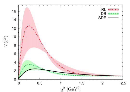
Figure 15: Comparison between the SDE-derived effective interaction obtained from the gauge-sector [Eq. (35), solid, black] with those obtained using Eq. (36): pale-red band: RL truncation, pale-green band: DB truncation. The bands denote the domain of constant ground-state physics $0.45<\omega<0.6$, with the curve within each band obtained with $\omega=0.5\,$GeV.

As can be seen in Fig. 15, the direct comparison between the ${\cal I}(q^{2})$ defined through Eq. (35) and Eq. (36) reveals an excellent agreement. This seems to suggest that a QCD-derived description of measurable hadron properties is well within our reach.

7 Conclusions

In this presentation we have reviewed a large body of developments related to the study of the off-shell Green’s functions of pure Yang-Mills theories and QCD, using SDEs and the lattice simulations in the Landau gauge. The general picture that surfaces may be summarized as follows:

i) Gluons just as quarks acquire a dynamical mass, which is controlled by the corresponding “gap equation”.

ii) Ghosts remain massless, and have a finite dressing function that can be accurately obtained from the corresponding SDE.

iii) The quality of the ingredients entering into the quark gap equation is steadily improving, giving rise to phenomenologically successful quark masses.

iv) A significant step has been taken for bridging the gap between nonperturbative continuum QCD predictions and hadron phenomenology.

Even though a lot of work remains to be done in all directions, Richard Feynman’s famous quote from the first of his seven “Messenger Lectures” at Cornell University in 1964 comes to mind: Nature uses only the longest threads to weave her patterns, so that every small piece of the fabric reveals the organization of the entire tapestry”. We seem to have reached a similar point with QCD: even though the Green’s functions that have been studied are but a small piece of the QCD fabric, unequivocal signs of an underlying organization begin to emerge.

This research is supported by the Spanish MEYC under grant FPA2011-23596 and the Generalitat Valenciana under grant “PrometeoII/2014/066”. I would like to thank the organizers of the “Discrete 2014” for their kind invitation and hospitality, and all participants for providing a most stimulating and pleasant atmosphere.

References

References

- [1] C. N. Yang and R. L. Mills, Phys. Rev. 96, 191 (1954).
- [2] W. J. Marciano and H. Pagels, Phys. Rept. 36, 137 (1978).
- [3] J. M. Cornwall, Phys. Rev. D 26, 1453 (1982).
- [4] J. M. Cornwall and J. Papavassiliou, Phys. Rev. D 40, 3474 (1989).
- [5] A. Pilaftsis, Nucl. Phys. B 487, 467 (1997).
- [6] D. Binosi and J. Papavassiliou, Phys. Rev. D 66, 111901 (2002).
- [7] D. Binosi and J. Papavassiliou, Phys. Rept. 479, 1 (2009).
- [8] L. F. Abbott, Nucl. Phys. B 185, 189 (1981).
- [9] R. Alkofer and L. von Smekal, Phys. Rept. 353, 281 (2001).
- [10] A. C. Aguilar and A. A. Natale, JHEP 0408, 057 (2004).
- [11] C. S. Fischer, J. Phys. G 32, R253 (2006).
- [12] J. Braun, H. Gies and J. M. Pawlowski, Phys. Lett. B 684, 262 (2010).
- [13] P. Boucaud, J. P. Leroy, A. L. Yaouanc, J. Micheli, O. Pene and J. Rodriguez-Quintero, JHEP 0806, 012 (2008).
- [14] P. Boucaud, J. P. Leroy, A. Le Yaouanc, J. Micheli, O. Pene and J. Rodriguez-Quintero, JHEP 0806, 099 (2008).
- [15] D. Dudal, J. A. Gracey, S. P. Sorella, N. Vandersickel and H. Verschelde, Phys. Rev. D 78, 065047 (2008).
- [16] C. S. Fischer, A. Maas and J. M. Pawlowski, Annals Phys. 324, 2408 (2009).
- [17] M. R. Pennington and D. J. Wilson, Phys. Rev. D 84, 119901 (2011).
- [18] J. Serreau and M. Tissier, Phys. Lett. B 712, 97 (2012).
- [19] M. Tissier and N. Wschebor, Phys. Rev. D 84, 045018 (2011).
- [20] F. Siringo, Phys. Rev. D 90, no. 9, 094021 (2014).
- [21] C. D. Roberts and A. G. Williams, Prog. Part. Nucl. Phys. 33, 477 (1994).
- [22] P. Maris and C. D. Roberts, Int. J. Mod. Phys. E 12, 297 (2003).
- [23] A. C. Aguilar and J. Papavassiliou, JHEP 0612, 012 (2006).
- [24] P. A. Grassi, T. Hurth and M. Steinhauser, Annals Phys. 288, 197 (2001).
- [25] D. Binosi and J. Papavassiliou, Phys. Rev. D 66, 025024 (2002).
- [26] D. Binosi and J. Papavassiliou, Phys. Rev. D 77, 061702 (2008).
- [27] D. Binosi and J. Papavassiliou, JHEP 0811, 063 (2008).
- [28] C. W. Bernard, Nucl. Phys. B 219, 341 (1983).
- [29] J. F. Donoghue, Phys. Rev. D 29, 2559 (1984).
- [30] I. L. Bogolubsky, E. M. Ilgenfritz, M. Muller-Preussker and A. Sternbeck, Phys. Lett. B 676, 69 (2009).
- [31] I. L. Bogolubsky, E. M. Ilgenfritz, M. Muller-Preussker and A. Sternbeck, PoS LAT 2007, 290 (2007).
- [32] P. O. Bowman, U. M. Heller, D. B. Leinweber, M. B. Parappilly, A. Sternbeck, L. von Smekal, A. G. Williams and J. b. Zhang, Phys. Rev. D 76, 094505 (2007).
- [33] O. Oliveira and P. J. Silva, PoS LAT 2009, 226 (2009).
- [34] A. Cucchieri and T. Mendes, PoS LAT 2007, 297 (2007).
- [35] A. Cucchieri and T. Mendes, Phys. Rev. Lett. 100, 241601 (2008).
- [36] A. Cucchieri and T. Mendes, Phys. Rev. D 81, 016005 (2010).
- [37] A. Cucchieri and T. Mendes, PoS QCD -TNT09, 026 (2009).
- [38] O. Philipsen, Nucl. Phys. B 628, 167 (2002).
- [39] A. C. Aguilar, D. Binosi and J. Papavassiliou, Phys. Rev. D 78, 025010 (2008).
- [40] J. S. Schwinger, Phys. Rev. 125, 397 (1962).
- [41] J. S. Schwinger, Phys. Rev. 128, 2425 (1962).
- [42] R. Jackiw and K. Johnson, Phys. Rev. D 8, 2386 (1973).
- [43] R. Jackiw, In *Erice 1973, Proceedings, Laws Of Hadronic Matter*, New York 1975, 225-251 and M I T Cambridge - COO-3069-190 (73,REC.AUG 74) 23p
- [44] J. M. Cornwall and R. E. Norton, Phys. Rev. D 8, 3338 (1973).
- [45] E. Eichten and F. Feinberg, Phys. Rev. D 10, 3254 (1974).
- [46] E. C. Poggio, E. Tomboulis and S.-H. H. Tye, Phys. Rev. D 11, 2839 (1975).
- [47] A. C. Aguilar, D. Ibanez, V. Mathieu and J. Papavassiliou, Phys. Rev. D 85, 014018 (2012).
- [48] D. Ibanez and J. Papavassiliou, Phys. Rev. D 87, no. 3, 034008 (2013)
- [49] A. C. Aguilar and J. Papavassiliou, Phys. Rev. D 81, 034003 (2010).
- [50] D. Binosi, D. Ibanez and J. Papavassiliou, Phys. Rev. D 86, 085033 (2012).
- [51] A. C. Aguilar, D. Binosi and J. Papavassiliou, Phys. Rev. D 89, no. 8, 085032 (2014).
- [52] This demonstration is taken from Peter C. Tandy’s talk “Some Chapters from the Do-It-Yourself Hadron Theory Manual”.
- [53] I. C. Cloet and C. D. Roberts, Prog. Part. Nucl. Phys. 77, 1 (2014).
- [54] L. Del Debbio, M. Faber, J. Greensite and S. Olejnik, Phys. Rev. D 55 (1997) 2298.
- [55] A. P. Szczepaniak and E. S. Swanson, Phys. Rev. D 65, 025012 (2002).
- [56] K. Langfeld, H. Reinhardt and J. Gattnar, Nucl. Phys. B 621, 131 (2002).
- [57] A. P. Szczepaniak, Phys. Rev. D 69, 074031 (2004).
- [58] J. Greensite, Prog. Part. Nucl. Phys. 51, 1 (2003).
- [59] J. Gattnar, K. Langfeld and H. Reinhardt, Phys. Rev. Lett. 93, 061601 (2004).
- [60] J. Greensite, H. Matevosyan, S. Olejnik, M. Quandt, H. Reinhardt and A. P. Szczepaniak, Phys. Rev. D 83, 114509 (2011).
- [61] A. Cucchieri, T. Mendes and A. Mihara, JHEP 0412, 012 (2004).
- [62] A. Cucchieri, A. Maas and T. Mendes, Phys. Rev. D 74, 014503 (2006).
- [63] A. Cucchieri, A. Maas and T. Mendes, Phys. Rev. D 77, 094510 (2008).
- [64] A. C. Aguilar, D. Ibanez and J. Papavassiliou, Phys. Rev. D 87, no. 11, 114020 (2013).
- [65] D. Dudal, O. Oliveira and J. Rodriguez-Quintero, Phys. Rev. D 86, 105005 (2012).
- [66] P. Boucaud, F. de Soto, J. P. Leroy, A. Le Yaouanc, J. Micheli, H. Moutarde, O. Pene and J. Rodriguez-Quintero, Phys. Rev. D 74, 034505 (2006).
- [67] P. Boucaud, F. De Soto, J. P. Leroy, A. Le Yaouanc, J. Micheli, O. Pene and J. Rodriguez-Quintero, Phys. Rev. D 79, 014508 (2009).
- [68] J. Skullerud and A. Kizilersu, JHEP 0209, 013 (2002).
- [69] J. I. Skullerud, P. O. Bowman, A. Kizilersu, D. B. Leinweber and A. G. Williams, JHEP 0304, 047 (2003).
- [70] A. Kizilersu, D. B. Leinweber, J. I. Skullerud and A. G. Williams, Eur. Phys. J. C 50, 871 (2007).
- [71] A. Kizilersu and M. R. Pennington, Phys. Rev. D 79, 125020 (2009).
- [72] A. I. Davydychev, P. Osland and L. Saks, Phys. Rev. D 63, 014022 (2001).
- [73] J. S. Ball and T. W. Chiu, Phys. Rev. D 22, 2542 (1980).
- [74] A. C. Aguilar and J. Papavassiliou, Phys. Rev. D 83, 014013 (2011).
- [75] C. S. Fischer and R. Alkofer, Phys. Rev. D 67, 094020 (2003).
- [76] L. Chang and C. D. Roberts, Phys. Rev. Lett. 103, 081601 (2009).
- [77] L. Chang, Y. X. Liu and C. D. Roberts, Phys. Rev. Lett. 106, 072001 (2011).
- [78] S. x. Qin, L. Chang, Y. x. Liu, C. D. Roberts and D. J. Wilson, Phys. Rev. C 85, 035202 (2012).
- [79] L. Chang and C. D. Roberts, Phys. Rev. C 85, 052201 (2012).
- [80] D. Binosi, L. Chang, J. Papavassiliou and C. D. Roberts, Phys. Lett. B 742, 183 (2015).
- [81] G. Eichmann, arXiv:0909.0703 [hep-ph].
- [82] A. C. Aguilar, D. Binosi and J. Papavassiliou, JHEP 0911, 066 (2009).
- [83] A. C. Aguilar, D. Binosi, J. Papavassiliou and J. Rodriguez-Quintero, Phys. Rev. D 80, 085018 (2009).
- [84] P. Maris and P. C. Tandy, Phys. Rev. C 60, 055214 (1999).