A Modest Revision of the Standard Model

Abstract

With a modest revision of the Standard Model, in the fermion mass sector only, the systematics of the fermion masses and mixings can be fully described and interpreted as providing information on matrix elements of physics beyond the Standard Model. A by-product is a reduction of the largest Higgs Yukawa fine structure constant by an order of magnitude. The extension to leptons provides for insight on the difference between quark mixing and lepton mixing as evidenced in neutrino oscillations. The substantial difference between the scale for up-quark and down-quark masses is not addressed. In this approach, improved detail and accuracy of the elements of the current mixing matrices can extend our knowledge and understanding of physics beyond the Standard Model.

I Introduction

For several decades, the quantum numbers and corresponding gauge interactions that distinguish the different generations of fermions have been sought without overt success. The various efforts to understand the fermion masses have ranged from substructure to Grand Unification. The former approaches include rishonsHarari and technicolorHoldom , but always encounter a fundamental problem: For relativistic constituents, the limiting gaps between eigenstates tend to a constant value, as in the MIT bag modelKiskis (surprisingly parallel to the eigen structure for the non-relativistic harmonic oscillator). With sufficiently strange potentials (e.g., the “dracula” potentialKostelecky ), the lowest few states may be forced to match the increasing gaps found in the real world, but they ultimately tend to a constant gap and predict additional states within the range of experiment that remain unseen. The latter approach has found some interesting relations between quarks and leptonsGeorgi-Glashow ; seesaw and even some mixing anglesFritzsch but no convincing overall solution has been obtained. Efforts along these lines have continued.recentarXiv

We consider a revision of the Standard Model (SM), in the fermion mass sector only, by taking a contrary point of view, namely that, within the (revised) SM, all of the fermions with a given electric charge should be viewed as having nothing that makes their right-chiral, weak interaction singlet components distinguishable to the Higgs boson. That is, we take the Higgs coupling to be completely insensitive to “generation” and discard the Yukawa coefficients that have been (artificially) inserted in the SM to reproduce the observed masses.

In the past, many others have constructed similar mass matrices by starting from various symmetry assumptions. A few of them, of which we are aware, are referenced here. others ; Jarl They are all “top-down” approaches, making initial symmetry assumptions. Conversely, we take a “bottom-up” starting point focusing on the absence of a known symmetry or quantum numbers. This may be viewed as an accidental $S_{3}$ symmetry but that is not the fundamental nature of our basic assumption. Rather, we assume that the final form of the fermion mass matrix is determined by all possible (loop) corrections to the SM from physics beyond the SM (BSM physics) and invert the relation to extract information on some matrix elements of BSM physics. This should be contrasted especially with the approach in previous work, such as for example in Refs.(referee ), where the number of unknown BSM parameters is reduced by assuming only limited forms for the initial mass matrices.

We apply this concept here to the quarks and comment on related implications for leptons, reserving a full discussion of the leptonic system, including neutrinos and their additional complications, to a later paper. This approach amounts to a small change in the mass sector of the SM, (hence, a modest revision, albeit a “massive” one) which provides an interpretation, in terms of BSM physics, of the deviations from the direct mass implications of our revised version of the SM.

We obtain a consistent description of the quark masses and weak interaction current mixing for BSM corrections on the order of 1%, and constrain relations among the (many) allowed BSM parameters, with values that are “natural” in the classic sense ($O(1)$). We find that non-Cartan sub-algebra components of the BSM symmetry-breaking corrections are required.

Although this approach proposes a resolution of the differences in fermion masses between “generations”, it does not attempt to address the differences in mass scale between the fermions of different electric charge, generally described as within “families”. Our approach does, however, reduce the number of these questions to two for the quarks and provides for a similar reduction for the leptons.

I.1 Mass in the SM

We first briefly review the structure of SM mass terms that we will revise. They are set by (arbitrary) Yukawa couplings of the (one, or in supersymmetry, at least two) Higgs boson(s) to the weak interaction active left-chiral doublets and weak interaction “sterile” (except for their $U(1)_{B}$ quantum numbers) singlets. The form is

$${\cal L}_{m}= \Sigma_{i}Y_{Ui}\overline{\left(\frac{1+\gamma_{5}}{2}\right)\Psi_{Ui}}<\phi^{0},\phi^{+}>\left(\frac{1-\gamma_{5}}{2}\right)\left[\begin{array}[]{c}\Psi_{Ui}\\ \Psi_{Di}\end{array}\right]+h.c.$$ (3)

$$+ \Sigma_{i}Y_{Di}\overline{\left(\frac{1+\gamma_{5}}{2}\right)\Psi_{Di}}<\phi^{-},\phi^{0*}>\left(\frac{1-\gamma_{5}}{2}\right)\left[\begin{array}[]{c}\Psi_{Ui}\\ \Psi_{Di}\end{array}\right]+h.c.$$ (6)

where the Higgs may be the same or different in the two sets of terms.

Unlike the comparable terms for the interaction with the weak gauge bosons, which is naturally in the current basis, this Dirac notation is in the mass eigenstate basis and suppresses the information that pairs of independent Weyl spinors are involved. In the SM, the $Y_{i}$ are taken to equal the mass of the appropriate fermion divided by the vacuum expectation value of the Higgs boson.

In a more general notation, a Dirac bispinor is composed of two Weyl spinors vile

$$\Psi=\left[\begin{array}[]{c}\xi\\ \chi\end{array}\right]$$ (7)

where these two chiral spinors are constructed from another pair ($\zeta_{a}$ and $\zeta_{b}$) with a fixed phase relation, as

$$\xi = \zeta_{a}+\zeta_{b}$$ (8)

$$\chi = \sigma_{2}(-\zeta^{*}_{a}+\zeta^{*}_{b})$$ (9)

so that the Dirac mass term appears as

$$\overline{\Psi}\Psi=-(\chi^{\dagger}\xi+\xi^{\dagger}\chi).$$ (10)

This makes it clear that the Dirac mass term couples two independent Weyl spinors (left- and right-chiral) one of which is weak interaction active and the other sterile as described above.

For completeness, we display the Majorana form for a Weyl spinor and its mass term:

$$\Psi_{M}=\left[\begin{array}[]{c}\xi\\ -\sigma_{2}\xi^{*}\end{array}\right]\;,\;\;\overline{\Psi_{M}}\Psi_{M}=-(\xi^{\dagger}\sigma_{2}\xi^{*}+\xi^{T}\sigma_{2}\xi)$$ (11)

which will be relevant when we refer to neutrinos later.

I.2 Basic concept

The weak iso-singlet produced by the coupling of the Higgs boson to the left-chiral projection of the quark (generally, fermion) doublet has no known quantum number besides that of the U(1) that completes the electric charges of the fields. Similarly, the right-chiral projections have no known other quantum number. Hence we are free to choose bases in the left- and right-chiral representation spaces such that the entries to the mass matrix for all of the quark (fermion) fields of a given charge are identical. The corresponding mass matrix appears to have been first described as “democratic” by Jarlskog Jarl , although, for larger dimensional forms, it is known in nuclear and condensed matter physics as the origin of the “pairing gap”. The eigenstates for such a system consist of one (non-zero energy or) massive state with all other (two in the case of interest here) eigenstates being (at zero energy or) massless. This provides for a natural starting point consistent with the large gap between the heaviest and the lighter known fundamental fermions (of each charged type). We address the question of basis choice below in Sec.III.

Experimentally, however, the lighter fermions in each grouping are not massless. This deviation from zero mass for the lighter fermions can be accommodated by assuming small deviations from “democracy”, consistent with perturbative corrections from BSM physics, which quite naturally allows for small mass eigenstates in the final result. A particular constraint on the parameters of the BSM physics is required for one of these to be much smaller than the other. Under our assumption, these effects afford a glimpse into the nature and structure of the BSM physics by requiring specific relationships between some matrix elements (that would be calculable from any given BSM theory).

The constraints can be discerned by examining the matrix, $U$, that relates the BSM-corrected mass eigenstates to the weak interaction eigenstates, for the up-quarks, and the corresponding matrix, $V$, for the down-quarks, combined into the form $UV^{\dagger}$ that produces the Cabibbo-Kobayashi-Maskawa Cab ; KM (CKM) matrix in the form as described by the Particle Data Group PDG (PDG). That is, our approach recognizes that the Higgs coupling to the “active”, left-chiral, weak iso-doublet fermions is aligned with the weak gauge boson coupling, and so is diagonal in that (Weyl spinor) basis. As stated above, however, we take as a given that the right-chiral, weak iso-singlet Weyl spinors all present themselves indistinguishably to the weak iso-singlet object formed by combining the Higgs doublet with the active fermion doublet. The CKM matrix is produced conventionally by the misalignment between the mass and weak eigenstates, but here determined from the two separate components, $U$ and $V^{\dagger}$.

Another feature of the mass eigenstates of the $3\times 3$ “democratic” matrix is that the eigenvectors for the mass eigenstates can take the form of a tri-bi-maximal (TBM) mixture of the original (current) eigenstates. One state must be maximally mixed; for the other two, one has a degeneracy choice. However, there is no impediment to an overall TBM choice. While useful to simplify calculations, this is not particularly significant for the quarks, as the TBM structure cancels out in construction of the CKM matrix. (See Eqs.(99,100) below.) However, it does have significant implications for the difference between the CKM and the corresponding Pontecorvo-Maki-Nakagawa-Sakata PMNS (PMNS) matrix for mixing in the lepton sector. We will comment upon this difference in our conclusions.

II Starting point and positive indications

The tri-bi-maximal (TBM) matrix

$$TBM=\left[\begin{array}[]{ccc}\frac{1}{\sqrt{6}}&-\frac{1}{\sqrt{2}}&\frac{1}{\sqrt{3}}\\ \frac{1}{\sqrt{6}}&\frac{1}{\sqrt{2}}&\frac{1}{\sqrt{3}}\\ -\frac{2}{\sqrt{6}}&0&\frac{1}{\sqrt{3}}\\ \end{array}\right]$$ (12)

diagonalizes the “democratic” matrix

$$M_{dem}=\frac{1}{3}\times\left[\begin{array}[]{ccc}1&1&1\\ 1&1&1\\ 1&1&1\\ \end{array}\right]$$ (13)

to

$$M_{m} = TBM^{\dagger}\times M_{dem}\times TBM$$ (17)

$$= \left[\begin{array}[]{ccc}0&0&0\\ 0&0&0\\ 0&0&1\\ \end{array}\right]$$

where we have chosen the overall scale so the nonzero eigenvalue is unity.

The efficacy of the “democratic” conjecture can be tested by inverting the TBM transformation on the known quark masses (taken from the PDGPDG and) placed into diagonal mass matrices, viz.,

$$m_{u}=\left[\begin{array}[]{ccc}2.3&0&0\\ 0&1275&0\\ 0&0&173500\end{array}\right]\\$$ (18)

and

$$m_{d}=\left[\begin{array}[]{ccc}3.8&0&0\\ 0&95&0\\ 0&0&4150\end{array}\right]$$ (19)

where all values are expressed in MeV/$c^{2}$. (We will ignore the significant uncertainties and variation with scale of these massesscale as the ratios vary less dramatically, although the values of even the ratios are not known to very high accuracy.)

We now transform these inversely using the $TBM$ matrix given in Eq.(12) and find that the resulting mass matrices are indeed quite “democratic”:

$$m_{u-TBM} = TBM\times m_{u}\times TBM^{\dagger}$$ (23)

$$= (173500)\times\left[\begin{array}[]{ccc}0.33701&0.32966&0.33333\\ 0.32966&0.33701&0.33333\\ 0.33333&0.33333&0.33334\end{array}\right]$$

and similarly

$$m_{d-TBM}=(4150)\times\left[\begin{array}[]{ccc}0.34493&0.32204&0.33303\\ 0.32204&0.34493&0.33303\\ 0.33303&0.33303&0.33394\end{array}\right]$$ (24)

where we have scaled out the overall factor of the largest mass in each case. Although the true accuracy is, of course, far less, we keep the extra digits to display which matrix elements are not identical after the (inverse) TBM transformation and so convey the patterns that will survive even substantial (within experimental uncertainties) changes in the ratios of the diagonal values.

This demonstrates that only perturbatively small corrections to a democratic starting point are needed. (We have ignored $CP$-violation considerations here, but will return to them below.) The deviations from “democracy” are exceptionally small, less than 1% in the up-quark sector and less than 4% in the down-quark sector (for positive and negative deviations from an average). It is clear from this that something close in structure to $M_{dem}$ (times an overall mass scale, $m$) is a reasonable ansatz to consider for an initial mass matrix. (A similar result holds for the charged leptons.)

This result confirms that the wide range of quark masses is well described by an almost “democratic” mass matrix for each charge set of quarks, leaving only the overall scale difference between up-quarks and down-quarks (and also leptons) to be understood. We do not address that difference here.

III A Modestly Revised Mass Sector

With these comments and results in mind, we propose the mrSM (modestly revised Standard Model) which differs from the SM only in the fermion mass sector. In terms parallel to those of the SM used above, we have

$${\cal L}_{mr}= Y_{U}\Sigma_{i,j}\overline{\left(\frac{1+\gamma_{5}}{2}\right)\Psi_{Ui}}<\phi^{0},\phi^{+}>\left(\frac{1-\gamma_{5}}{2}\right)\left[\begin{array}[]{c}\Psi_{Uj}\\ \Psi_{Dj}\end{array}\right]+h.c.$$ (27)

$$+ Y_{D}\Sigma_{i,j}\overline{\left(\frac{1+\gamma_{5}}{2}\right)\Psi_{Di}}<\phi^{-},\phi^{0*}>\left(\frac{1-\gamma_{5}}{2}\right)\left[\begin{array}[]{c}\Psi_{Uj}\\ \Psi_{Dj}\end{array}\right]+h.c.$$ (30)

There is now only one $Y$ each for all of the up- and down-quarks and these two values are approximately one third of the value of the two largest $Y_{i}$ in the SM.

Of course, as long as each up-quark is related to a particular down-quark by the weak interaction, one may choose a “rotation” of the pair to any basis. We reiterate the basic points: Because there are no known quantum number restraints, we are free to rotate the bases for both the left- and right-chiral fields independently to ensure that the mass matrix is democratic. (With some particular BSM theory, this should be the basis required by quantum number constraints.) In that basis, it is clear that BSM corrections are perturbatively small, a situation in physics always much to be desired. This is especially so here, since effects of BSM physics, if they exist at all, must be suppressed.

We note, as lagniappe, that this factor of $3$ reduction in these remaining two Yukawa couplings to the Higgs field from the largest value in each case in the SM improves the formally perturbative character of this part of the SM by reducing the (set of) Higgs fine structure constant(s), $Y^{2}$/$4\pi$, by an order of magnitude. Of course, the total size of the effects of quark loops is unaltered, as the sum over all channels produces the same significant net effect as in the diagonal mass basis. However, the size of the total contribution becomes due to the number of diagrams contributing, not to any individual large one.

We take the full Higgs plus BSM-loop-corrected mass matrix to have the form

$${\mathcal{M}_{mrSM}}=m\times[{\mathcal{M}_{dem}}+\epsilon{\mathcal{M}_{BSM}}]$$ (31)

now in the current quark basis consistently defined by the Higgs and weak vector boson couplings. That is, we define the mass matrix for each set of 3 quarks of a given electric charge as $m$ (an overall scale which is approximately one-third of the mass of the most massive of each triple of the fermions of a given non-zero electric charge) times the matrix ${\mathcal{M}}$, where

$${\mathcal{M}} = \frac{(1+\epsilon\xi)}{3}\times\left[\begin{array}[]{ccc}1&1&1\\ 1&1&1\\ 1&1&1\\ \end{array}\right]$$ (35)

$$+ \epsilon\times\left[\begin{array}[]{ccc}\sqrt{\frac{2}{3}}y_{0}+y_{3}+\frac{1}{\sqrt{3}}y_{8}&y_{1}-I{y_{2}}&y_{4}-I{y_{5}}\\ y_{1}+I{y_{2}}&\sqrt{\frac{2}{3}}y_{0}-y_{3}+\frac{1}{\sqrt{3}}y_{8}&y_{6}-I{y_{7}}\\ y_{4}+I{y_{5}}&y_{6}+I{y_{7}}&\sqrt{\frac{2}{3}}y_{0}-\frac{2}{\sqrt{3}}y_{8}\\ \end{array}\right]$$ (39)

This allows for the most general set of perturbative (for small $\epsilon$) deviations possible for a Hermitean $3\times 3$ matrix from the democratic mass matrix produced by uniform Higgs’ coupling in each quark charge sector. The coefficients are chosen to match the normalization of the standard Gell-Mann $SU(3)$ ($U(3)$) basis matrices.

The BSM corrections are all taken to be proportional to the small quantity, $\epsilon$, defined by the diagonal matrix of known mass eigenvalues, (again, with the overall scale factored out)

$$m\times\left[\begin{array}[]{ccc}\epsilon\delta&0&0\\ 0&\epsilon&0\\ 0&0&1\\ \end{array}\right]$$ (40)

The overall factor $(1+\epsilon\xi)$ in Eq.(39) is introduced to rescale the largest eigenvalue of ${\mathcal{M}}$ to unity, needed to account for the effect of the $\epsilon y_{0}$ correction from the BSM physics. We will see below how a correlation between some of these $y_{i}$ constants (which we view as matrix elements of BSM physics loop corrections, see below) reduces the smallest eigenvalue from $\epsilon$ to $\epsilon\delta$.

As is apparent from Eq.(40), $\delta$ is the ratio of the lightest mass of the three quarks (with the same electric charge) to the mass of the intermediate mass quark, and $\epsilon$ is the ratio of that quark to the most massive of the three. In particular, for the quark mass values referred to above,

$$\epsilon_{u}=7.35\times 10^{-3},\,\, \,\,\delta_{u}=1.8\times 10^{-3}$$

$$\epsilon_{d}=2.29\times 10^{-2},\,\, \,\,\delta_{d}=4.0\times 10^{-2}$$ (41)

Even the largest of these values easily qualifies as a small expansion parameter. We will see below that the $\delta$s do not significantly influence our results, so the largest perturbation is provided by $\epsilon_{d}$.

The quantities $y_{0}$, $y_{3}$ and $y_{8}$ describe a subset of the possibilities for symmetry breaking from the BSM physics: While $(1+\epsilon\xi)$ is only an overall scale revision, $y_{3}$ and $y_{8}$ parameterize the usual Cartan sub-algebra of $SU(3)$ (dynamical) symmetry breaking allowed for 3 complex degrees of freedom, and $y_{0}$ parameterizes the correction allowed by the $U(1)$ factor of the overall $U(3)$. These are all multiplied by a factor of $\epsilon$ in the expectation that the BSM corrections are small, as is suggested by the data referred to above. It is apparent from the numerics above that this assumption is self-consistent.

We also allow for off-diagonal corrections, reflecting a possible more complete breaking of the (accidental) $U(3)$ symmetry. We have included these elements of necessity, having found that, with only $y_{3}$ and $y_{8}$, the desired result of the CKM matrix (in the form of the combination $UV^{\dagger}$) cannot match all of the (moduli of the) elements of that matrix as reported by the PDG PDG . However, as emphasized by Leviatan Ami , some elements of a partially broken symmetry may survive when additional components outside the Cartan subalgebra, or even outside the parent spectrum generating algebra, appear. Interestingly, the converse does not hold. We will see below that it is possible to describe the mass and current misalignment with at least one and possibly both $y_{3}$ and $y_{8}$ vanishing as long as components outside the Cartan subalgebra contribute.

IV Explicit construction

After TBM transformation as in Eq.(17), an intermediate form of the mass matrix with BSM corrections as given in Eq.(39) becomes

$${\mathcal{M}}_{int}=\left[\begin{array}[]{ccc}0&0&0\\ 0&0&0\\ 0&0&1+\epsilon\xi\\ \end{array}\right]+\epsilon\times$$ (45)

$$\mkern-36.0mu\left[\begin{array}[]{ccc}\sqrt{\frac{2}{3}}y_{0}-\sqrt{\frac{1}{3}}y_{8}+\frac{1}{3}(y_{1}-2y_{4p6})&-\frac{1}{\sqrt{3}}(y_{3}-y_{4m6}+I(y_{2}-y_{5m7}))&\sqrt{\frac{2}{3}}y_{8}+\frac{1}{3\sqrt{2}}(2y_{1}-y_{4p6})-\frac{1}{\sqrt{2}}Iy_{5p7}\\ -\frac{1}{\sqrt{3}}(y_{3}-y_{4m6}-I(y_{2}-y_{5m7}))&\sqrt{\frac{2}{3}}y_{0}+\frac{1}{\sqrt{3}}y_{8}-y_{1}&-\frac{1}{\sqrt{6}}(2y_{3}+y_{4m6}-I(2y_{2}+y_{5m7}))\\ \sqrt{\frac{2}{3}}y_{8}+\frac{1}{3\sqrt{2}}(2y_{1}-y_{4p6})+\frac{1}{\sqrt{2}}Iy_{5p7}&-\frac{1}{\sqrt{6}}(2y_{3}+y_{4m6}+I(2y_{2}+y_{5m7})&\sqrt{\frac{2}{3}}y_{0}+\frac{2}{3}(y_{1}+y_{4p6})\\ \end{array}\right]$$ (49)

We have introduced a $p$ and $m$ simplifying notation: $y_{4}-y_{6}=y_{4m6}$, $y_{4}+y_{6}=y_{4p6}$, $y_{5}-y_{7}=y_{5m7}$ and $y_{5}+y_{7}=y_{5p7}$ to indicate sums and differences of the numerically labelled $y_{i}$’s. This combines them into shorter labelled forms to reduce the complexity of the appearance of the form of ${\mathcal{M}}_{int}$. We now reformulate Eq.(LABEL:eq:Mintz) in terms of phases as

$${\mathcal{M}}_{\phi}=\left[\begin{array}[]{ccc}0&0&0\\ 0&0&0\\ 0&0&1\end{array}\right]+\epsilon\times$$ (53)

$$\left[\begin{array}[]{ccc}\sqrt{\frac{2}{3}}y_{0}-\frac{1}{\sqrt{3}}y_{8}+\frac{1}{3}(y_{1}-2y_{4p6})&-y_{a}e^{-\imath\alpha}&y_{b}e^{\imath\beta}\\ -y_{a}e^{\imath\alpha}&\sqrt{\frac{2}{3}}y_{0}+\frac{1}{\sqrt{3}}y_{8}-y_{1}&-y_{c}e^{-\imath\gamma}\\ y_{b}e^{-\imath\beta}&-y_{c}e^{\imath\gamma}&\xi+\sqrt{\frac{2}{3}}y_{0}+\frac{2}{3}(y_{1}+y_{4p6})\\ \end{array}\right]$$ (57)

where

$$y_{a} = \frac{1}{\sqrt{3}}\sqrt{(y_{3}-y_{4m6})^{2}+(y_{2}-y_{5m7})^{2}}$$ (58)

$$\alpha = -{\rm arctan}\left(\frac{y_{2}-y_{5m7}}{y_{3}-y_{4m6}}\right)$$ (59)

$$y_{b} = \frac{1}{3\sqrt{2}}\sqrt{(2\sqrt{3}y_{8}+2y_{1}-y_{4p6})^{2}+9(y_{5p7})^{2}}$$ (60)

$$\beta = {\rm arctan}\left(\frac{3y_{5p7}}{2\sqrt{3}y_{8}+2y_{1}-y_{4p6}}\right)$$ (61)

$$y_{c} = \frac{1}{\sqrt{6}}\sqrt{(2y_{3}+y_{4m6})^{2}+(2y_{2}+y_{5m7})^{2}}$$ (62)

$$\gamma = {\rm arctan}\left(\frac{2y_{2}+y_{5m7}}{2y_{3}+y_{4m6}}\right)$$ (63)

and we take the positive values of the square roots.

There is a phase freedom associated with each of the three fermions or eigenvectors. Although the overall phase can have no effect, we can make use of two phases to transform the mass matrix to the form

$${\mathcal{M}}_{\zeta}=\left[\begin{array}[]{ccc}0&0&0\\ 0&0&0\\ 0&0&1\end{array}\right]+\epsilon\times$$ (67)

$$\left[\begin{array}[]{ccc}\sqrt{\frac{2}{3}}y_{0}-\frac{1}{\sqrt{3}}y_{8}+\frac{1}{3}(y_{1}-2y_{4p6})&-y_{a}&y_{b}\;e^{\imath\zeta}\\ -y_{a}&\sqrt{\frac{2}{3}}y_{0}+\frac{1}{\sqrt{3}}y_{8}-y_{1}&-y_{c}\\ y_{b}\;e^{-\imath\zeta}&-y_{c}&\xi+\sqrt{\frac{2}{3}}y_{0}+\frac{2}{3}(y_{1}+y_{4p6})\\ \end{array}\right]$$ (71)

where

$$\zeta=\alpha+\beta+\gamma$$ (72)

is the only physically meaningful quantity and $y_{a}$, $y_{b}$ and $y_{c}$ are unaltered.

We have come this far by transforming the mass matrix by the TBM matrix as in Eq.(17), but we need further transformations to carry out the diagonalization. Here, we only display this calculation through order $\epsilon$. We proceed in two steps, first block diagonalizing with a generic matrix, $X_{3\rightarrow 2}$, which will apply for both up-quarks and down-quarks with appropriate parameter values. We then complete the calculation by diagonalizing the remaining $2\times 2$ block with the generic matrix, $X_{2x2}$. The total transformation is given by

$$X_{tot}=TBM\times X_{3\rightarrow 2}\times X_{2x2}$$ (73)

We use the notation, $X$, to reflect the fact that the form of the matrices that produce the diagonalization of the (approximate) mass matrix will be applied to both the up-quarks, where the full matrix that produces diagonalization is conventionally labelled as $U$, and to the down-quarks, conventionally labelled as $V$.

IV.1 Block diagonalization

We now first block-diagonalize the $3\times 3$ matrix in Eq.(71). With the expectation that the third component will dominate the eigenvector for the large (unit) eigenvalue of the full system, we choose an eigenvector of the form

$$vec{3}=\left[\begin{array}[]{c}\alpha\\ \beta\\ 1\\ \end{array}\right]$$ (74)

where we expect $\alpha$ and $\beta$ to be of order $\epsilon$, and solve the first two of the equations in

$${\mathcal{M}}_{\zeta}\;vec{3}=1\cdot vec{3}$$ (75)

for $\alpha$ and $\beta$. Their values to leading order in $\epsilon$ are

$$\alpha = \epsilon\,y_{b}\,e^{\imath\zeta}$$ (76)

$$\beta = -\epsilon\,y_{c}$$ (77)

The value of $\xi$ is determined by the requirement that the trace of ${\mathcal{M}}_{\zeta}$ equal the trace of the scaled matrix in Eq.(40):

$$\xi=1+\delta-\sqrt{6}y_{0}$$ (78)

Then the value of $y_{0}$ can be found from the third component relation in Eq.(75). To the leading order approximation in $\epsilon$ used above, it is

$$y_{0}=\frac{1}{2\sqrt{6}}(3(1+\delta)+2(y_{1}+y_{4p6}))$$ (79)

It is now straightforward to construct two vectors orthogonal to $vec3$. With these, and after normalizing all three vectors, we can block diagonalize ${\mathcal{M}}_{\zeta}$ as an intermediate step to the full diagonalization. Since we are only working to order $\epsilon$, we do this in a way that minimally affects the $2\times 2$ subspace, choosing

$$vec{1} = \left[\begin{array}[]{c}{1}\\ 0\\ -\alpha^{*}\end{array}\right]$$ (83)

$$vec{2} = \left[\begin{array}[]{c}0\\ 1\\ -\beta\end{array}\right]$$ (87)

The minus signs appear because the full matrix of eigenvectors is necessarily of the form of a complex rotation and $\beta$ is real, so it does not require complex conjugation.

Together with $vec3$, the two vectors $vec1$ and $vec2$, allow us to present an explicit unitary transformation matrix, $X_{3\rightarrow 2}$, that produces, through order $\epsilon$, a block-diagonalized form of ${\mathcal{M}}_{\zeta}$, namely

$$X_{3\rightarrow 2}=\left[\begin{array}[]{ccc}1&0&\epsilon\,y_{b}\,e^{\imath\zeta}\\ 0&1&-\epsilon\,y_{c}\\ -\epsilon\,y_{b}\,e^{-\imath\zeta}&\epsilon\,y_{c}&1\\ \end{array}\right]$$ (88)

which block diagonalizes ${\mathcal{M}}_{\zeta}$ to the desired unit eigenvalue and a 2-by-2 block

$$M_{2x2}=\epsilon\times\left[\begin{array}[]{cc}\frac{1}{2}(1+\delta)-\frac{1}{\sqrt{3}}y_{8}+\frac{1}{3}(2y_{1}-y_{4p6})&-y_{a}\\ -y_{a}&\frac{1}{2}(1+\delta)+\frac{1}{\sqrt{3}}y_{8}-\frac{1}{3}(2y_{1}-y_{4p6})\\ \end{array}\right]$$ (89)

(The first two entries of the third row and column of the full matrix are zero to order $\epsilon^{2}$ by construction; the values of $\xi$ and $y_{0}$ above may be used to confirm the unit value of the resulting $(3,3)$ element.)

Note that, due to the isolation of the phase to the $(1,3)$ element of ${\mathcal{M}}_{\zeta}$, there are no order $\epsilon$ imaginary terms in $M_{2x2}$. It is here that the advantage of avoiding an order $\epsilon$ imaginary contribution in $M_{2x2}$ becomes apparent: Once the factor of $\epsilon$ is removed from $M_{2x2}$, it is clear that $X_{2x2}$, the matrix that diagonalizes $M_{2x2}$, would include an eigenvector with an order one imaginary phase which would lead to a large $CP$ violation, inconsistent with observation, and so require a delicate cancellation to occur. The isolation of the net phase to the $(1,3)$ element of ${\mathcal{M}}_{\zeta}$ enforces this necessary result automatically. (A parallel result obtains if the phase freedom is used to combine the separate phases in ${\mathcal{M}}_{\phi}$ into the invariant total phase $\zeta$, but in the $(2,3)$ element of ${\mathcal{M}}_{\zeta}$ instead.)

IV.2 Completion of Diagonalization

To complete the analysis and proceed to apply constraints on the BSM parameters, we need to diagonalize $M_{2x2}$. This is, of course, straightforward; we simplify the notation by identifying

$$y_{f}=\frac{1}{\sqrt{3}}y_{8}-\frac{1}{3}(2y_{1}-y_{4p6})$$ (90)

so that the eigenvalues are

$$\frac{1}{2}(1+\delta)\pm\sqrt{y_{a}^{2}+y_{f}^{2}}$$ (91)

Next we define $\omega$ by

$${\rm tan}(2\omega)=-\frac{y_{a}}{y_{f}}$$ (92)

and set

$$y_{a} = \left[\frac{1-\delta}{2}\right]{\rm sin}(2\omega)$$ (93)

$$y_{f} = \left[\frac{1-\delta}{2}\right]{\rm cos}(2\omega)$$ (94)

so that the required values of the eigenvalues, $\delta\epsilon$ and $\epsilon$, are obtained. The $3x3$ matrix that diagonalizes the $2x2$ block in the full mass matrix is then just

$$X_{\omega}=\left[\begin{array}[]{ccc}{\rm cos}(\omega)&{\rm sin}(\omega)&0\\ -{\rm sin}(\omega)&{\rm cos}(\omega)&0\\ 0&0&1\end{array}\right]$$ (95)

where we have relabeled $X_{2x2}$ as $X_{\omega}$ for notational simplicity. The full matrix that completely diagonalizes the mass matrix to order $\epsilon^{2}$ is now

$$X_{tot}=TBM\times X_{3\rightarrow 2}\times X_{\omega}$$ (96)

as we described in Eq.(73). Explicitly,

$$X_{tot}=\left[\begin{array}[]{ccc}{\rm cos}(\omega)&{\rm sin}(\omega)&\epsilon y_{b}\,e^{\imath\zeta}\\ -{\rm sin}(\omega)&{\rm cos}(\omega)&-\epsilon y_{c}\\ -\epsilon(y_{b}\,e^{\imath\zeta}{\rm cos}(\omega)+y_{c}{\rm sin}(\omega))&-\epsilon(y_{b}\,e^{\imath\zeta}{\rm sin}(\omega)-y_{c}{\rm cos}(\omega))&1\end{array}\right]$$ (97)

While every particular BSM physics model will specify the values of the $y_{i}$ that enter into the determination of $\omega$, it should be clear from the above that inversion of the mass spectrum is not sufficient to determine a value for $\omega$. Thus, it remains an effective free parameter in what follows.

V Fitting to the CKM matrix

To compute the CKM matrix, we need the result in Eq.(97) evaluated for both the up-quarks, and for the down-quarks. Again, the separate matrices for these are conventionally labelled $U$ and $V$ respectively PDG , so that

$$CKM=U\times V^{\dagger}.$$ (98)

However, we reiterate that the PDG description is one in which these matrices transform from mass eigenstates to current eigenstates, but our derivation above is for the transformation of current eigenstates to mass eigenstates. Hence, the Hermitian conjugates are interchanged and the $V^{\dagger}$ of the PDG is our $X_{tot}$ for the down-quarks and similarly, their $U$ is the Hermitian conjugate, $X_{tot}^{\dagger}$, of our $X_{tot}$ for the up-quarks.

On combining the results for up-quarks and down-quarks to produce the equivalent of the CKM matrix,

$$CKM=X_{\omega_{u}}^{\dagger}\;X_{3\rightarrow 2_{u}}^{\dagger}\;TBM^{\dagger}\;TBM\;X_{3\rightarrow 2_{d}}\;X_{\omega_{d}}$$ (99)

we see that the $TBM$ factor cancels out in the product. Hence, it is sufficient to calculate

$$CKM=X_{\omega_{u}}^{\dagger}\times X_{3\rightarrow 2_{u}}^{\dagger}\times X_{3\rightarrow 2_{d}}\times X_{\omega_{d}}$$ (100)

Continuing to work only at first order in the small quantities, we define

$$A_{du} = \epsilon_{d}y_{bd}e^{I\zeta_{d}}-\epsilon_{u}y_{bu}e^{I\zeta_{u}}$$ (101)

$$B_{du} = -(\epsilon_{d}y_{cd}-\epsilon_{u}y_{cu})$$ (102)

and again make use of phase freedoms: In the CKM matrix, there are six available, three each from the up-quark and down-quark sectors. As before, one overall phase can have no effect, but four of the remaining five can be chosen to obtain

$$CKM(1,3) = [{\rm cos}(\omega_{u})A_{du}-{\rm sin}(\omega_{u})B_{du}]e^{-I\Phi}$$

$$CKM(2,3) = [{\rm sin}(\omega_{u})A_{du}+{\rm cos}(\omega_{u})B_{du}]e^{-I\Phi}$$

$$CKM(3,1) = [-{\rm cos}(\omega_{d})A_{du}^{\star}+{\rm sin}(\omega_{d})B_{du}]e^{I\Phi}$$

$$CKM(3,2) = [-{\rm sin}(\omega_{d})A_{du}^{\star}-{\rm cos}(\omega_{d})B_{du}]e^{I\Phi}$$ (103)

where $\Phi$ is the last of the five that can be freely chosen. We chose a value for this so that the imaginary part of $CKM(2,3)$ vanishes, corresponding most closely to the convention of the PDGPDG for the $CKM$ matrix:

$$\Phi={\rm arctan}\left(\frac{{\rm sin}(\omega_{u})Im(A_{du})}{{\rm cos}(\omega_{u})B_{du}+{\rm sin}(\omega_{u})Re(A_{du})}\right).$$ (104)

so that

$${\rm sin}(\Phi) = \frac{{\rm sin}(\omega_{u})Im(A_{du})}{\sqrt{[{\rm cos}(\omega_{u})B_{du}+{\rm sin}(\omega_{u})Re(A_{du})]^{2}+[{\rm sin}(\omega_{u})Im(A_{du})]^{2}}}$$

$$= \frac{{\rm sin}(\omega_{u})Im(A_{du})}{\sqrt{{\rm cos}^{2}(\omega_{u})B_{du}^{2}+{\rm sin}^{2}(\omega_{u})A_{du}^{\star}A_{du}+{\rm sin}(2\omega_{u})B_{du}Re(A_{du})}}\;\;\;{\rm and}$$

$${\rm cos}(\Phi) = \frac{{\rm cos}(\omega_{u})B_{du}+{\rm sin}(\omega_{u})Re(A_{du})}{\sqrt{[{\rm cos}(\omega_{u})B_{du}+{\rm sin}(\omega_{u})Re(A_{du})]^{2}+[{\rm sin}(\omega_{u})Im(A_{du})]^{2}}}$$

$$= \frac{{\rm cos}(\omega_{u})B_{du}+{\rm sin}(\omega_{u})Re(A_{du})}{\sqrt{{\rm cos}^{2}(\omega_{u})B_{du}^{2}+{\rm sin}^{2}(\omega_{u})A_{du}^{\star}A_{du}+{\rm sin}(2\omega_{u})B_{du}Re(A_{du})}}$$

which leaves

$$CKM(2,3)={\sqrt{[{\rm cos}(\omega_{u})B_{du}+{\rm sin}(\omega_{u})Re(A_{du})]^{2}+[{\rm sin}(\omega_{u})Im(A_{du})]^{2}}}$$ (107)

and accomplishes the desired result.

To leading order in $\epsilon$, $CKM(3,3)=1$, and the relation between $\omega_{u}$ and $\omega_{d}$ is immediately fixed by the ($2\times 2$) Cabibbo rotation in the light quark sector (the $CKM(i,j)$ entries for $i=1,2$ and $j=1,2$):

$$CKM_{C} = \left[\begin{array}[]{cc}{\rm cos}(\omega_{d}-\omega_{u})&{\rm sin}(\omega_{d}-\omega_{u})\\ -{\rm sin}(\omega_{d}-\omega_{u})&{\rm cos}(\omega_{d}-\omega_{u})\end{array}\right]$$ (110)

$$= \left[\begin{array}[]{cc}{\rm cos}(\Theta_{C})&{\rm sin}(\Theta_{C})\\ -{\rm sin}(\Theta_{C})&{\rm cos}(\Theta_{C})\end{array}\right]$$ (113)

(plus order $\epsilon$ corrections), i.e., we identify

$$\Theta_{C}=\omega_{d}-\omega_{u}\;.$$ (114)

At this point, it is apparent that the $CKM$ mixing depends solely on the difference between the diagonalizations of the up-quarks and the down-quarks, as it must.

V.1 PDG evaluation

The PDG PDG provides only the absolute values of the entries of the $CKM$ matrix. It also presents a matrix form that has only real entries in the first row and third column of the $CKM$ matrix, except for the $(1,3)$ matrix element. This is achieved by locating the one required phase in the matrix that produces rotation about the second axis, where the sequence of rotations is first about the third axis (almost Cabibbo), next about the second axis, and finally about the first axis, proceeding from right to left in the products in the usual way, viz.

$$CKM_{PDG} = \left[\begin{array}[]{ccc}1&0&0\\ 0&c23&s23\\ 0&-s23&c23\\ \end{array}\right]\times\left[\begin{array}[]{ccc}c13&0&s13\,e^{-\imath\chi}\\ 0&1&0\\ -s13\,e^{\imath\chi}&0&c13\\ \end{array}\right]\times\left[\begin{array}[]{ccc}c12&s12&0\\ -s12&c12&0\\ 0&0&1\\ \end{array}\right]$$ (124)

$$= \left[\begin{array}[]{ccc}c13\,c12&c13\,s12&s13\,e^{-\imath\chi}\\ -c13\,s12-c12\,s23\,s13\,e^{\imath\chi}&c23\,c12-s12\,s23\,s13\,e^{\imath\chi}&s23\,c13\\ -c12\,s13\,e^{\imath\chi}-c12\,c23\,s13\,e^{\imath\chi}&-s23\,c12-s12\,c23\,s13\,e^{\imath\chi}&c23\,c13\end{array}\right]$$ (128)

where as usual, $c13={\rm cos}(\theta_{2})$, etc. and we have changed the PDG phase notation from $\delta$ to $\chi$ to avoid confusion with our mass ratio parameter above.

We follow the PDG structure precisely below and our construction above agrees with its structure through first order in $\epsilon$ as the sines of all of the angles are small (see below). However, we need to have explicit imaginary components for all of the matrix entries, rather than only moduli as reported by the PDG. To proceed, we have constructed a version of the PDG result where we assume that all three of the mixing angles reside in the first quadrant. This is not justified, but demonstrates how the constraints on BSM parameters may be extracted were such information available.

Taking values from the PDG PDG , and using their parametrization, we obtain central values for the real and imaginary parts of these quantities in the relations:

$$CKM13 = 0.001067-0.003386I$$

$$CKM23 = 0.04141+0.0I$$

$$CKM31 = 0.008375-0.003294I$$

$$CKM32 = -0.04057-0.0007690I$$ (129)

where the rhs in each case is the corresponding entry of the matrix $CKM_{PDG}$ when, as noted above, the particular set of signs for the sines is chosen corresponding to all three angles being in the first quadrant. Also, using the entries in the upper left $2\times 2$ block, (which are real through first order in small quantities as $s13$ and $s23$ are both small) we estimate the value of the Cabibbo angle, $\Theta_{C}$, as

$$\Theta_{C}=0.2291$$ (130)

i.e., approximately $13.2^{o}$.

Other choices for extracting the full matrix elements could be investigated as well, but this demonstrates that at least one solution exists. We have investigated a number of alternatives and find that the largest differences, apart from signs, are in the real and imaginary parts of $CKM13$ and part of $CKM32$, but the changes are not large, e.g., $\sim 20$%. However, if the phase is placed in an alternate location, for example so that the first row entries are all real, then larger changes are obtained in the real and imaginary parts, although the moduli are maintained, of course.

We uniformly present 4-digit values for consistency, but the changes between the 2012 and 2014 reports suggest that in a number of cases the values are not known to better than two digits, at most, although some of the uncertainties are a small fraction of a percent. Due to the larger uncertainties, however, we conclude that carrying out our analysis to order $\epsilon^{2}$ is not warranted at this time.

V.2 CP Violation

We have taken advantage of the phase freedoms, particularly as noted by Kobayashi and Maskawa (KM) KM , and used them to ensure that a large $CP$-violation, which would be inconsistent with experiment, does not arise within the ($2\times 2$) light quark sector. We must, however, examine what $CP$-violating implications are introduced by the BSM parameters that we have introduced that produce complex amplitudes. In particular, we can examine whether this is sufficient to be the only source of $CP$-violation.

The invariant characterization of $CP$-violation was described by Jarlskog CPV . The Jarlskog invariant quantity, which we label ${\mathcal{J}}$, appears only at order $\epsilon^{2}$, and is given by PDG

$${\mathcal{J}} = {\mathcal{I}m}[CKM_{i,j}CKM_{k,l}CKM^{*}_{i,l}CKM^{*}_{k,j}]$$ (131)

$$= {\rm cos}(\theta_{12}){\rm sin}(\theta_{12}){\rm cos}(\theta_{23}){\rm sin}(\theta_{23}){\rm sin}(\theta_{13}){\rm cos}^{2}(\theta_{13}){\rm sin}(\delta)$$

$$= (3.06\pm 0.21)\times 10^{-5}$$

up to an overall sign ambiguity, in the standard PDG representation of the CKM matrix.

At the first order in $\epsilon$ level of approximation, only the combination of matrix elements [$i=j=2,k=l=3$] reproduces the correct result for ${\mathcal{J}}$:

$${\mathcal{J}_{2233}} = \pm{\mathcal{I}m}[CKM(2,2)CKM(3,3)CKM^{*}(2,3)CKM^{*}(3,2)]$$ (132)

$$= \pm{\rm cos}(\Theta_{C})\;1\;{\mathcal{I}m}\{[{\rm sin}(\omega_{u})A_{du}+{\rm cos}(\omega_{u})B_{du}][{\rm sin}(\omega_{d})A_{du}^{\star}+{\rm cos}(\omega_{d})B_{du}]\}$$

$$= \pm{\rm cos}(\Theta_{C}){\rm sin}(\Theta_{C})B_{du}{\mathcal{I}m}(A_{du})$$

We have checked that completing the unitary structure of $X_{tot}$ to second order in $\epsilon$ reproduces the correct result from any $i,j,k,l$ combination. With the value of ${\mathcal{J}}$ known, this provides one constraint on one pair of the combined parameters.

V.3 BSM parameter constraints

The parameter combinations in Eqs.(103,101,102,114) display the fact that there are 4 quantities that can be directly related to the $CKM$ matrix elements: $Re(A_{ud})$, $Im(A_{ud})$, $B_{ud}$ and either one of $\omega_{u}$ or $\omega_{d}$. Using the values of the $CKM$ matrix elements in Eqs.(129), we can extract values for these combinations of BSM matrix elements.

As seen above, $\Theta_{C}=\omega_{d}-\omega_{u}$. If we further simplify the notation by defining

$$X\;\;\;=\;\;\;B_{du} = -(\epsilon_{d}y_{cd}-\epsilon_{u}y_{cu})$$

$$Y=Re(A_{du}) = \epsilon_{d}y_{bd}{\rm cos}(\zeta_{d})-\epsilon_{u}y_{bu}{\rm cos}(\zeta_{u})$$

$$Z=Im(A_{du}) = \epsilon_{d}y_{bd}{\rm sin}(\zeta_{d})-\epsilon_{u}y_{bu}{\rm sin}(\zeta_{u})$$ (133)

then in our leading approximation for the $CKM$ matrix, the first two elements of the third column and row can be rewritten (making use of the phase freedom described at Eq.(103) and immediately following) as

$$CKM13 = \frac{{\rm cos}(2\omega)XY-\frac{1}{2}{\rm sin}(2\omega)(X^{2}-Y^{2}-Z^{2})}{Q}+\frac{\imath XZ}{Q}$$ (134)

$$CKM23 = Q$$ (135)

$$CKM31 = \frac{{\rm cos}(\omega){\rm sin}(\omega+\Theta_{C})X^{2}-{\rm sin}(\omega){\rm cos}(\omega+\Theta_{C})(Y^{2}+Z^{2})-{\rm cos}(2\omega+\Theta_{C})XY}{Q}$$ (136)

$$+ \frac{\imath XZ{\rm cos}(\Theta_{C})}{Q}$$

$$CKM32 = -\frac{{\rm cos}(\omega){\rm cos}(\omega+\Theta_{C})X^{2}+{\rm sin}(\omega){\rm sin}(\omega+\Theta_{C})(Y^{2}+Z^{2})+{\rm sin}(2\omega+\Theta_{C})XY}{Q}$$ (137)

$$+ \frac{\imath XZ{\rm sin}(\Theta_{C})}{Q}$$

where we drop the index and write $\omega$ for $\omega_{u}$, and where

$$Q = \sqrt{({\rm cos}(\omega)X+{\rm sin}(\omega)Y)^{2}+({\rm sin}(\omega)Z)^{2}}$$ (138)

$$= 0.04141$$

and in these terms,

$${\mathcal{J}}=\pm{\rm cos}(\Theta_{C}){\rm sin}(\Theta_{C})XZ$$ (139)

It is straightforward to see from the imaginary parts that the $(3,1)$ and $(3,2)$ elements contain no new information beyond that from the $(1,3)$ and $(2,3)$ elements, which is true for the real parts also. It is also clear that the imaginary parts are consistent with the form of ${\mathcal{J}}$ as given in Eq.(132). With a negative value for ${\mathcal{J}}$ we can solve for $X$, $Y$ and $Z$ as functions of $\omega_{u}$ using the values of ${\mathcal{J}}$, and of $CKM13$ and $CKM23$ in Eqs.(129). We find

$$X = \frac{-0.00052189+0.0041169{\rm sin}(\omega_{u}){\rm cos}(\omega_{u})-0.070497{\rm cos}^{2}(\omega_{u})}{\sqrt{2.9410-2.9194{\rm sin}^{2}(\omega_{u})-0.17049{\rm sin}(\omega_{u}){\rm cos}(\omega_{u})}}$$ (140)

$$Y = \frac{0.0020585-0.070497{\rm sin}(\omega_{u}){\rm cos}(\omega_{u})-0.0041169{\rm cos}^{2}(\omega_{u})}{\sqrt{2.9410-2.9194{\rm sin}^{2}(\omega_{u})-0.17049{\rm sin}(\omega_{u}){\rm cos}(\omega_{u})}}$$ (141)

$$Z = \frac{0.005729}{\sqrt{2.9410-2.9194{\rm sin}^{2}(\omega_{u})-0.17049{\rm sin}(\omega_{u}){\rm cos}(\omega_{u})}}$$ (142)

These functions are plotted in Fig.(1). Note that all quantities are no larger than of order $\epsilon_{d}$ (in fact, they are $\leq 2\epsilon_{d}$) and so confirm that the BSM parameters are consistent with being “natural” in the usual sense.

We note here that Eq.(138) demonstrates that Cartan sub-algebra perturbations alone are insufficient to satisfy these experimental constraints. If we set all of the $y_{i}$ to zero except for $y_{0},y_{3}$ and $y_{8}$, then using Eqs.(58,93,90,94), we have

$$\frac{y_{3}}{\sqrt{3}}= y_{a} =\frac{(1-\delta)}{2}{\rm sin}(2\omega)$$ (143)

$$\frac{y_{8}}{\sqrt{3}}= y_{f} =\frac{(1-\delta)}{2}{\rm cos}(2\omega)$$ (144)

or

$${y_{3}} \approx \frac{\sqrt{3}}{2}{\rm sin}(2\omega)$$ (145)

$${y_{8}} \approx \frac{\sqrt{3}}{2}{\rm cos}(2\omega)$$ (146)

Under these conditions, it also follows from Eq.(62) that $y_{c}=y_{3}\sqrt{2/3}$. From Eq.(60), we similarly obtain $y_{b}=y_{8}\sqrt{2/3}$. Combining these in $Q$ (with $\zeta=0$ so $Z=0$ here), we find it bounded by (using the larger $\epsilon_{d}$)

$$Q_{bound}=\epsilon\frac{{\rm cos}(\omega)}{\sqrt{2}}<0.02$$ (147)

and so, far too small to match the value in Eq.(138) even if $\epsilon_{u}$ were to contribute positively. Note that using the phase freedom to produce $CP$-violation will not change this result.

Conversely, it is possible for the required value of $Q$ to be attained with ${y_{3}}=0$ or ${y_{8}}=0$, and perhaps even both. Even with Eqs.(148) below satisfied, this only requires $y_{5}=y_{7}\sim 2$, which is still “natural”; $y_{4m6}$ provides only a small contribution. So, perhaps surprisingly, not only are some non-Cartan BSM contributions required, it may be that both of the Cartan sub-algebra symmetry-breaking components (but not $y_{0}$) may vanish and the entirety of the non-zero small masses and mixing may be due strictly to non-Cartan BSM contributions.

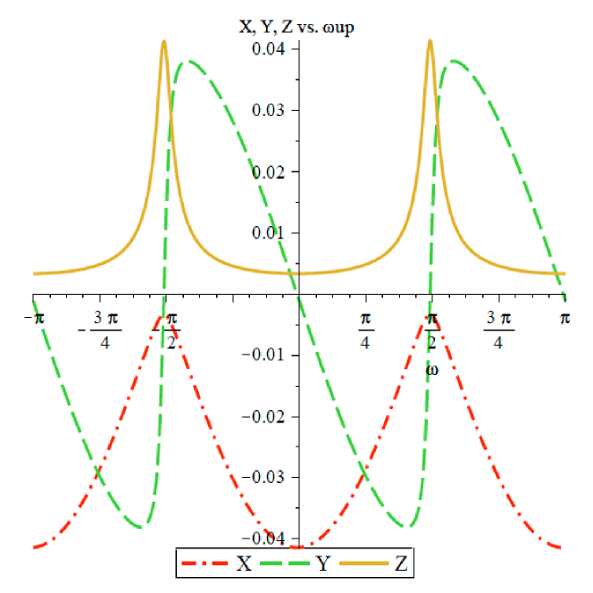
Figure 1: Variation of combined BSM parameters for real and imaginary contributions to CKM matrix as functions of $\omega_{u}$.

V.4 Inverting Definitions

It is possible to invert the sequence of definitions of these quantities and return to the original $y_{i}$ in Eq.(LABEL:eq:Mintz). The result is somewhat cumbersome, but reduces the number of independent parameters to be considered. Explicitly, we can set

$$y2 = y5-y7\;\;\;\;{\rm and}$$

$$y5-y7 = 0$$ (148)

These eliminate two of the imaginary terms in Eq.(LABEL:eq:Mintz) so that this intermediate form of the mass matrix becomes :

$${\mathcal{M}}_{intalt}=\left[\begin{array}[]{ccc}0&0&0\\ 0&0&0\\ 0&0&1\\ \end{array}\right]+\epsilon\times$$ (152)

$$\left[\begin{array}[]{ccc}\sqrt{\frac{2}{3}}y_{0}-\sqrt{\frac{1}{3}}y_{8}+\frac{1}{3}(y_{1}-2y_{4p6})&\frac{1}{\sqrt{3}}(-y_{3}+y_{4m6})&\sqrt{\frac{2}{3}}y_{8}+\frac{1}{3\sqrt{2}}(2y_{1}-y_{4p6}-\sqrt{2}Iy_{9})\\ \frac{1}{\sqrt{3}}(-y_{3}+y_{4m6})&\sqrt{\frac{2}{3}}y_{0}+\frac{1}{\sqrt{3}}y_{8}-y_{1}&-\frac{1}{\sqrt{6}}(2y_{3}+y_{4m6})\\ \sqrt{\frac{2}{3}}y_{8}+\frac{1}{3\sqrt{2}}(2y_{1}-y_{4p6}+\sqrt{2}Iy_{9})&-\frac{1}{\sqrt{6}}(2y_{3}+y_{4m6})&1+\delta-2\sqrt{\frac{2}{3}}y_{0}+\frac{2}{3}(y_{1}+y_{4p6})\\ \end{array}\right]$$ (156)

where we have replaced the labels for the equal quantities $y_{5}$ and $y_{7}$ by $y_{9}$. (Recall that $\xi$ does not appear as we fixed its value by the condition that the trace of ${\mathcal{M}}_{intalt}$ must be equal to the trace of the (scale removed) diagonal matrix of eigenvalues.)

Note that this procedure is not identical to the phase adjustments we made use of above. There the surviving real quantities in the mass matrix included contributions from the imaginary quantities through a normalization factor. In this truncated form, we can identify

$$y_{a} = \frac{1}{\sqrt{3}}(y_{3}-y_{4m6})$$

$$y_{b} = \frac{1}{3\sqrt{2}}\sqrt{(2\sqrt{3}y_{8}+2y_{1}-y_{4p6})^{2}+36y_{9}^{2}}$$

$$y_{c} = \frac{1}{\sqrt{6}}(2y_{3}+y_{4m6})$$ (157)

and recall the unaltered $y_{f}=\frac{1}{\sqrt{3}}y_{8}-\frac{1}{3}(2y_{1}-y_{4p6}).$

Using Eqs.(58, 90, 93, 94) and the assumptions in Eq.(148), we can simplify and invert those relations to obtain

$$2y_{1}-y_{4p6} = \sqrt{3}y_{8}-\frac{3}{2}(1-\delta){\rm cos}(2\omega)$$ (158)

$$y_{4m6} = y_{3}-\frac{\sqrt{3}}{2}(1-\delta){\rm sin}(2\omega)$$ (159)

That is, we can rewrite these combinations of non-Cartan parameters in terms of $y_{3}$ and $y_{8}$ along with a dependence on $\omega$. (As $\omega_{d}=\omega_{u}+\Theta_{C}$, this is still dependence on only a single angle, $\omega=\omega_{u}$.) Since only the combinations on the $lhs$ appear, the separate values of $y_{1}$, $y_{4}$ and $y_{6}$ need not be specified. This provides an example of how the parameters must be related in any BSM model.

VI Discussion

The most striking result of the view espoused here is that the smallness of the non-Cabibbo mixing follows from the ratio of the middle to largest masses of the quarks. Both are due to the perturbative size of BSM corrections to the initial “democratic” starting point. In contrast, the relatively large size of the Cabibbo mixing is allowed by the diagonalization process. A surprising result is that the BSM perturbations need not include all Cartan sub-algebra components, contrary to common analyses, while conversely, non-Cartan sub-algebra BSM perturbations are necessary.

The mass ratios of the quarks are scale dependent, and one could examine the effects of that scale dependence on the CKM matrix and our fit. However, even the ratios are generally not that well known and do not vary significantly with scale over the range from 2 GeV, where the lightest quark masses are generally defined and determined, to the scale of the $b$-quark, nor from there to the weak scale which is also very close to the top quark mass. Refinements responding to these issues are certainly warranted, but we do not expect them to produce large corrections to our BSM parameter constraints determined here. In fact, since the effects considered here are dominated by the values of $\epsilon$, only the uncertainties associated with the masses of the strange and charmed quarks should be significant, as the $b$- and $t$-quark masses are relatively accurately known. Fortunately, the very large uncertainties associated with the ratios of the two lightest quarks do not play a significant role in establishing the configuration, although they will be important for precision analyses.

We have carried out the straightforward extension of our results to the next higher order in $\epsilon$ which might, in principle, be able to further constrain the values of the unknown parameters. Unfortunately, utilization requires knowledge of the relevant experimental values to order $\epsilon^{2}$, i.e., to of order parts in $10^{4}$, which is an accuracy generally not presently available. More accurate measurements would certainly change this conclusion.

VI.1 BSM contributions

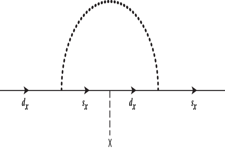
Figure 2: A BSM loop correction to the fermion-Higgs-boson vertex that alters the charged fermion mass matrix from “democratic” to that shown in Eq.(39). Left-chiral fermions with weak interactions are labelled $d_{x}$ for “doublet” and right-chiral fermions with no weak interactions are labelled $s_{x}$ for “singlet” or “sterile”.

In general terms, Fig.(2) shows the nature of expected BSM corrections that could distinguish the different fermions and lead to the small corrections that we find in our fits. The Lagrangian structure that we have in mind uses Weyl spinors for the separate left-chiral ($d_{x}$, for member of a weak interaction doublet) and right-chiral ($s_{x}$, for a weak interaction singlet) parts of the fermion Dirac bispinors, but nonetheless produces Dirac mass terms which may be simply represented as above.

Interestingly, we expect these loop calculations to be finite as they involve only differences within the triples of fermions. This effect was observed in Ref.GG , where a symmetric, overall divergence appears but the differences in mass corrections are finite, although that model is for a quite different application of symmetry-breaking mass corrections and employed vector gauge bosons. Although the calculation there was done only for Cartan sub-algebra corrections, it is not unreasonable to expect that the off-diagonal corrections will also be finite. Note that without the intermediation of the Higgs scalar vacuum expectation value, the $d_{x}$ is not changed to an $s_{x}$ which prevents completion of the loop.

Fig.(2) is drawn for a BSM scalar boson interaction, but a BSM vector could in principle also couple both the Weyl spinor $d_{x}$ to a Weyl spinor $d_{x}$ and similarly $s_{x}$ to $s_{x}$. This simply requires interchanging the labels on either side of the Higgs’ coupling to complete the loop. Again, without the intermediation of the Higgs scalar vacuum expectation value, both the $d_{x}$ and the $s_{x}$ pass through the loop unchanged without coupling to mass, so the BSM correction affects only vertex renormalization.

VI.2 Leptons

Of course, application to the leptons also comes to mind. For the charged leptons, Fig.(2) still applies, as it also does for Dirac mass terms for neutrinos. However, producing these for the neutrinos requires the existence of uncharged Weyl (right-chiral) fermions with no SM interactions at all, i.e., the so-called “sterile” neutrinos, as opposed to the known ones which are “active” with respect to the weak interactions. Under the long honored assumption of quark-lepton (Zweig-Glashow) symmetry, the existence of these states has been widely presumed since the early days of Grand Unified Theories SO10 , starting with $SO(10)$. Aside from the prediction of the charm quark, this symmetry (or regularity) successfully predicted the existence of the $t$- and $b$-quarks as soon as the $\tau$-lepton was discovered. Perl There may even be some recent experimental evidence for “sterile” neutrinos. MiniBooNE

Furthermore, with the discovery COBE of “Dark matter” in the Universe, it is clear that there are additional particles beyond those in the SM and that these particles are sterile. However many different types there are, only three distinct Weyl spinor combinations of these degrees of freedom are required to couple to the active neutrino Weyl spinors in conjunction with the Higgs boson to produce Dirac mass terms for the neutrinos. There is also no impediment for these sterile fields to acquire Majorana masses independently of the Higgs.

It follows that a $6\times 6$ structure in terms of Weyl spinors is required, rather than the simple $3\times 3$ Dirac mass structure that the charged fermions can be reduced to by the standard construction of Dirac bispinors. (Any additional sterile fermions can be block-diagonalized away, leaving the three needed, albeit perhaps of a complex structure in terms of the original model degrees of freedom.) The Dirac mass terms of the neutrinos, $m_{D}$, have the same form as that for the charged fermions as described above, but they now appear in $3\times 3$ off-diagonal blocks in this $6\times 6$ matrix. The upper left $3\times 3$ block remains zero, as the SM does not produce Majorana masses for the active neutrinos, nor is it necessary for BSM physics to do so directly: The “see-saw” mechanism seesaw produced by a sufficiently massive lower right $3\times 3$ block of “sterile” neutrinos leads to light, Majorana mass eigenstates that are dominated by active neutrino amplitudes.

That lower right $3\times 3$ block of Majorana masses (with a structure as given in Eq.(11) above) for the “sterile” Weyl spinors (corresponding to what would have been the right-chiral component of a normal Dirac neutrino wavefunction) is unconstrained. As we pointed out many years ago CoralGables , neutrino mass mixing of the almost purely “active” eigenstates can be expected to be similar to that for the quarks, unless there is some particular structure to this $3\times 3$ block of Majorana masses for the “sterile” Weyl spinors; i.e., barring any special circumstances, the leptonic analog of the $CKM$ matrix, namely the $PMNS$-matrix PMNS , should be similar to the $CKM$ matrix.

At that time, the concern was to determine whether or not neutrinos should be expected to have mass and whether or not their mixing should be expected to be large enough to measure. As we now know, the masses are very small but the mixing is even larger than for the quarks and very close to the particular TBM form that we showed above applies separately to the up- and down-type quarks, but cancels in the $CKM$ matrix.

We have identified a $6\times 6$ to $3\times 3$ block-diagonalization procedure that provides for a determination of the relations required between the sterile neutrino Majorana mass matrix and the BSM parameters in the neutrino Dirac mass matrix, so that, in the diagonalized $6\times 6$ mass matrix, there is negligible mixing of the active parts of the mostly active Majorana mass eigenstates relative to their initial structure. That is, for the leptonic weak interaction currents, we have ascertained that the conditions required, so that the factor contributed by neutrinos to the $PMNS$-matrix is the identity (or close to it), may be satisfied. It follows that, under those conditions, the $PMNS$-matrix for the weak lepton currents will be almost, but not exactly, of the $TBM$ form with small corrections certainly coming from the diagonalization of the charged leptons, which may even be the dominant corrections:

$$PMNS\approx TBM.$$ (160)

This is consistent with current experiments which show that the $PMNS$-matrix is indeed quite close to the $TBM$-matrix form, but the quantity $\theta_{13}$, that vanishes in the exact limit, is not zero dayabay .

If the constraints determined in our $6\times 6$ to $3\times 3$ block-diagonalization procedure are satisfied, then the “democratic” plus BSM hypothesis for the fermion mass matrices would provide a unified understanding of all of the weak current mixing structures simultaneously, subject to those additional constraints on BSM physics being satisfied. Conversely, any model of BSM physics that satisfies these relations will produce the result in Eq.(160). We will present a detailed analysis of the leptonic sector in a future paper.

VII Conclusion

We have started from the assumption that within the SM, for the fermions with a given electric charge, the Higgs doublet is sensitive only to the quantum numbers of the left-chiral Weyl spinor parts of the Dirac wave functions. With this assumption, a basis can be chosen so that the iso-singlet terms formed between them and the Higgs doublet couple equally to all of the right-chiral Weyl spinor parts. This in turn implies that the SM mass matrix should have a “democratic” form, with one massive eigenstate and two massless ones. Upon adding perturbative corrections of a completely general form, presumed to arise from BSM physics, we find that a consistent set of parameters may be extracted that conforms to the known quark mass spectra and CKM mixing matrix, including $CP$-violation. These parameter value constraints provide information on matrix elements of the manner in which BSM physics couples to SM degrees of freedom. The question of why the overall mass scale for the up-quarks is significantly larger than that for the down-quarks remains unresolved, but can be accommodated if there are a pair of Higgs bosons, as is required in supersymmetric models, for example.

It is clear that, in this approach, extracting more detailed information on the nature of BSM physics and the value of BSM matrix elements requires a more accurate determination of the quark mass ratios and their mixing amplitudes in the weak interaction. It would be of great value if the separate real and imaginary parts of the CKM matrix elements could be determined experimentally.

Under the “see-saw” assumption regarding the existence and nature of sterile neutrino components, the extension of these ideas to leptons can also produce the beginning of an understanding as to both why the PMNS matrix is approximately of tri-bi-maximal form and also why it is not exactly so. Along with the information from the violations of “democracy”, the potential information on the sterile neutrino mass matrix may open the door to learning about the physics in the dark matter sector, with the sterile neutrinos as the first component known from other than gravitational interactions.

Finally, we note that the intermediate propagation of sterile as well as active neutrinos in variations of the graphs above applied to weak decay box graphs may be relevant to recent observations of violations of lepton universality, such as in Ref.(TestLeptUniv ).

VIII Acknowledgments

This work was carried out in part under the auspices of the National Nuclear Security Administration of the U.S. Department of Energy at Los Alamos National Laboratory under Contract No. DE-AC52-06NA25396. We thank Bill Louis, Geoff Mills, Richard Van de Water, Dharam Ahluwalia, Alan Kostelećky, Earle Lomon, Rouzbeh Allahverdi, Kevin Cahill, Ami Leviatan and Xerxes Tata for useful conversations.

References

- (1) H. Harari, Phys. Lett. B86 (1979) 83; M. A. Shupe, Phys. Lett. B 86 (1979) 87; Haim Harari and Nathan Seiberg, Nucl. Phys. B204 (1982) 141. See also, P. Zenczykowski, Phys. Lett. B660 (2008) 567.
- (2) Steven Weinberg, Phys. Rev. D 13 (1976) 974; Steven Weinberg, Phys. Rev. D 19 (1979) 1277; Leonard Susskind, Phys. Rev. D 20 (1979) 2619; Savas Dimopoulos and Leonard Susskind, Nucl. Phys. B155 (1979) 237; Bob Holdom, Phys. Rev. D 24 (1981) 1441. See also, Francesco Sannino Act. Phys. Pol. B40 (2009) 3533; arXiv:0911.0931.
- (3) A. Chodos, R. L. Jaffe, K. Johnson and C. B. Thorn, Phys. Rev. D 10 (1974) 2599; T. De Grand, R. L. Jaffe, K. Johnson and J. Kiskis, Phys. Rev. D 12 (1975) 2060.
- (4) V. Alan Kostelecky, private communication.
- (5) H. Georgi and S. L. Glashow, Phys. Rev. Lett. 32 (1974) 438; J. C. Pati and A. Salam, Phys. Rev. D 10 (1974) 275; H. Fritzsch and P. Minkowski, Ann. Phys. 93 (1975) 193; H. Georgi and D. Nanopoulos, Nucl. Phys. B159 (1979) 16; R. N. Mohapatra and B. Sakita, Phys. Rev. D 21 (1980) 1062; F. Wilczek and A. Zee, ibid.25 (1982) 553.
- (6) M. Gell-Mann, P. Ramond, and R. Slansky, in Supergravity, ed. by D. Freedman et al. (North-Holland, Amsterdam, 1980).
- (7) H. Fritzsch, Phys. Lett. 70B (1977) 436.
- (8) There is no recent review and too many papers to reference, so we list only a few recent publications as examples: W. G. Hollik, U. J. Saldana Salazar, Nucl. Phys. B 892 (2015) 364; Zhi-zhong Xing, Int. J. Mod. Phys. A 29 (2014) 1430067; P. V. Dong, N. T. K. Ngan, D. V. Soa, Phys. Rev. D 90 (2014) 075019; F. Hartmann, W. Kilian, Eur. Phys. J. C 74 (2014) 3055; A. E. C rcamo Hern ndez, I. de Medeiros Varzielas, [arXiv:1410.2481]; Priyanka Fakay, [arXiv:1410.7142]; J. Berryman, D. Hern ndez, [arXiv:1502.04140]; I. T. Dyatlov, [arXiv:1502.01501]; E. Nardi, [arXiv:1503.01476].
- (9) Haim Harari, Hervé Haut and Jaques Weyers, Phys. Lett. 78B (1978) 459; Y. Koide, Phys. Lett. 120B (1983) 161; Y. Koide, Phys. Rev. D 28 (1983) 252, Phys. Rev. D39 (1989) 1391; Peter Kaus and Sydney Meshkov, Mod. Phys. Lett. A 3 (1988) 1251, Phys. Rev. D42 (1990) 1863; Morimitsu Tanimoto, Phys. Rev. D41 (1990) 1586; L. Lavoura, Phys. Lett. B228 (1989) 245.
- (10) C. Jarlskog, in Proc. Int. Symp. on Production and Decay of Heavy Flavors, Heidelberg, Germany, 1986, ed. by K. Schubert and R. Waldi, (DESY, Hamburg, 1987), p. 331.
- (11) Zhi-zhong Xing, Deshan Yang and Shun Zhou, Phys. Lett. B690 (2010) 304, but see also, H. Fritzsch and D. Holtmannspötter, Phys. Lett. B338 (1994) 290.
- (12) T. Goldman, G. J. Stephenson Jr. and Bruce H. J. McKellar, J. Phys. : Conf. Ser. 136 (2008) 042023.
- (13) N. Cabibbo, Phys. Rev. Lett. 10 (1963) 531; R. E. Marshak and E. C. G. Sudarshan Phys. Rev. 109 (1958) 1860; M. Gell-Mann and M. évy, Nuovo Cimento 16 (1958) 705.
- (14) M. Kobayashi and T. Maskawa, Prog. Theor. Phys. 49 (1973) 652; L. L. Chau, Phys. Repts. 95 (1983) 1.
- (15) J. Beringer et al., Phys. Rev. D 86 (2012) 010001.
- (16) Z. Maki, M. Nakagawa and S. Sakata, Prog. Theor. Phys. 28 (1962) 870; B. Pontecorvo, Zh. Eksp. Theo. Fiz. 34 (1957) 247 [Sov. Phys. JETP 7 (1958) 172]; Zh. Eksp. Theo. Fiz. 53 (1967) 1717; [Sov. Phys. JETP 26 (1968) 984].
- (17) Z. Z. Xing, H. Zhang and Shun Zhou, Phys. Rev. D 77 (2008) 113016.
- (18) Ami Leviatan, private communication.
- (19) C. Jarlskog, Phys. Rev. Lett. 55 (1985) 1039.
- (20) Howard Georgi and T. Goldman, Phys. Rev. Lett. 30 (1973) 514.
- (21) R. Slansky, Phys. Repts. 79 (1981) 1; see also, H. Georgi and C. Jarlskog, Phys. Lett. 86B (1979) 297; H. Georgi and D. V. Nanopoulos, Nucl. Phys. B 159 (1979) 16; J. A. Harvey, P. Ramond and D. B. Reiss, Phys. Lett. 92B (1980) 309; J. A. Harvey, D. B. Reiss and P. Ramond, Nucl. Phys. B 199 (1982) 223.
- (22) M. L. Perl et al., Phy. Rev. Lett. 35 (1975) 1489.
- (23) A. Aguilar et al., Phys. Rev. D 64 (2001) 112007; A. A. Aguilar-Arevalo et al., Phys. Rev. Lett. 110 (2013) 161801.
- (24) G. Smoot et al. , Ap. J. Lett. 396 (1992) L1; E. L. Wright et al. , ibid L13.
- (25) T. Goldman and G. J. Stephenson, Jr. , Phys. Rev. D 24 (1981) 236.
- (26) F. P. An et al. (Daya Bay Collaboration), Phys. Rev. Lett. 113 (2014) 141802.
- (27) R. Aaij et al. (LHCb Collaboration), Phys. Rev. Lett. 113 (2014) 151601.