Constraining the radio-loud fraction of quasars at $z>5.5$

Abstract

Radio-loud Active Galactic Nuclei at $z\sim 2-4$ are typically located in dense environments and their host galaxies are among the most massive systems at those redshifts, providing key insights for galaxy evolution. Finding radio-loud quasars at the highest accessible redshifts ($z\sim 6$) is important to study their properties and environments at even earlier cosmic time. They would also serve as background sources for radio surveys intended to study the intergalactic medium beyond the epoch of reionization in H I 21 cm absorption. Currently, only five radio-loud ($R=f_{\nu,5{\rm GHz}}/f_{\nu,4400\textup{\AA}}>10$) quasars are known at $z\sim 6$. In this paper we search for $5.5\lesssim z\lesssim 7.2$ quasars by cross–matching the optical Pan-STARRS1 and radio FIRST surveys. The radio information allows identification of quasars missed by typical color-based selections. While we find no good $6.4\lesssim z\lesssim 7.2$ quasar candidates at the sensitivities of these surveys, we discover two new radio-loud quasars at $z\sim 6$. Furthermore, we identify two additional $z\sim 6$ radio-loud quasars which were not previously known to be radio-loud, nearly doubling the current $z\sim 6$ sample. We show the importance of having infrared photometry for $z>5.5$ quasars to robustly classify them as radio-quiet or radio-loud. Based on this, we reclassify the quasar J0203+0012 ($z=5.72$), previously considered radio-loud, to be radio-quiet. Using the available data in the literature, we constrain the radio-loud fraction of quasars at $z\sim 6$, using the Kaplan–Meier estimator, to be $8.1^{+5.0}_{-3.2}\%$. This result is consistent with there being no evolution of the radio-loud fraction with redshift, in contrast to what has been suggested by some studies at lower redshifts.

I. INTRODUCTION

The study of $z\sim 6$ quasars has shown the presence of almost complete Gunn–Peterson absorption troughs in their spectra, corresponding to Ly$\alpha$ absorption by the neutral Hydrogen in the intergalactic medium (IGM). This indicates a rapid increase in the neutral fraction of the IGM above $z>6$, providing strong constraints on the end of the epoch of reionization (EoR) (Fan et al., 2006a). The study of the IGM through Gunn–Peterson absorption has its limitations: quasar spectra suffer from saturated absorption at $z\gtrsim 6$, and thus it becomes increasingly difficult to study the IGM during the EoR (e.g., Furlanetto et al., 2006).

On the other hand, the 21 cm line (unlike the Ly$\alpha$ line) does not saturate, allowing the study of the IGM even at large neutral fractions of Hydrogen (e.g., Carilli et al., 2004a). Therefore, the identification of radio-loud sources at the highest redshifts will be critical for current and future radio surveys. These objects will serve as background sources to study the intergalactic medium beyond the EoR through 21 cm absorption measurements (for example the Low-Frequency Array and the Square Kilometer Array; e.g., see Carilli et al., 2002).

Typical high-redshift quasar searches are based on strict optical and near-infrared color criteria chosen to avoid the more numerous cool dwarfs which have similar colors to high-redshift quasars (e.g., Fan et al., 2001). An alternative to find elusive quasars with optical colors indistinguishable from stars is to require a radio detection. Most of the cool stars that could be confused with high-redshift quasars are not radio–bright at mJy sensitivities (Kimball et al., 2009); therefore, complementing an optical color-based selection with a bright radio detection reduces the contamination significantly (e.g., McGreer et al., 2009).

Currently, there are only three $z>5.5$ quasars known with 1.4 GHz peak flux density $>1$ mJy (J0836+0054, $z=5.81$, Fan et al. 2001; J1427+3312, $z=6.12$, McGreer et al. 2006, Stern et al. 2007; and J1429+5447, $z=6.18$, Willott et al. 2010a). There are two other $z\sim 6$ quasars in the literature classified as radio-loud, but with fainter radio emission (J2228+0110, $z=5.95$, Zeimann et al. 2011; and J0203+0012, $z=5.72$, Wang et al. 2008).

This small sample of currently identified radio-loud quasars at $z\sim 6$ has already provided important insights into Active Galactic Nuclei (AGN) and galaxy evolution, emphasizing the importance of finding more of such objects. For example, there is evidence that a radio–loud $z\sim 6$ quasar might be located in an overdensity of galaxies (Zheng et al., 2006), similar to what has been found in radio-loud AGN at lower redshifts (e.g., Wylezalek et al., 2013). It has also been shown that another $z\sim 6$ radio–loud quasar resides in one of the most powerful known starbursts at $z\sim 6$ (Omont et al., 2013).

At lower redshifts, it is well established that roughly 10% – 20% of all quasars are radio-loud. It has been suggested that the radio-loud fraction (RLF) of quasars is a function of both optical luminosity and redshift (e.g., Padovani, 1993; La Franca et al., 1994; Hooper et al., 1995). If a differential evolution between radio-quiet and radio-loud quasars exists, it could indicate changes in properties of black holes such as accretion modes, black hole masses, or spin (Rees et al., 1982; Wilson & Colbert, 1995; Laor, 2000). This could provide insights into why some quasars have strong radio emission, while most have only weak radio emission.

Some studies have found evidence of such evolution. In particular, Jiang et al. (2007) find that the RLF decreases strongly with increasing redshift at a given luminosity. For example, they find that the RLF at $M_{2500}=-26$ declines from 24% to 4% as redshift increases from 0.5 to 3. Kratzer & Richards (2014) find a behavior in agreement with these findings in a similar redshift range ($z\sim 0.5-2.5$), but they also point out that the evolution of the RLF closely tracks the apparent magnitudes, which suggests a possible bias in the results. However, these results are in stark contrast to other studies finding little or no evidence of such evolution (e.g., Goldschmidt et al., 1999; Stern et al., 2000; Ivezić et al., 2002; Cirasuolo et al., 2003).

In this paper we take advantage of the large area coverage and photometric information provided by the Faint Images of the Radio Sky at Twenty cm survey (FIRST; Becker et al., 1995) and the Panoramic Survey Telescope & Rapid Response System 1 (Pan-STARRS1, PS1; Kaiser et al., 2002, 2010) to search for radio-loud quasars at $5.5\lesssim z\lesssim 7.2$. We also revisit the issue of a possible evolution of the RLF of quasars with redshift by studying the RLF of quasars at the highest accessible redshifts, where an evolution (if existent) should be most evident.

The paper is organized as follows. We briefly describe the catalogs used for this work in Section II. The color selection procedures for $5.5\lesssim z\lesssim 6.4$ and $z\gtrsim 6.4$ quasars with radio counterparts are presented in Section III. In Section 4, we present our follow-up campaign and the discovery of two new radio-loud $z\gtrsim 5.5$ quasars. The radio-loud definition used in this paper and details on how it is calculated are introduced in Section V. In Section VI, we investigate the radio-loud fraction of $z>5.5$ quasars by compiling radio information on all such quasars currently in the literature. This work identifies two additional high-redshift, radio-loud quasars that had not previously been noted to be radio-loud.

We summarize our results in Section VII. Magnitudes throughout the paper are given in the AB system. We employ a cosmology with $H_{0}=69.3\,\mbox{km s}^{-1}$ Mpc^-1, $\Omega_{M}=0.29$, and $\Omega_{\Lambda}=0.71$ (Hinshaw et al., 2013).

II. Survey Data

II.1. FIRST

The FIRST survey was designed to observe the sky at 20 cm (1.4 GHz) matching a region of the sky mapped by the Sloan Digital Sky Survey (SDSS; York et al., 2000), covering a total of about $10,600$ square degrees. The survey contains more than $900,000$ unique sources, with positional accuracy to $\lesssim 1\arcsec$. The catalog has a 5$\sigma$ detection threshold which typically corresponds to 1 mJy although there is a deeper equatorial region where the detection threshold is about 0.75 mJy.

II.2. Pan-STARRS1

The PS1 $3\pi$ survey has mapped all the sky above declination $-30^{\circ}$ over a period of $\sim 3$ years in five optical filters $g_{\rm P1}$, $r_{\rm P1}$, $i_{\rm P1}$, $z_{\rm P1}$, and $y_{\rm P1}$ (Stubbs et al., 2010; Tonry et al., 2012). The PS1 catalog used in this work comes from the first internal release of the $3\pi$ stacked catalog (PV1), which is based on the co-added PS1 exposures (see Metcalfe et al., 2013). This catalog includes data obtained primarily during the period 2010 May–2013 March and the stacked images consist on average of the co-addition of $\sim 8$ single images per filter. The $5\sigma$ median limiting magnitudes of this catalog are $g_{\rm P1}=22.9$, $r_{\rm P1}=22.8$, $i_{\rm P1}=22.6$, $z_{\rm P1}=21.9$, and $y_{\rm P1}=20.9$. PS1 goes significantly deeper than SDSS in the $i$ and $z$ bands which together with the inclusion of a near-infrared $y$ band allow it to identify new high-redshift quasars even in areas already covered by SDSS.

III. Candidate Selection

III.1. The FIRST/Pan-STARRS1 catalog

In this paper we use the multiwavelength information and large area coverage of the FIRST and Pan-STARRS1 surveys to find radio-loud high-redshift quasars. We cross match the FIRST catalog (13Jun05 version) and the PV1 PS1 stack catalog using a 2″ matching radius. This yields a catalog containing $334,290$ objects. Given the similar astrometric accuracy of Pan-STARRS1 and SDSS, we use the same matching radius utilized by the SDSS spectroscopic target quasar selection (Richards et al., 2002). The peak of the SDSS-FIRST positional offsets occurs at $\sim 0.2\arcsec$ and the fraction of false matches within 2″ is about 0.1% (Schneider et al., 2007, 2010, see their Figure 6). Although this matching radius introduces a bias against quasars with extended radio morphologies (e.g., double-lobe quasars without radio cores or lobe-dominated quasars), Ivezić et al. (2002) show that less than 10% of SDSS-FIRST quasars have complex radio morphologies.

As redshift increases, the amount of neutral hydrogen in the universe also increases. At $z\gtrsim 6$ the optically thick Ly$\alpha$ forest absorbs most of the light coming from wavelengths $\lambda_{{\rm rest}}<1216$ Å. This implies that objects at $z\sim 7$ ($z\sim 6$) are undetected or very faint in the $z$-band ($i$-band), showing a ‘drop’ in their spectra. They are thus called $z$-dropouts ($i$-dropouts). This ‘drop’ can be measured by their red $z-y$ and $i-z$ colors for $z$-dropouts and $i$-dropouts, respectively.

Given that the radio detection requirement significantly decreases the amount of contaminants (especially cool dwarfs), we perform a much broader selection criteria in terms of colors and signal-to-noise ratio (S/N) in comparison with our $z$- and $i$-dropout criteria presented in Venemans et al. (2015) and Bañados et al. (2014), respectively. In particular for the $z$-dropouts in this paper, we allow for objects undetected in the $z_{\rm P1}$ band to be 0.1 mag bluer than in Venemans et al. (2015) and relax the S/N criteria in their $g_{\rm P1}$ and $r_{\rm P1}$ bands to be $\mathrm{S/N}<5$ instead of $\mathrm{S/N}<3$ (see Section III.2). For the $i$-dropouts in this paper, we relax the selection limits in comparison with Bañados et al. (2014). We allow the candidates to be 0.7 mag and 0.4 mag bluer in the $i_{\rm P1}-z_{\rm P1}$ and $r_{\rm P1}-z_{\rm P1}$ colors, respectively. For this selection we do not put any constrain in $z_{\rm P1}-y_{\rm P1}$ color (see Section III.3). In this way we can detect $z>5.5$ quasars which have similar colors to cool stars that are missed by typical color-based criteria.

III.2. $z$-dropout catalog search ($z\gtrsim 6.4$)

We require that more than 85% of the expected point-spread function (PSF)-weighted flux in the $z_{\rm P1}$ and the $y_{\rm P1}$ bands is located in valid pixels (i.e., that the PS1 catalog entry has PSF_QF $>0.85$). We require a S/N $>7$ in the $y_{\rm P1}$ band and exclude those measurements in the $y_{\rm P1}$ band flagged as suspicious by the Image Processing Pipeline (IPP; Magnier, 2006, 2007) (see Table 6 in Bañados et al. 2014). The catalog selection can be summarized as:

$$\mbox{S/N}(y_{\rm P1})>7$$ (1a)

$$((\mbox{S/N}(z_{\rm P1})\geq 3)\;\mbox{AND}\,(z_{\rm P1}-y_{\rm P1}>1.4))\;\mbox{OR}$$

$$((\mbox{S/N}(z_{\rm P1})<3)\;\mbox{AND}\,(z_{\rm P1,lim}-y_{\rm P1}>1.3))$$ (1b)

$$(\mbox{S/N}(i_{\rm P1})<5)\;\mbox{OR}\;(i_{\rm P1}-y_{\rm P1}>2.0)$$ (1c)

$$(\mbox{S/N}(r_{\rm P1})<5)$$ (1d)

$$(\mbox{S/N}(g_{\rm P1})<5)$$ (1e)

where $z_{\rm P1,lim}$ is the 3$\sigma$ $z_{\rm P1}$ limiting magnitude. This selection yields 66 candidates.

III.3. $i$-dropout catalog search ($5.5\lesssim z\lesssim 6.4$)

Similar to the $z$-dropout catalog search, we require that more than 85% of the expected PSF-weighted flux in the $i_{\rm P1}$ and the $z_{\rm P1}$ bands is located in valid pixels. We require a S/N $>10$ in the $z_{\rm P1}$ band and exclude those measurements flagged as suspicious by the IPP in the $z_{\rm P1}$ band.

We do not put any constraint on the $y_{\rm P1}$ band. This allows us to identify quasar candidates across a broad redshift range ($5.5\lesssim z\lesssim 6.4$) and make better use of the $z_{\rm P1}$ band depth (which is deeper than the $y_{\rm P1}$ band). The $y_{\rm P1}$ information is used later on for the follow-up campaign.

We can summarize the catalog selection criteria as follows:

$$\mbox{S/N}(z_{\rm P1})>10$$ (2a)

$$((\mbox{S/N}(i_{\rm P1})\geq 3)\;\mbox{AND}\,(i_{\rm P1}-z_{\rm P1}>1.5))\;\mbox{OR}$$

$$((\mbox{S/N}(i_{\rm P1})<3)\;\mbox{AND}\,(i_{\rm P1,lim}-z_{\rm P1}>1.0))$$ (2b)

$$(\mbox{S/N}(r_{\rm P1})<3)\;\mbox{OR}\;(r_{\rm P1}-z_{\rm P1}>1.8)$$ (2c)

$$(\mbox{S/N}(g_{\rm P1})<3)\;\mbox{OR}\;(g_{\rm P1}-z_{\rm P1}>1.8)$$ (2d)

where $i_{\rm P1,lim}$ is the 3$\sigma$ $i_{\rm P1}$ limiting magnitude. This query yields 71 candidates.

III.4. Visual Inspection

The number of candidates obtained from Sections III.2 and III.3 are small enough to visually inspect all of them. We use the latest PS1 images available for the visual inspection, which are usually deeper than the images used to generate the PS1 PV1 catalog. We also perform forced photometry on them to corroborate the catalog colors (as described in Bañados et al. 2014), especially when PV1 only reports limiting magnitudes. Thus, we visually inspect all the PS1 stacked, FIRST, and $z_{\rm P1}$ and $y_{\rm P1}$ PS1 single epoch images (where the S/N is expected to be the highest) for every candidate. The most common cases eliminated by visually inspection are PS1 artifacts due to some bad single epoch images, objects that lacked information in the PV1 catalog, and objects with evident extended morphology in the optical images. Based on the visual inspection, we assign priorities for the follow-up. Low-priority candidates are the ones whose PS1 detections look questionable, in the limit of our S/N cut, and/or objects with extended radio morphology which produces slightly positional offsets ($\gtrsim 1\arcsec$) between the optical and radio sources.

III.4.1 $z$-dropouts

Almost all the candidates can be ruled out by their PS1 stack images and/or single epoch images. There are only two objects we cannot completely rule out although there are some lines of evidence pointing us to believe they are unlikely to be quasars. For both PSO J141.7159+59.5142 and PSO J172.3556+18.7734, the $y_{\rm P1}$ detection looks questionable, in the limit of our S/N cut: 7.5 and 7.0, respectively. Their $y_{\rm P1}$ catalog aperture and PSF magnitudes differ by 0.3 and 0.28 mag which could indicate they are extended sources but it is hard to tell at this low S/N. The optical and radio positional offsets are somewhat larger than for most of the candidates: $0.6\arcsec$ and $1.5\arcsec$. All of this combined makes them low priority candidates. The PS1 and FIRST information for these sources is listed in Table 1.

III.4.2 $i$-dropouts

One of the candidates we selected is the known radio-loud quasar J0836+0054 at $z=5.82$ (Fan et al., 2001). Its images look good and we would have followed it up. There are two low-redshift quasars that could have been selected for follow-up, J0927+0203 a quasar with a bright H$\alpha$ line at $\sim 9200$Å  ($z=0.39$; Schneider et al., 2010) and J0943+5417, an Fe ii low-ionization broad absorption line quasar ($z=2.22$; Urrutia et al., 2009). After the visual inspection and literature search, there are 10 remaining candidates, out of which 9 are high priority candidates. Their PS1 and FIRST photometry are listed in Table 1.

IV. Follow-up

IV.1. Imaging

We use a variety of telescopes and instruments to confirm the optical colors and to obtain near-infrared photometry of our candidates, thereby allowing efficient removal of interlopers.

GROND (Greiner et al., 2008) at the 2.2m telescope in La Silla was used to take simultaneous images in the filters $grizJHK$ during 2014 January 24 – February 5. Typical on-source exposure times were 1440 s in the near-infrared and 1380 s in the optical. The ESO Faint Object Spectrograph and Camera 2 (EFOSC2; Buzzoni et al., 1984) and the infrared spectrograph and imaging camera Son of ISAAC (SofI; Moorwood et al., 1998) at the ESO New Technology Telescope (NTT) were used to perform imaging in the $I_{\rm NTT}$ ($i\#705$), $Z_{\rm NTT}$ ($z\#623$), and $J_{\rm NTT}$ bands during 2014 March 2–6 with on-source exposure times of 600 s in the $I_{\rm NTT}$ and $Z_{\rm NTT}$ bands and 300 s in the $J_{\rm NTT}$ band. The data reduction consisted of bias subtraction, flat fielding, sky subtraction, image alignment, and stacking. The photometric zeropoints were determined as in Bañados et al. (2014) and their errors are included in the magnitudes reported in this work. All of our high-priority candidates were photometrically followed up except for one which we directly observed spectroscopically (see next Section). Two low-priority $z$-dropouts and one low-priority $i$-dropout are still awaiting follow-up. Table 2 shows the follow-up photometry of our candidates.

IV.2. Spectroscopy

We have taken spectra of four high-priority objects that were not rejected by the follow-up photometry. We processed the data using standard techniques, including bias subtraction, flat fielding, sky subtraction, combination of individual frames, wavelength calibration, and spectrum extraction. The spectra were flux calibrated using standard stars from Massey & Gronwall (1990) and Hamuy et al. (1992, 1994).

The candidate PSO J114.6345+25.6724 was observed with the FOcal Reducer/low dispersion Spectrograph 2 (FORS2; Appenzeller & Rupprecht, 1992) at the Very Large Telescope (VLT) on 2014 April 26 with an exposure time of 1497 s. The spectrum shows no clear break in the continuum and we classify this object as a radio galaxy at $z=1.17$ by the identification of the narrow [O ii] $\lambda 3728$ emission line.

We obtained an optical spectrum of the candidate PSO J354.6110+04.9453 using the Double Spectrograph on the 5 m Hale telescope at Palomar Observatory (DBSP) on 2014 July 21 for a total integration time of 1800 s. The object has a red spectrum lacking the clear (Ly$\alpha$) break which is a typical signature of high-redshift quasars. The spectrum does not clearly identify lines to determine a redshift. We believe this object is most likely a radio galaxy, but it is definitely not a $z>5.5$ quasar. The other two spectroscopically followed up objects – PSO J055.4244–00.8035 and PSO J135.3860+16.2518 – were confirmed to be high-redshift quasars. These two newly discovered quasars would not have been selected as candidates by the optical selection criteria presented in Bañados et al. (2014) (although PSO J055.4244–00.8035 has only a lower limit of $i_{\rm P1}-z_{\rm P1}>1.3$ and it might have been selected if deeper $i_{\rm P1}$ data was available). The observations for these quasars are outlined in more detail below.

IV.2.1 PSO J055.4244–00.8035 ($z=5.68\pm 0.05$)

The discovery spectrum was taken on 2014 February 22 using the DBSP spectrograph with a total exposure time of 2400 s. These observations were carried out in $\sim 1\arcsec$ seeing using the 1$\farcs$5 wide longslit. This spectrum shows a sharp Ly$\alpha$ break indicating that the object is unambiguously a quasar at $z>5.5$ but the S/N does not allow us to determine an accurate redshift. We took a second spectrum with FORS2 at the VLT on 2014 August 4; the seeing was 1$\farcs$1 and it was observed for 1467 s. This spectrum is shown in Figure 1 and there are no obvious lines to fit and use to derive a redshift. There is, however, a tentative Si iv+ O iv] line which falls in a region with considerable sky emission and telluric absorption making it not reliable for redshift estimation. We estimate the redshift instead by comparing the observed quasar spectrum with the composite SDSS $z\sim 6$ quasar spectrum from Fan et al. (2006b). We assume the redshift that minimizes the $\chi^{2}$ between the observed spectrum and the template (the wavelength range where the minimization is performed is $\lambda_{\rm rest}$ = 1240 – 1450 Å). The estimated redshift is $z=5.68$. However, because of the lack of strong features in the spectrum, the $\chi^{2}$ distribution is relatively flat around the minimum and thus a range of redshifts is acceptable. We follow Bañados et al. (2014) and assume a redshift uncertainty of 0.05.

IV.2.2 PSO J135.3860+16.2518 ($z=5.63\pm 0.05$)

The discovery spectrum was taken with EFOSC2 at the NTT on 2014 March 3. The observations were carried out with the Gr#16 grism, 1$\farcs$5 slit width, 1$\farcs$3 seeing, and a total exposure time of 3600 s. The spectrum is very noisy but it resembles the shape of a high-redshift quasar with a tentative Ly$\alpha$ line at $\sim 8100\,$Å. In order to increase the S/N and confirm the quasar redshift, we took two additional spectra and combined them. One spectrum was taken on 2014 April 5 with the Multi-Object Double Spectrograph (MODS; Pogge et al., 2010) at the Large Binocular Telescope (LBT). The observations were carried out under suboptimal weather conditions with the 1$\farcs$2 wide longslit for a total exposure time of 2400 s. The second spectrum was taken with FORS2 at the VLT on 2014 April 26 with a total exposure time of 1467 s. The observing conditions were excellent with 0$\farcs$55 seeing and we used the 1$\farcs$3 width longslit. The combined MODS-FORS2 spectrum is shown in Figure 1. The estimated redshift by matching to the $z\sim 6$ quasar composite spectrum from Fan et al. (2006b) is $z=5.63\pm 0.05$. The redshift estimate for PSO J135.3860+16.2518 is quite uncertain as represented by its error bar. There might be a tentative Si iv+ O iv] line which would place this quasar at a slightly higher redshift. However, this line falls in the same region as the tentative line in the quasar PSO J055.4244–00.8035, which is not a reliable region for redshift determination. A higher S/N optical spectrum and/or a near-infrared spectrum would be beneficial to obtain a more accurate redshift.

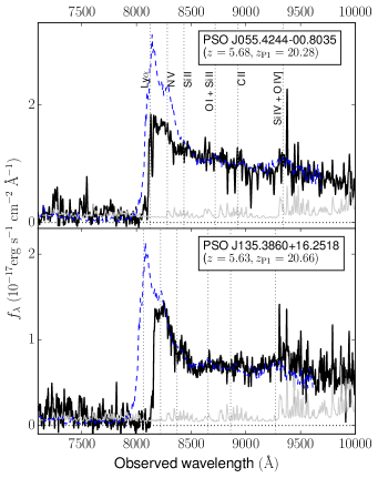
Figure 1.— Spectra of the two radio-loud quasars discovered in this paper. The gray solid lines show the 1$\sigma$ error in the spectra. The blue dashed line is the SDSS $z\sim 6$ composite quasar spectrum from Fan et al. (2006b) at the redshift of the quasars for comparison. Vertical dotted lines indicate the observed wavelengths of key spectral lines, as given in the top panel.

V. Radio-Loudness

A clear consensus on a boundary between radio-loud and radio-quiet quasars has been difficult to achieve and there are several radio-loudness criteria in the literature (for a comparison of the different criteria see Hao et al., 2014). We adopt the most widespread definition in the literature. This is the radio/optical flux density ratio, $R=f_{\nu,5{\rm GHz}}/f_{\nu,4400\textup{\AA}}$ (Kellermann et al., 1989), where $f_{\nu,5{\rm GHz}}$ is the 5 GHz radio rest-frame flux density, $f_{\nu,4400\textup{\AA}}$ is the 4400 Å optical rest-frame flux density, and a quasar is considered radio loud if $R>10$.

V.1. The Radio Emission

The rest-frame $5$ GHz radio flux density is obtained from the observed peak flux density at $1.4$ GHz. We use the peak flux density since most of the $z\sim 6$ quasars appear to be unresolved on the radio maps (e.g., Wang et al., 2007, 2011, but see also Cao et al., 2014, where they claim that there may be extended structures around the radio-loud quasar J2228+0110 on arcsecond scales).

We assume a power-law ($f_{\nu}\sim\nu^{\alpha}$) radio spectral energy distribution, adopting a typical radio spectral index $\alpha_{R}=-0.75$ as used in other high-redshift studies (e.g., Wang et al., 2007; Momjian et al., 2014). This index appears to be appropriate as Frey et al. (2005, 2008, 2011) find that at least three $z\sim 6$ radio-loud quasars show a steep radio spectrum.

V.2. The Optical Emission

The optical spectral indices of quasars span a fairly large range (at least $-1<\alpha_{\nu}<0$). When a direct measurement of the optical rest-frame flux density at 4400 Å is not possible, this is typically extrapolated from the AB magnitude at rest frame 1450 Å ($m_{1450}$) assuming an average optical spectral index of $\alpha_{\nu}=-0.5$ (e.g., Wang et al., 2007). These fairly large extrapolations could lead to dramatic errors if the studied quasars are not average quasars. At $z\sim 6-7$ we can take advantage of infrared space missions such as Spitzer and the Wide-Field Infrared Survey (WISE; Wright et al., 2010) to reduce the extrapolation error by using $\sim 3\,\mu$m ($\lambda_{\rm rest}=4286\textup{\AA}$ at $z=6$) photometry.

Following previous works, we also assume an optical spectral index of $\alpha_{\nu}=-0.5$ but we estimate $f_{\nu,4400\textup{\AA}}$ from IRAC (Fazio et al., 2004) $3.6\mu$m ($S_{3.6\,\mu m}$) observations when available ($\lambda_{\rm rest,eff}=5071$Å at $z=6$). Otherwise, $f_{\nu,4400\textup{\AA}}$ is calculated from the WISE $W_{1}$ magnitude ($\lambda_{\rm rest,eff}=4811$Å at $z=6$) reported in the ALLWISE Source catalog or reject table (with $S/N>2.5$). Table Constraining the radio-loud fraction of quasars at $z>5.5$ lists $S_{3.6\,\mu\rm{m}}$, $W_{1}$, and $m_{1450}$ for all $z>5.5$ quasars with published measurements at $1.4$ GHz in the literature. There are five quasars without IRAC or WISE measurements. For these objects, $f_{\nu,4400\textup{\AA}}$ is estimated from $m_{1450}$. To estimate the error we determine $f_{\nu,4400\textup{\AA}}$ from $m_{1450}$ for the quasars having IRAC or WISE ($\sim 3\,\mu$m) measurements. Then, for each object we compute the ratio $(f_{\nu,4400\textup{\AA}}(3\,\mu\rm{m})-f_{\nu,4400\textup{\AA}}(m_{1450}))/f_{\nu,4400\textup{\AA}}(3\,\mu\rm{m})$. This results in a symmetric distribution, centered on zero, and with a standard deviation of 0.4. Finally, we take the absolute value of the previous distribution and assume its median as a representative error for $f_{\nu,4400\textup{\AA}}$ derived from $m_{1450}$. This corresponds to a relative error of 0.30 (i.e., analogous to assuming a measurement of $f_{\nu,4400\textup{\AA}}$ with $S/N=3.3$). These errors must be taken with caution since they are just representative uncertainties and there could be objects with considerably larger errors, as exemplified in Section VI.1.

VI. Results

We determine the radio-loudness parameter $R$ and the optical and radio luminosities $L_{4400\textup{\AA}}$ and $L_{\rm 5GHz}$ ($L=\nu L_{\nu}$) for all the $z>5.5$ quasars having 1.4 GHz data published in the literature. These parameters are included in Table Constraining the radio-loud fraction of quasars at $z>5.5$. Figure 2 shows the rest-frame 5 GHz radio luminosity versus rest-frame 4400 Å optical luminosity. Eight quasars are classified as radio-loud ($R>10$), including the two quasars discovered in Section IV.2 and two additional possible radio-loud quasars which will be introduced in Section VI.2. There are 33 objects robustly classified as radio-quiet quasars ($R<10$). Two quasars need deeper radio data to classify them unambiguously (with radio loudness upper limit $>10$). In this paper we do not find any radio-loud quasar at $z\sim 7$ in an area of about $10,600$ square degrees of sky to the sensitivities of the FIRST and Pan-STARRS1 surveys ($\sim 1$ mJy and $7\sigma$-limiting magnitude $y_{\rm P1}\sim 20.5$, respectively). Conclusions on the RLF at $z>6.5$ are not possible at this time, since there are currently only seven quasars known at $z>6.5$ (Mortlock et al., 2011; Venemans et al., 2013, 2015). From these seven quasars, only one has dedicated radio follow-up (Momjian et al., 2014) while a second one is in the FIRST footprint but it is a non-detection (see Section VI.3; Venemans et al., 2015). The RLF at $z\sim 6$ is discussed in Section VI.3.

VI.1. J0203+0012: A Radio-Loud Quasar?

The quasar J0203+0012 at $z=5.72$ was classified as radio-loud quasar by Wang et al. (2008). They derived the rest-frame 4400 Å flux density from the 1450 Å  magnitude. As discussed previously, these large extrapolations can carry large uncertainties and can be critical for the classification and derived parameters for specific objects. This is the case for J0203+0012, a broad-absorption line quasar (Mortlock et al., 2009) whose $m_{1450}$ could have been underestimated, resulting in a low optical luminosity (see also its spectral energy distribution in Figure 14 of Leipski et al., 2014). This quasar has a radio-loudness parameter $R=4.3\pm 0.5$ or $R=12.1\pm 3.2$ depending if the rest-frame 4400 Å flux density is extrapolated from the IRAC 3.6 $\mu$m photometry or from $m_{1450}$, respectively (see Figure 2). It is clear that the difference is dramatic and that by using the $m_{1450}$ proxy this quasar would be classified (barely) as radio-loud. We argue that the value of $L_{4400\textup{\AA}}$ obtained from the observed $3.6\,\mu$m photometry is more reliable for $z>5.5$ quasars since it relies less on extrapolation (for this particular case, the extrapolation is less by approximately a factor of three). Also, while radio-loud AGN are typically located in dense environments (e.g., Venemans et al., 2007; Hatch et al., 2014), we found that J0203+0012 does not live in a particularly dense region but rather comparable with what is expected in blank fields (Bañados et al., 2013).

VI.2. Pushing the FIRST Detection Threshold

The FIRST survey has a typical source detection threshold of 1 mJy beam^-1 which assures that the catalog has reliable entries with typical S/N greater than five. There are 30 known $z>5.5$ quasars that are not in the FIRST catalog or in the Stripe 82 VLA Survey catalog (Hodge et al., 2011) but that are located in the FIRST footprint. The discovery papers of these quasars are Mahabal et al. (2005); Cool et al. (2006); Jiang et al. (2009); Willott et al. (2009, 2010a, 2010b); McGreer et al. (2013); Bañados et al. (2014); Venemans et al. (2015); Bañados et al. (in prep.); Venemans et al. (in prep.); and Warren et al. (in prep.).

We checked for a radio detection beyond the FIRST catalog threshold as follows: we obtained the 1.4 GHz FIRST images for all 30 quasars and checked for radio emission within 3″ of the optical quasar position with a S/N$\geq 3$. We find that the quasars J1609+3041 at $z=6.14$ (Warren et al. in prep) and J2053+0047 at $z=5.92$ (Jiang et al., 2009) have tentative 1.4 GHz detections at S/N of 3.5 and 3, respectively. Their radio postage stamps are shown in Figure 3. The two quasars have optical-to-radio positional differences less than 1$\farcs$8 (1 pixel). In order to quantify the probability of finding a spurious association with a $3\sigma$ fluctuation given our sample of 30 quasars we performed the following steps. We placed 100 random positions in each 1 arcmin² FIRST image centered on a quasar and measured the maximum peak flux within 1$\farcs$8. We removed points falling within 1$\farcs$8 from an optical source in the PS1 catalog. There are no radio sources in the FIRST catalog for any of these 1 arcmin² fields. We computed the fraction of measurements with S/N$\,\geq 3$. We repeated this procedure 100 times and the fraction of measurements with S/N$\,\geq 3$ was always $<1\%$. The full distribution is centered on $0.5\%$ with a standard deviation of $0.1\%$. Therefore, in our sample of 30 quasars, the expected number of spurious $\sim 3\sigma$ associations within 1$\farcs$8 is $0.15$ and being conservative less than $0.3$. This analysis suggests that these identifications are unlikely to be spurious. If these detections are real, these quasars are classified as radio-loud with $R=28.3\pm 8.6$ and $R=44.1\pm 18.7$ (see Table Constraining the radio-loud fraction of quasars at $z>5.5$). In Figure 2, these new tentative radio detections are marked as red downward triangles.

We make a mean stack of the 28 remaining quasars in the FIRST footprint that have $\mathrm{S/N}<3$ in their individual images. We find no detection in the stacked image with an upper limit of $f_{\nu}=84\,\mu$Jy (see Figure 2).

VI.3. Constraining the Radio-Loud Fraction of Quasars at $z\sim 6$

Considering all the quasars in Table Constraining the radio-loud fraction of quasars at $z>5.5$, there are eight known radio-loud quasars at $z\sim 6$, 32 radio-quiet (excluding J1120+0641 at $z=7.08$), and two ambiguous. There is one additional quasar that is robustly classified by a non-detection in FIRST as radio–quiet: J0148+0600 at $z=5.98$ (Bañados et al., 2014; Becker et al., 2015). This radio-quiet quasar has $\log L_{4400\textup{\AA}}\,(L_{\sun})=13.04\pm 0.2$, $\log L_{\rm 5\,Ghz}(L_{\sun})<8.7$, and $R<5.6$ (see Figure 2). We can provide a rough estimation of the radio-loud fraction of quasars at $z\sim 6$ of RLF $=8/(8+(34+1))\sim 19\%$. In this statistics we considered the two ambiguous cases as radio-quiet. This is a relatively large fraction; however, these quasars were selected by several methods which could potentially bias the results. As we have included radio-loud quasars that could not have been discovered based on their optical/near-infrared properties alone, the actual fraction of radio-loud quasars is overestimated. Therefore, this value has to be taken only as an upper limit.

In order to set a lower limit in the RLF at $z\sim 6$, we consider quasars that were selected based on their optical properties (i.e., we exclude the two quasars discovered in this paper, J2228+0110 which was discovered by its radio emission by Zeimann et al. 2011, and J1427+3312 which was discovered by its radio emission by McGreer et al. 2006). We also exclude quasars at $z>6.5$, i.e., J1120+0641 at $z=7.08$ and PSO J036.5078+03.0498 at $z=6.527$. The latter quasar was discovered in Venemans et al. (2015). It is not detected in FIRST and has $\log L_{4400\textup{\AA}}\,(L_{\sun})=12.87\pm 0.03$, $\log L_{\rm 5\,Ghz}(L_{\sun})<8.8$, and $R<10.7$ (see Figure 2). Considering all the FIRST non-detections from the previous section as radio-quiet, we find a lower limit of RLF $=4/(4+(34+27))\sim 6\%$. This is a lower limit because there is still the possibility that a fraction of the FIRST non-detections are radio-loud (see Figure 2). Therefore, in this case we are potentially underestimating the number of radio-loud quasars.

Additionally, in order to fully use the information provided by both the radio detections and upper limits, we estimate the radio-loud fraction using the Kaplan–Meier estimator (Kaplan & Meier, 1958). The RLF estimated with this method, after excluding quasars at $z>6.5$ and quasars selected by their radio emission, is $8.1^{+5.0}_{-3.2}\%$.

VI.4. What Changes with an Alternative Radio-Loudness Definition?

Another common definition for radio-loudness in the literature (besides our adopted criteria in Section V), is a simple cut on rest-frame radio luminosity. This criteria is a better indicator of radio-loudness if the optical and radio luminosities are not correlated (Peacock et al., 1986; Miller et al., 1990; Ivezić et al., 2002, Appendix C). We here explore how our results would change if we adopt a fixed radio luminosity as a boundary between radio-quiet and radio-loud objects. We use the alternative criteria adopted by Jiang et al. (2007), where a radio-loud quasar is defined with a luminosity density at rest-frame 5 GHz, $L_{\nu,\rm 5Ghz}>10^{32.5}$ ergs s^-1 Hz^-1. This is equivalent to requiring $\log L_{\rm 5\,Ghz}(L_{\sun})>8.61$ (see the horizonal line in Figure 2).

One caveat with this definition is that J2228+0110 is just below the radio-loud cut although is still consistent with being radio-loud within the uncertainties: $\log L_{\rm 5Ghz}(L_{\sun})=8.59\pm 0.08$. Note that the quasar J0203+0012, discussed in Section VI.1, is also classified as radio-quiet by this definition.

We estimate the radio-loud fraction using the Kaplan–Meier estimator, following the approach of the previous section. The estimated RLF with this definition is $6.6^{+4.1}_{-1.6}\%$. This result agrees with the one obtained in Section  VI.3, and they are both consistent with no strong evolution of the radio-loud fraction of quasars with redshift.

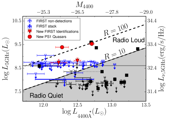
Figure 2.— Rest-frame 5 GHz radio luminosity versus rest-frame $4400$Å optical luminosity for all $z>5.5$ quasars in the literature observed at 1.4 GHz (see Table Constraining the radio-loud fraction of quasars at $z>5.5$). Filled symbols are 1.4 GHz detections and arrows represent $3\sigma$ upper limits in the rest-frame 5GHz luminosity. The dashed lines represent the radio-to-optical ratios ($R$) of 100 and 10 (separation of radio-loud and radio-quiet). The red circles are the two new Pan-STARRS1 radio-loud quasars presented here. These quasars are among the most radio loud quasars at these redshifts. The red downward triangles are two quasars that we identify as radio-loud by inspecting their FIRST images (see Section VI.2). The blue downward triangles are upper limits for 28 quasars that are located in the FIRST survey footprint. The blue upward triangle represents the location of the stack of the 28 undetected quasars in the FIRST survey assuming their average redshift of 6. The gray cross represents the position of J0203+0012 if its $L_{4400\textup{\AA}}$ is calculated from extrapolating $m_{1450}$ and it is connected by a dotted line with the position determined by estimating $L_{4400\textup{\AA}}$ from the IRAC $3.6\,\mu$m photometry (see Section VI.1). The horizontal gray line denotes the division of radio-loud and radio-quiet quasars employed by Jiang et al. (2007) (see Section VI.4).

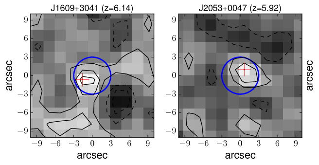
Figure 3.— 1.4 GHz postage stamp images from the FIRST Survey (typical resolution of 5″) of the quasars J1609+3041 (left) and J2053+0047 (right). The blue circles have a radius of 3″ and are centered on the quasar optical positions. These positions have J2000 coordinates corresponding to (R.A., Decl.) = (16:09:37.28, +30:41:47.7) for J1609+3041, and (R.A., Decl.) = (20:53:21.77, +00:47:06.8) for J2053+0047. The red crosses show the 1.4 GHz peak pixel. The black solid (dashed) lines are the positive (negative) $1,2,3\sigma$ -contours. J1609+3041 and J2053+0047 have a S/N of 3.5 and 3.0, respectively. Using these radio flux densities, both quasars are classified as radio-loud with $R=28.3\pm 8.6$ and $R=44.1\pm 18.7$, respectively (see Table Constraining the radio-loud fraction of quasars at $z>5.5$).

VII. Summary

We perform a search for high-redshift, radio-loud quasars ($i$- and $z$-dropouts) by combining radio and optical observations from the FIRST and Pan-STARRS1 surveys. The multiwavelength information of these surveys allows the identification of quasars with optical colors similar to the more numerous cool dwarfs and therefore missed by typical color selection used by high-redshift quasar surveys (e.g., Fan et al., 2006c; Bañados et al., 2014). We do not find good quasar candidates at $z\gtrsim 6.4$ ($z$-dropouts). We discover two of the radio loudest quasars at $z\gtrsim 5.6$: PSO J055.4244–00.8035 ($z=5.68$) with a radio-loudness parameter $R=178.0\pm 40.5$ and PSO J135.3860+16.2518 ($z=5.63$) with $R=91.4\pm 8.8$. These two quasars are at the low-redshift end of the $i$-dropout selection technique ($5.5\lesssim z\lesssim 5.7$) and they are too blue in $i-z$ to have been selected by color cuts usually applied in optical searches for high-redshift quasars. Currently, there is an apparent lack of quasars at $5.2<z<5.7$ (see McGreer et al., 2013; Bañados et al., 2014, their Figure 4). This is due to the similarity between optical colors of quasars and M dwarfs which are the most numerous stars in the Galaxy (Rojas-Ayala et al., 2014). The identification of these two radio-loud quasars in our extended selection criteria implies that there must be a significant number of radio-quiet quasars at these redshifts that are just being missed by standard selection criteria. The use of additional wavelength information, for example using WISE photometry, might help to find quasars in this still unexplored redshift range.

We inspect all the 1.4 GHz FIRST images of the known quasars that are in the FIRST survey footprint but not in the catalog. Based on this inspection, we identify two additional $z\sim 6$ radio-loud quasars which are detected at S/N $\gtrsim 3$ and therefore would benefit from deeper radio imaging.

We highlight the importance of infrared photometry (e.g., from Spitzer or WISE) for $z>5.5$ quasars in order to have an accurate measurement of the rest-frame 4400 Å luminosity which allows us to robustly classify quasars as radio-loud or radio-quiet. By using Spitzer photometry we reclassify the quasar J0203+0012 at $z=5.72$ as radio-quiet ($R=4.3\pm 0.5$). This quasar was previously classified as radio-loud by estimating its rest frame 4400 Å luminosity from the magnitude at 1450 Å (Wang et al., 2008). The estimate based on an infrared proxy is much better than the one based on the $m_{1450}$ proxy because less extrapolation is needed. Thus, the estimated rest-frame 4400 Å luminosity is less affected by spectral energy distribution assumptions.

We compile all the $z>5.5$ quasars having 1.4 GHz data in the literature and, by making simple assumptions (see Section VI.3), we find that the radio-loud fraction of quasars at $z\sim 6$ is between 6% and 19%. We also estimate the radio-loud fraction using the Kaplan–Meier estimator which takes into account both radio detections and upper limits, obtaining RLF$\,=8.1^{+5.0}_{-3.2}\%$. This fraction suggests no strong evolution of the radio-loud fraction with redshift. This result contrasts with some lower redshift studies that show a decrease of the radio-loud fraction of quasars with redshift (e.g., Jiang et al., 2007).

The study of the RLF of quasars at $z\gtrsim 6$ has the potential to give a definitive answer to the issue of a possible evolution of the RLF of quasars with redshift. For this, a homogeneous radio (and infrared) follow-up of a well-defined sample of $z\sim 6$ quasars (or $z\sim 7$ when more of these objects are discovered) selected in a consistent manner is crucial to test whether there is evolution in the RLF of quasars.

Table 1Candidates After Visual Inspection

Candidate	R.A.	Decl.	$g_{\rm P1}$	$r_{\rm P1}$	$i_{\rm P1}$	$z_{\rm P1}$	$y_{\rm P1}$	$S_{\rm 1.4\,GHz,peak}$	Prio.
	(J2000)	(J2000)	(mag)	(mag)	(mag)	(mag)	(mag)	(mJy)
PSO J141.7159+59.5142	09:26:51.83	+59:30:51.2	$>23.69$	$>23.39$	$>23.27$	$>22.71$	$20.64\pm 0.14$	$1.11\pm 0.15$	L
PSO J172.3556+18.7734	11:29:25.36	+18:46:24.3	$>23.64$	$>23.41$	$>23.26$	$>22.78$	$20.68\pm 0.16$	$1.02\pm 0.14$	L
PSO J044.9329–02.9977	02:59:43.91	–02:59:51.9	$>22.81$	$>23.33$	$22.88\pm 0.28$	$21.16\pm 0.08$	$20.89\pm 0.17$	$5.86\pm 0.08$	H
PSO J049.0958–06.8564	03:16:23.00	–06:51:23.2	$>22.57$	$>23.11$	$23.07\pm 0.28$	$21.37\pm 0.10$	$20.76\pm 0.17$	$2.77\pm 0.14$	H
PSO J055.4244–00.8035	03:41:41.86	–00:48:12.7	$>22.88$	$>23.08$	$>21.54$	$20.28\pm 0.05$	$20.27\pm 0.10$	$2.14\pm 0.14$	H
PSO J106.7475+40.4145	07:06:59.40	+40:24:52.3	$>23.57$	$>23.44$	$>22.73$	$21.39\pm 0.10$	$20.85\pm 0.17$	$1.37\pm 0.13$	L
PSO J114.6345+25.6724	07:38:32.30	+25:40:20.8	$>23.55$	$22.95\pm 0.14$	$22.48\pm 0.25$	$20.89\pm 0.10$	$20.62\pm 0.15$	$6.75\pm 0.13$	H
PSO J135.3860+16.2518	09:01:32.65	+16:15:06.8	$23.61\pm 0.24$	$>23.97$	$22.38\pm 0.17$	$20.67\pm 0.05$	$20.82\pm 0.15$	$3.04\pm 0.14$	H
PSO J164.9800+07.4459	10:59:55.22	+07:26:45.5	$>23.08$	$>22.68$	$21.71\pm 0.14$	$20.17\pm 0.05$	$>21.39$	$3.35\pm 0.14$	H
PSO J208.4897+11.8071	13:53:57.54	+11:48:25.6	$>23.46$	$23.27\pm 0.28$	$22.73\pm 0.15$	$20.96\pm 0.09$	$20.79\pm 0.14$	$2.28\pm 0.13$	H
PSO J238.0370–03.5494	15:52:08.89	–03:32:58.0	$>23.57$	$>23.6$	$22.85\pm 0.33$	$21.15\pm 0.07$	$20.84\pm 0.19$	$6.01\pm 0.15$	H
PSO J354.6110+04.9453	23:38:26.65	+04:56:43.3	$>23.46$	$23.01\pm 0.19$	$22.77\pm 0.18$	$20.88\pm 0.09$	$20.98\pm 0.29$	$6.44\pm 0.13$	H

Note. — The two entries at the top are $z$-dropouts and the ten at the bottom are $i$-dropouts. The lower limits correspond to $3\sigma$ limiting magnitudes.

Table 2High Priority $i$-dropout Candidates Follow-up.

Candidate	$g_{\rm GROND}$	$r_{\rm GROND}$	$i_{\rm GROND}$	$z_{\rm GROND}$	$J_{\rm GROND}$	$H_{\rm GROND}$	$K_{\rm GROND}$	$I_{\rm NTT}$	$Z_{\rm NTT}$	$J_{\rm NTT}$	Note
	(mag)	(mag)	(mag)	(mag)	(mag)	(mag)	(mag)	(mag)	(mag)	(mag)
PSO J044.9329–02.9977	$>23.72$	$23.37\pm 0.29$	$22.20\pm 0.18$	$22.14\pm 0.23$	$20.35\pm 0.17$	$19.92\pm 0.17$	$19.20\pm 0.28$	–	–	–	3
PSO J049.0958–06.8564	$24.47\pm 0.33$	$23.90\pm 0.23$	$23.12\pm 0.26$	$21.98\pm 0.12$	$20.52\pm 0.15$	$20.01\pm 0.18$	$19.19\pm 0.24$	–	–	–	3
PSO J055.4244–00.8035	$>23.73$	$>23.77$	$22.16\pm 0.18$	$20.58\pm 0.05$	$20.08\pm 0.16$	$20.03\pm 0.22$	$>19.09$	–	–	–	1
PSO J114.6345+25.6724	–	–	–	–	–	–	–	$22.04\pm 0.18$	$20.95\pm 0.28$	$20.48\pm 0.11$	2
PSO J135.3860+16.2518	$>24.57$	$24.32\pm 0.36$	$22.70\pm 0.18$	$20.85\pm 0.04$	$20.30\pm 0.12$	$20.91\pm 0.33$	$>19.71$	–	–	–	1
PSO J164.9800+07.4459	$23.66\pm 0.15$	$22.19\pm 0.06$	$21.15\pm 0.05$	$20.49\pm 0.02$	$19.96\pm 0.10$	$19.72\pm 0.13$	$19.45\pm 0.27$	$20.64\pm 0.04$	$20.27\pm 0.04$	–	3
PSO J208.4897+11.8071	$>24.50$	$23.21\pm 0.18$	$22.08\pm 0.25$	$21.66\pm 0.11$	$20.53\pm 0.23$	$19.83\pm 0.19$	$>19.46$	–	–	–	3
PSO J238.0370–03.5494	$>24.47$	$23.44\pm 0.18$	$22.03\pm 0.11$	$21.32\pm 0.07$	$19.99\pm 0.11$	$19.74\pm 0.16$	$>19.70$	–	–	–	3
PSO J354.6110+04.9453	–	–	–	–	–	–	–	–	–	–	2

Note. — The magnitude lower limits correspond to $3\sigma$ limiting magnitudes.

Table 3Data and Derived Parameters of the $z>5.5$ Quasars with 1.4GHz Data in the Literature.

Quasar	$z$	$S_{\rm 1.4\,GHz,peak}$	Ref.($z$,1.4 GHz)	$m_{1450}$	$W_{1}$	$S_{3.6\mu\rm{m}}$	$\log L_{5\,{\rm GHz}}$	$\log L_{4400\textup{\AA}}\tablenotemark{d}$	$R$
		($\mu\rm{Jy}$)		(mag)	(mag)	(mag)	($L_{\sun}$)	($L_{\sun}$)
J0002+2550	5.82	$89\pm 14$	1,2	19.0	$18.86\pm 0.06$	$18.71\pm 0.02$	$8.03\pm 0.07$	$13.05\pm 0.01$	$1.3\pm 0.2$
J0005–0006	5.85	$<390$	3,4	20.2	$20.00\pm 0.16$	$20.10\pm 0.03$	$<8.7$	$12.49\pm 0.01$	$<20.9$
J0033–0125	6.13	$<57$	5,4	21.8	$20.99\pm 0.40$	–	$<7.9$	$12.19\pm 0.15$	$<6.8$
J0203+0012	5.72	$195\pm 22$	6,4	21.0	$19.39\pm 0.09$	$19.14\pm 0.03$	$8.36\pm 0.05$	$12.86\pm 0.01$	$4.3\pm 0.5$
J0303–0019	6.08	$<186$	7,4	21.3	–	$20.24\pm 0.04$	$<8.4$	$12.47\pm 0.01$	$<11.4$
PJ055–00	5.68	$2140\pm 137$	8,9	20.4	$20.62\pm 0.26$	–	$9.39\pm 0.03$	$12.27\pm 0.09$	$178.0\pm 40.5$
J0353+0104	6.049	$<57$	10,4	20.2	$19.34\pm 0.09$	$19.44\pm 0.04$	$<7.9$	$12.79\pm 0.01$	$<1.7$
J0818+1722	6.02	$123\pm 12$	1,2	19.3	–	$18.35\pm 0.01$	$8.20\pm 0.04$	$13.22\pm 0.01$	$1.3\pm 0.1$
J0836+0054	5.81	$1740\pm 40$	3,2	18.8	$18.00\pm 0.04$	$17.87\pm 0.01$	$9.32\pm 0.01$	$13.38\pm 0.01$	$11.9\pm 0.3$
J0840+5624	5.8441	$<27$	11,2	20.0	$19.46\pm 0.14$	$19.53\pm 0.02$	$<7.5$	$12.72\pm 0.01$	$<0.9$
J0841+2905	5.98	$<81$	1,4	19.6	$19.91\pm 0.16$	$19.74\pm 0.05$	$<8.0$	$12.65\pm 0.02$	$<3.1$
J0842+1218	6.08	$<57$	12,4	19.6	–	$19.13\pm 0.01$	$<7.9$	$12.91\pm 0.01$	$<1.3$
PJ135+16	5.63	$3040\pm 145$	8,9	20.6	$19.51\pm 0.11$	–	$9.53\pm 0.02$	$12.71\pm 0.04$	$91.4\pm 8.8$
J0927+2001	5.7722	$50\pm 11$	13,4	19.9	$19.40\pm 0.11$	$19.72\pm 0.05$	$7.77\pm 0.10$	$12.63\pm 0.02$	$1.9\pm 0.4$
J1030+0524	6.308	$<60$	3,2	19.7	$19.28\pm 0.09$	$19.23\pm 0.04$	$<7.9$	$12.91\pm 0.02$	$<1.5$
J1044–0125	5.7847	$<72$	14,2	19.2	$19.05\pm 0.07$	$18.84\pm 0.02$	$<7.9$	$12.99\pm 0.01$	$<1.2$
J1048+4637	6.2284	$<33$	1,2	19.2	$19.05\pm 0.06$	$18.80\pm 0.01$	$<7.7$	$13.07\pm 0.01$	$<0.5$
J1120+0641	7.0842	$<23$	15,16	20.4	$19.61\pm 0.11$	$19.39\pm 0.03$	$<7.6$	$12.93\pm 0.01$	$<0.7$
J1137+3549	6.03	$<51$	1,2	19.6	$19.16\pm 0.07$	$19.09\pm 0.03$	$<7.8$	$12.92\pm 0.01$	$<1.1$
J1148+5251	6.4189	$55\pm 12$	1,17	19.0	$18.67\pm 0.05$	$18.57\pm 0.02$	$7.91\pm 0.09$	$13.18\pm 0.01$	$0.7\pm 0.2$
J1250+3130	6.15	$<63$	1,2	19.6	$19.11\pm 0.07$	$19.09\pm 0.01$	$<7.9$	$12.94\pm 0.01$	$<1.3$
J1306+0356	6.016	$<63$	3,2	19.6	$19.57\pm 0.10$	$19.24\pm 0.04$	$<7.9$	$12.86\pm 0.02$	$<1.5$
J1319+0950	6.133	$64\pm 17$	14,18	19.6	$19.73\pm 0.11$	–	$7.94\pm 0.12$	$12.69\pm 0.04$	$2.4\pm 0.7$
J1335+3533	5.9012	$35\pm 10$	1,2	19.9	$19.41\pm 0.07$	$19.35\pm 0.02$	$7.64\pm 0.12$	$12.80\pm 0.01$	$0.9\pm 0.3$
J1411+1217	5.904	$61\pm 16$	3,2	20.0	$19.29\pm 0.07$	$19.05\pm 0.02$	$7.88\pm 0.11$	$12.92\pm 0.01$	$1.2\pm 0.3$
J1425+3254	5.8918	$<60$	1,4	20.6	$19.67\pm 0.08$	$20.36\pm 0.06$	$<7.9$	$12.39\pm 0.02$	$<4.1$
J1427+3312	6.12	$1730\pm 131$	19,9	20.3	$19.52\pm 0.08$	$19.49\pm 0.02$	$9.37\pm 0.03$	$12.77\pm 0.01$	$53.3\pm 4.1$
J1429+5447	6.1831	$2930\pm 152$	18,9	20.9	$19.73\pm 0.08$	–	$9.60\pm 0.02$	$12.70\pm 0.03$	$109.2\pm 8.9$
J1436+5007	5.85	$<48$	1,2	20.2	$19.87\pm 0.09$	$19.79\pm 0.02$	$<7.8$	$12.62\pm 0.01$	$<1.9$
J1509–1749	6.121	$<54$	20,18	19.8	–	–	$<7.9$	$12.91\pm 0.11$	$<1.2$
J1602+4228	6.09	$60\pm 15$	1,2	19.9	$18.75\pm 0.04$	$18.57\pm 0.02$	$7.90\pm 0.11$	$13.14\pm 0.01$	$0.8\pm 0.2$
J1609+3041	6.14	$484\pm 137$	21,22	20.9	$20.22\pm 0.14$	–	$8.82\pm 0.12$	$12.50\pm 0.05$	$28.3\pm 8.6$
J1621+5155	5.71	$<63$	4,4	19.9	$18.35\pm 0.03$	–	$<7.9$	$13.18\pm 0.01$	$<0.7$
J1623+3112	6.26	$<93$	18,2	20.1	$19.22\pm 0.06$	$19.23\pm 0.03$	$<8.1$	$12.90\pm 0.01$	$<2.3$
J1630+4012	6.065	$<45$	1,4	20.6	$20.19\pm 0.12$	$19.98\pm 0.06$	$<7.8$	$12.57\pm 0.02$	$<2.2$
J1641+3755	6.047	$<96$	20,4	20.6	–	–	$<8.1$	$12.58\pm 0.12$	$<4.6$
J2053+0047	5.92	$434\pm 143$	23,22	21.2	$20.82\pm 0.32$	–	$8.74\pm 0.14$	$12.23\pm 0.12$	$44.1\pm 18.7$
J2054–0005	6.0391	$<69$	14,4	20.6	–	–	$<8.0$	$12.59\pm 0.12$	$<3.2$
J2147+0107	5.81	$<54$	23,18	21.6	$20.33\pm 0.20$	–	$<7.8$	$12.41\pm 0.07$	$<3.5$
J2228+0110	5.95	$310\pm 57$	24,24	22.2	–	–	$8.59\pm 0.08$	$11.94\pm 0.13$	$61.3\pm 20.9$
J2307+0031	5.87	$<51$	23,18	21.7	$19.78\pm 0.13$	–	$<7.8$	$12.64\pm 0.05$	$<2.0$
J2315–0023	6.117	$<48$	10,4	21.3	$20.26\pm 0.20$	$20.10\pm 0.03$	$<7.8$	$12.53\pm 0.01$	$<2.6$
J2329–0301	6.417	$<66$	20,4	21.6	–	–	$<8.0$	$12.21\pm 0.12$	$<8.3$

References. — (1) Carilli et al. (2010), (2) Wang et al. (2007), (3) Kurk et al. (2007), (4) Wang et al. (2008), (5) Willott et al. (2007), (6) Mortlock et al. (2009), (7) Kurk et al. (2009), (8) This Work, (9) FIRST Becker et al. (1995), (10) Jiang et al. (2008), (11) Wang et al. (2010), (12) De Rosa et al. (2011), (13) Carilli et al. (2007), (14) Wang et al. (2013), (15) Venemans et al. (2012), (16) Momjian et al. (2014), (17) Carilli et al. (2004b), (18) Wang et al. (2011), (19) McGreer et al. (2006), (20) Willott et al. (2010a), (21) Warren et al. (in prep.), (22) This Work: new radio identification (see Section VI.2), (23) Jiang et al. (2009), (24) Zeimann et al. (2011)

Note. — Reported upper limits correspond to $3\sigma$.

References

- Appenzeller & Rupprecht (1992) Appenzeller, I., & Rupprecht, G. 1992, The Messenger, 67, 18
- Astropy Collaboration et al. (2013) Astropy Collaboration, Robitaille, T. P., Tollerud, E. J., et al. 2013, A&A, 558, A33
- Bañados et al. (2013) Bañados, E., Venemans, B., Walter, F., et al. 2013, ApJ, 773, 178
- Bañados et al. (2014) Bañados, E., Venemans, B. P., Morganson, E., et al. 2014, AJ, 148, 14
- Barnett et al. (2015) Barnett, R., Warren, S. J., Banerji, M., et al. 2015, A&A, 575, A31
- Becker et al. (2015) Becker, G. D., Bolton, J. S., Madau, P., et al. 2015, MNRAS, 447, 3402
- Becker et al. (1995) Becker, R. H., White, R. L., & Helfand, D. J. 1995, ApJ, 450, 559
- Buzzoni et al. (1984) Buzzoni, B., Delabre, B., Dekker, H., et al. 1984, The Messenger, 38, 9
- Calura et al. (2014) Calura, F., Gilli, R., Vignali, C., et al. 2014, MNRAS, 438, 2765
- Cao et al. (2014) Cao, H.-M., Frey, S., Gurvits, L. I., et al. 2014, A&A, 563, A111
- Carilli et al. (2004a) Carilli, C. L., Furlanetto, S., Briggs, F., et al. 2004a, New A Rev., 48, 1029
- Carilli et al. (2002) Carilli, C. L., Gnedin, N. Y., & Owen, F. 2002, ApJ, 577, 22
- Carilli et al. (2004b) Carilli, C. L., Walter, F., Bertoldi, F., et al. 2004b, AJ, 128, 997
- Carilli et al. (2007) Carilli, C. L., Neri, R., Wang, R., et al. 2007, ApJ, 666, L9
- Carilli et al. (2010) Carilli, C. L., Wang, R., Fan, X., et al. 2010, ApJ, 714, 834
- Cirasuolo et al. (2003) Cirasuolo, M., Magliocchetti, M., Celotti, A., & Danese, L. 2003, MNRAS, 341, 993
- Cool et al. (2006) Cool, R. J., Kochanek, C. S., Eisenstein, D. J., et al. 2006, AJ, 132, 823
- Davidson-Pilon (2015) Davidson-Pilon, C. 2015, Lifelines, https://github.com/camdavidsonpilon/lifelines
- De Rosa et al. (2011) De Rosa, G., Decarli, R., Walter, F., et al. 2011, ApJ, 739, 56
- Fan et al. (2006a) Fan, X., Carilli, C. L., & Keating, B. 2006a, ARA&A, 44, 415
- Fan et al. (2001) Fan, X., Narayanan, V. K., Lupton, R. H., et al. 2001, AJ, 122, 2833
- Fan et al. (2006b) Fan, X., Strauss, M. A., Richards, G. T., et al. 2006b, AJ, 131, 1203
- Fan et al. (2006c) Fan, X., Strauss, M. A., Becker, R. H., et al. 2006c, AJ, 132, 117
- Fazio et al. (2004) Fazio, G. G., Hora, J. L., Allen, L. E., et al. 2004, ApJS, 154, 10
- Flesch (2015) Flesch, E. W. 2015, ArXiv e-prints, arXiv:1502.06303
- Frey et al. (2008) Frey, S., Gurvits, L. I., Paragi, Z., & É. Gabányi, K. 2008, A&A, 484, L39
- Frey et al. (2011) Frey, S., Paragi, Z., Gurvits, L. I., Gabányi, K. É., & Cseh, D. 2011, A&A, 531, L5
- Frey et al. (2005) Frey, S., Paragi, Z., Mosoni, L., & Gurvits, L. I. 2005, A&A, 436, L13
- Furlanetto et al. (2006) Furlanetto, S. R., Oh, S. P., & Briggs, F. H. 2006, Phys. Rep., 433, 181
- Goldschmidt et al. (1999) Goldschmidt, P., Kukula, M. J., Miller, L., & Dunlop, J. S. 1999, ApJ, 511, 612
- Greiner et al. (2008) Greiner, J., Bornemann, W., Clemens, C., et al. 2008, PASP, 120, 405
- Hamuy et al. (1994) Hamuy, M., Suntzeff, N. B., Heathcote, S. R., et al. 1994, PASP, 106, 566
- Hamuy et al. (1992) Hamuy, M., Walker, A. R., Suntzeff, N. B., et al. 1992, PASP, 104, 533
- Hao et al. (2014) Hao, H., Sargent, M. T., Elvis, M., et al. 2014, ArXiv e-prints, arXiv:1408.1090
- Hatch et al. (2014) Hatch, N. A., Wylezalek, D., Kurk, J. D., et al. 2014, MNRAS, 445, 280
- Hinshaw et al. (2013) Hinshaw, G., Larson, D., Komatsu, E., et al. 2013, ApJS, 208, 19
- Hodge et al. (2011) Hodge, J. A., Becker, R. H., White, R. L., Richards, G. T., & Zeimann, G. R. 2011, AJ, 142, 3
- Hooper et al. (1995) Hooper, E. J., Impey, C. D., Foltz, C. B., & Hewett, P. C. 1995, ApJ, 445, 62
- Hunter (2007) Hunter, J. D. 2007, Computing in Science and Engineering, 9, 90
- Ivezić et al. (2002) Ivezić, Ž., Menou, K., Knapp, G. R., et al. 2002, AJ, 124, 2364
- Jiang et al. (2007) Jiang, L., Fan, X., Ivezić, Ž., et al. 2007, ApJ, 656, 680
- Jiang et al. (2008) Jiang, L., Fan, X., Annis, J., et al. 2008, AJ, 135, 1057
- Jiang et al. (2009) Jiang, L., Fan, X., Bian, F., et al. 2009, AJ, 138, 305
- Kaiser et al. (2002) Kaiser, N., Aussel, H., Burke, B. E., et al. 2002, in Society of Photo-Optical Instrumentation Engineers (SPIE) Conference Series, Vol. 4836, Society of Photo-Optical Instrumentation Engineers (SPIE) Conference Series, ed. J. A. Tyson & S. Wolff, 154–164
- Kaiser et al. (2010) Kaiser, N., Burgett, W., Chambers, K., et al. 2010, in Society of Photo-Optical Instrumentation Engineers (SPIE) Conference Series, Vol. 7733, Society of Photo-Optical Instrumentation Engineers (SPIE) Conference Series
- Kaplan & Meier (1958) Kaplan, E. L., & Meier, P. 1958, Journal of the American statistical association, 53, 457
- Kellermann et al. (1989) Kellermann, K. I., Sramek, R., Schmidt, M., Shaffer, D. B., & Green, R. 1989, AJ, 98, 1195
- Kimball et al. (2009) Kimball, A. E., Knapp, G. R., Ivezić, Ž., et al. 2009, ApJ, 701, 535
- Kratzer & Richards (2014) Kratzer, R. M., & Richards, G. T. 2014, ArXiv e-prints, arXiv:1405.2344
- Kurk et al. (2009) Kurk, J. D., Walter, F., Fan, X., et al. 2009, ApJ, 702, 833
- Kurk et al. (2007) —. 2007, ApJ, 669, 32
- La Franca et al. (1994) La Franca, F., Gregorini, L., Cristiani, S., de Ruiter, H., & Owen, F. 1994, AJ, 108, 1548
- Laor (2000) Laor, A. 2000, ApJ, 543, L111
- Leipski et al. (2014) Leipski, C., Meisenheimer, K., Walter, F., et al. 2014, ApJ, 785, 154
- Magnier (2006) Magnier, E. 2006, in The Advanced Maui Optical and Space Surveillance Technologies Conference, ed. S. K. M. E. D. B. Ryan, E50
- Magnier (2007) Magnier, E. 2007, in Astronomical Society of the Pacific Conference Series, Vol. 364, The Future of Photometric, Spectrophotometric and Polarimetric Standardization, ed. C. Sterken, 153
- Mahabal et al. (2005) Mahabal, A., Stern, D., Bogosavljević, M., Djorgovski, S. G., & Thompson, D. 2005, ApJ, 634, L9
- Massey & Gronwall (1990) Massey, P., & Gronwall, C. 1990, ApJ, 358, 344
- McGreer et al. (2006) McGreer, I. D., Becker, R. H., Helfand, D. J., & White, R. L. 2006, ApJ, 652, 157
- McGreer et al. (2009) McGreer, I. D., Helfand, D. J., & White, R. L. 2009, AJ, 138, 1925
- McGreer et al. (2013) McGreer, I. D., Jiang, L., Fan, X., et al. 2013, ApJ, 768, 105
- Metcalfe et al. (2013) Metcalfe, N., Farrow, D. J., Cole, S., et al. 2013, MNRAS, 435, 1825
- Miller et al. (1990) Miller, L., Peacock, J. A., & Mead, A. R. G. 1990, MNRAS, 244, 207
- Momjian et al. (2014) Momjian, E., Carilli, C. L., Walter, F., & Venemans, B. 2014, AJ, 147, 6
- Moorwood et al. (1998) Moorwood, A., Cuby, J.-G., & Lidman, C. 1998, The Messenger, 91, 9
- Mortlock et al. (2009) Mortlock, D. J., Patel, M., Warren, S. J., et al. 2009, A&A, 505, 97
- Mortlock et al. (2011) Mortlock, D. J., Warren, S. J., Venemans, B. P., et al. 2011, Nature, 474, 616
- Omont et al. (2013) Omont, A., Willott, C. J., Beelen, A., et al. 2013, A&A, 552, A43
- Padovani (1993) Padovani, P. 1993, MNRAS, 263, 461
- Peacock et al. (1986) Peacock, J. A., Miller, L., & Longair, M. S. 1986, MNRAS, 218, 265
- Pogge et al. (2010) Pogge, R. W., Atwood, B., Brewer, D. F., et al. 2010, in Society of Photo-Optical Instrumentation Engineers (SPIE) Conference Series, Vol. 7735, Society of Photo-Optical Instrumentation Engineers (SPIE) Conference Series
- Rees et al. (1982) Rees, M. J., Begelman, M. C., Blandford, R. D., & Phinney, E. S. 1982, Nature, 295, 17
- Richards et al. (2002) Richards, G. T., Fan, X., Newberg, H. J., et al. 2002, AJ, 123, 2945
- Rojas-Ayala et al. (2014) Rojas-Ayala, B., Iglesias, D., Minniti, D., Saito, R. K., & Surot, F. 2014, A&A, 571, A36
- Schneider et al. (2007) Schneider, D. P., Hall, P. B., Richards, G. T., et al. 2007, AJ, 134, 102
- Schneider et al. (2010) Schneider, D. P., Richards, G. T., Hall, P. B., et al. 2010, AJ, 139, 2360
- Stern et al. (2000) Stern, D., Djorgovski, S. G., Perley, R. A., de Carvalho, R. R., & Wall, J. V. 2000, AJ, 119, 1526
- Stern et al. (2007) Stern, D., Kirkpatrick, J. D., Allen, L. E., et al. 2007, ApJ, 663, 677
- Stubbs et al. (2010) Stubbs, C. W., Doherty, P., Cramer, C., et al. 2010, ApJS, 191, 376
- Taylor (2005) Taylor, M. B. 2005, in Astronomical Society of the Pacific Conference Series, Vol. 347, Astronomical Data Analysis Software and Systems XIV, ed. P. Shopbell, M. Britton, & R. Ebert, 29
- Tonry et al. (2012) Tonry, J. L., Stubbs, C. W., Lykke, K. R., et al. 2012, ApJ, 750, 99
- Urrutia et al. (2009) Urrutia, T., Becker, R. H., White, R. L., et al. 2009, ApJ, 698, 1095
- Venemans et al. (2007) Venemans, B. P., Röttgering, H. J. A., Miley, G. K., et al. 2007, A&A, 461, 823
- Venemans et al. (2012) Venemans, B. P., McMahon, R. G., Walter, F., et al. 2012, ApJ, 751, L25
- Venemans et al. (2013) Venemans, B. P., Findlay, J. R., Sutherland, W. J., et al. 2013, ApJ, 779, 24
- Venemans et al. (2015) Venemans, B. P., Bañados, E., Decarli, R., et al. 2015, ArXiv e-prints, arXiv:1502.01927
- Wang et al. (2007) Wang, R., Carilli, C. L., Beelen, A., et al. 2007, AJ, 134, 617
- Wang et al. (2008) Wang, R., Carilli, C. L., Wagg, J., et al. 2008, ApJ, 687, 848
- Wang et al. (2010) Wang, R., Carilli, C. L., Neri, R., et al. 2010, ApJ, 714, 699
- Wang et al. (2011) Wang, R., Wagg, J., Carilli, C. L., et al. 2011, ApJ, 739, L34
- Wang et al. (2013) —. 2013, ApJ, 773, 44
- Willott et al. (2007) Willott, C. J., Delorme, P., Omont, A., et al. 2007, AJ, 134, 2435
- Willott et al. (2009) Willott, C. J., Delorme, P., Reylé, C., et al. 2009, AJ, 137, 3541
- Willott et al. (2010a) Willott, C. J., Albert, L., Arzoumanian, D., et al. 2010a, AJ, 140, 546
- Willott et al. (2010b) Willott, C. J., Delorme, P., Reylé, C., et al. 2010b, AJ, 139, 906
- Wilson & Colbert (1995) Wilson, A. S., & Colbert, E. J. M. 1995, ApJ, 438, 62
- Wright et al. (2010) Wright, E. L., Eisenhardt, P. R. M., Mainzer, A. K., et al. 2010, AJ, 140, 1868
- Wylezalek et al. (2013) Wylezalek, D., Galametz, A., Stern, D., et al. 2013, ApJ, 769, 79
- York et al. (2000) York, D. G., Adelman, J., Anderson, Jr., J. E., et al. 2000, AJ, 120, 1579
- Zeimann et al. (2011) Zeimann, G. R., White, R. L., Becker, R. H., et al. 2011, ApJ, 736, 57
- Zheng et al. (2006) Zheng, W., Overzier, R. A., Bouwens, R. J., et al. 2006, ApJ, 640, 574