Active and reactive power in stochastic resonance for energy harvesting

Abstract

A power allocation to active and reactive power in stochastic resonance is discussed for energy harvesting from mechanical noise. It is confirmed that active power can be increased at stochastic resonance, in the same way of the relationship between energy and phase at an appropriate setting in resonance.

I Introduction

Since noise appears everywhere in our surroundings, the energy conversion from noise to controlled motion is a key to come it to use. As an energy harvester from thermal noise, the molecular sized brownian ratchet was suggested, but this machine was verified its impossibility FeynmanI ; TRKelly1999unidirectional . On the other hand, stochastic resonance (SR) has been suggested as a method for energy harvesting from noise CRMcinnes2008enhanced ; KNakano2014feasibility ; YZhang2014feasibility . SR is a phenomena in which noise with moderate strength enhances SNR (Signal Noise Ratio) RBenzi1981mechanism ; CNicoGNico1981stochastic . SR is possibly to apply in biological sensory organs JKDouglass1993noise ; DFRussell1999use , and the applications have expanded in medical use YKurita2013wear , brain image enhancement VPSRallabandi2010magnetic , and nano sized transistor oya2006stochastic ; kasai2011control .

Here, we discuss SR for harvesting energy from white noise and the method to enhance the energy. This letter develops a concept of power factor correction as same as electrical systems, and surveys a power allocation to active and reactive power. Finally it is clarified that active power of controlled motion is maximized at SR.

II System and power equations

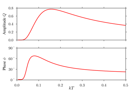
Figure 1: Behaviors of amplitude $Q$ and phase $\phi$ as functions of $kT$, where $m=0.02$, $\gamma m=3.00$, $h=0.20$, and $\Omega=0.04$. Both $Q$ and $\phi$ show their single peaks.

Suggested energy harvesters by the method of SR possess bi-stable potential CRMcinnes2008enhanced ; KNakano2014feasibility ; YZhang2014feasibility . Here is assumed that dynamical equation of the SR harvesters are represented altogether by the following formula:

$$m\frac{{\rm d}\dot{x}}{{\rm d}t}=-m\gamma\dot{x}-\frac{\partial V(x,t)}{\partial x}+R(t),$$ (1)

$$-\frac{\partial V(x,t)}{\partial x}=-\frac{{\rm d}U(x)}{{\rm d}x}+h\cos\Omega t$$

$$\hskip 42.39458pt=-(x^{3}-x)+h\cos\Omega t$$

where $R(t)$ is given as zero-mean white Gaussian noise of auto-correlation function:

$$<R(t)R(t+\Delta t)>=2\gamma mkT\delta(\Delta t).$$ (2)

Where $m$ denotes oscillator mass of a harvester, $x$ displacement, $m\gamma$ damping constant, $h\cos\Omega t$ sinusoidal external force, $U(x)$ bi-stable potential, $k$ Bolztman constant, and $T$ noise temperature. $\dot{(~{})}$ implies time differential ${\rm d}/{\rm d}t$ and $<\,>$ ensemble average operation. We take dissipative energy of controlled motion at frequency $\Omega$ as harvested energy.

Without loss of generality, we can introduce the previously obtained theoretical relationship from RTakahashi2005interaction ; MIDykman1992phase ; LGammaitoni1998stochastic . In particular, $Q$ and $\phi$ are defined in RTakahashi2005interaction and MIDykman1992phase .

$$<x>=Q\cos(\Omega t-\phi)$$ (3)

$$Q=\frac{h}{kT}\frac{W}{\sqrt{W^{2}+\Omega^{2}}}$$ (4)

$$\phi=\arctan{\frac{(\Omega/\Omega_{\rm r})(\Omega_{\rm r}^{2}W+\Omega^{2}kT)}{\Omega_{\rm r}W^{2}+\Omega^{2}kT}}$$ (5)

$$\frac{W}{2}=\frac{\omega_{\rm 0}\omega_{\rm b}}{2\pi\gamma m}\exp\left(-\frac{\Delta U}{kT}\right)$$ (6)

Response of amplitude $Q$ and phase $\phi$ for noise intensity $kT$ are shown in Fig. 1. $\Omega_{\rm r}$ is a relaxation rate defined by ${{\rm d}^{2}U/{\rm d}x^{2}}|_{x=\pm 1}$ MIDykman1992phase . $W/2$ corresponds to Kramers rate LGammaitoni1998stochastic at $\omega_{0}={\rm d}^{2}U/{\rm d}x^{2}|_{x=\pm 1},~{}\omega_{b}={\rm d}^{2}U/{\rm d}x^{2}|_{x=0}$, and potential barrier $\Delta U=1/4$. According to the reaction of $Q$ in Fig. 1, SR appears around $kT=0.1$. When SR appears, the dissipative energy becomes maximum as confirmed in CRMcinnes2008enhanced ; KNakano2014feasibility ; YZhang2014feasibility . The results explain that the external force frequency $\Omega$ matches the time lag to overcome the potential barrier for the harvester.

On the other hand, when a harmonic oscillator has phase lag $\pi/2$ to sinusoidal external force, so called resonance appears, then dissipative energy becomes maximum. Similar phenomena is also confirmed in nonlinear oscillators YSusuki2007ener . In Fig. 1, phase lag $\phi$ becomes maximum at SR MIDykman1992phase . However, it has not been accounted for the relationship between phase lag and dissipative energy.

III Active and reactive power

Here we focus on the relationship of phase lag $\phi$ and energy flow in system of Eqs. (1) and (2). Since there are two external forces; sinusoidal force and noise, it is difficult to decide each contribution. For energy harvesting by SR, it is necessary to see the energy flow. From Eq.(1), the following relationship is obtained.

$$\frac{m}{2}\frac{{\rm d}}{{\rm d}t}<\dot{x}^{2}> = -m\gamma<\dot{x}^{2}>-<\frac{{\rm d}U}{{\rm d}x}\dot{x}>$$ (7)

$$+<\dot{x}>h\cos\Omega t+<R(t)\dot{x}>.$$

Here allocates each term to input, active and reactive power. Through the mechanical-electrical analogy KOgata , electrical voltage and current correspond to externally given mechanical force and the velocity of oscillator, respectively, so that the correspondence of electrical active power to mechanical dissipative power appears. At the same time, the reactive power can be explained as the mechanical energy flow. Generally active and reactive power are averaged over a period. On the other hand, instantaneous input, active, and reactive power are depicted as follows:

Input power:

$$<\dot{x}h\cos\Omega t>+<R(t)\dot{x}>$$

$$\hskip 14.22636pt=-\frac{1}{\gamma m}\left<\frac{\partial V}{\partial x}\right>h\cos\Omega t+\gamma kT,$$ (8)

Active power:

$$<m\gamma\dot{x}^{2}>=\gamma kT+\frac{1}{\gamma m}\left<\frac{\partial V}{\partial x}\right>^{2},$$ (9)

Reactive power:

$$\frac{m}{2}\frac{{\rm d}}{{\rm d}t}<\dot{x}^{2}>+\left<\frac{{\rm d}U}{{\rm d}x}\dot{x}\right>$$

$$\hskip 14.22636pt=-\frac{1}{\gamma m}\left<\frac{{\partial}V}{{\partial}x}\right>^{2}-\frac{1}{\gamma m}\left<\frac{{\partial}V}{{\partial}x}\right>h\cos\Omega t,$$ (10)

where the following two equations derived from the Fokker-Plank equation are substituted into Eq.(7).

$$<\dot{x}^{2}>=\frac{kT}{m}+\frac{1}{\gamma^{2}m^{2}}\left<\frac{\partial V}{\partial x}\right>^{2}$$ (11)

$$<\dot{x}>=-\frac{1}{\gamma m}\left<\frac{\partial V}{\partial x}\right>.$$ (12)

In Eqs.(8), (9), and (10), those power are consisted of following $P_{\rm i}~{}({\rm i}=1,2,3)$:

$$\hskip 2.84526ptP_{1}=-\frac{1}{\gamma m}\left<\frac{\partial V}{\partial x}\right>h\cos\Omega t,~{}~{}~{}P_{2}=\frac{1}{\gamma m}\left<\frac{\partial V}{\partial x}\right>^{2},~{}~{}~{}P_{3}=\gamma kT.$$

Here we average $P_{\rm i}~{}({\rm i}=1,2,3)$ over a period $2\pi/\Omega$, and express them as $\overline{P_{\rm i}}~{}({\rm i}=1,2,3)$. Fig. 2 shows them as functions of noise strength $kT$. $\overline{P_{3}}$ is in proportion to $kT$. $\overline{P_{1}}$ and $\overline{P_{2}}$ reach thier peak around SR.

Here we discuss the physical meaning of $P_{\rm i}~{}({\rm i}=1,2,3)$. The power sources of $P_{1}$ and $P_{3}$ are obvious. $P_{1}$ is input power from sinusoidai force $h\cos\Omega t$, because $<\dot{x}h\cos\Omega t>=P_{1}$ can be derived from Eq.(12). $P_{3}$ is input power from noise $R(t)$, because $<R(t)\dot{x}>=P_{3}$ can be derived from Eqs.(1) and (2). $P_{3}$ corresponds to dissipative power consumed by localized small scale vibration. On the other hand, $P_{2}$ can not be derived directly from the given forces, and the power source is not clearly defined. As you can understand, $P_{2}$ is a term which cancels out by adding both active (Eq.(9)) and reactive powers (Eq.(10)). However, at first, $P_{2}$ includes frequency $\Omega$, since $P_{2}$ depends on potential shape $V(x,t)$, as in Eqs.(1) and (3). In addition, $P_{2}$ becomes maximum around SR as shown in Fig. 2. Therefore $P_{2}$ seems a power to vibrate over the potential barrier periodically.

Next, energy flow is discussed based on the above power allocation. The input power $P_{3}$ from noise goes directly to active power and is consumed. Fig. 2 and Eqs.(8), (9), (10) leads that, when SR appears, $P_{1}$ contributes to the reactive power mostly. Then $P_{2}$ increases, since reactive power ($=-P_{2}+P_{1}$) of Eq.(10) has a limit. Consequently active power $P_{2}$ including $\Omega$ also increases. And $P_{2}$ equals to the dissipative power of controlled motion. The special feature is that, when SR appears, phase lag $\phi$ and also $P_{2}$ are maximized at an appropriate noise intensity. Hence, it is reasonable to adjust dissipative power by altering $kT$ similar to power factor correction in a circuit.

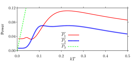
Figure 2: $\overline{P_{1}}$ (red solid line), $\overline{P_{2}}$ (blue dotted line), $\overline{P_{3}}$ (green broken line) as a function of $kT$ calculated theoretically.

IV Numerical estimation

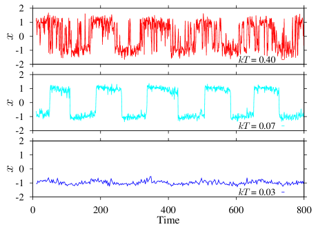
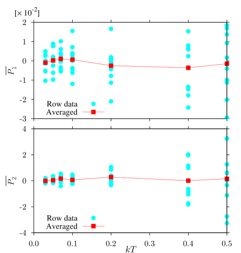
Figure 3: Time changes of displacement $x$ under the noise intensity $kT=0.03,0.07,0.40$ with $h$ and $\Omega$ kept constant.

Figure 4: Numerically estimated $\overline{P_{1}}$ and $\overline{P_{2}}$ under different noise strength.

Figure 4 shows time dependence of displacement $x$ at $kT=0.03$, $0.07$, and $0.40$. SR appears around $kT=0.07$. Fig. 4 shows numerically calculated $\overline{P_{1}},\overline{P_{2}}$ from Eqs.(1) and (2). Blue (gray) bullets at each $kT$ are values of ten trials, and red (black) squares are ensenble averaged value from the ten trials. $\overline{P_{1}}$ and $\overline{P_{2}}$ become maximum locally around $kT=0.07$ where SR appears. However the peaks are not clear as in Fig. 2. $\overline{P_{2}}$ increases at $kT=0.5$. This is because of a reduction in calculation accuracy as we can see that the variance of blue (gray) bullets increases with noise intensity $kT$ growth.

V Conclusion

In this letter, SR is investigated as a method for energy harvesting from noise. When SR appears, the phase lag and dissipative power of frequency $\Omega$ are maximized at an appropriate noise intensity. The result suggests the possibility of maximizing dissipative energy of controlled motion as same as the analogous to power factor correction.

Acknowledgement

We acknowledge fruitful discussions with Edmon Perkins, visiting researcher supported by NSF-JSPS program. This work is supported in part by Grant-in-Aid Challenging Exploratory Research No. 26630176. MK is financially supported by Kyoto University graduate school of engineering.

References

- (1) R. P. Feynman, R. B. Leighton, and M. L. Sands, The Feynman lectures on physics: Mainly mechanics, radiation, and heat, vol.I, The New Millennium Edition, (Basic Books, 2011), Chap.46.
- (2) T. R. Kelly, H. D. Silva, and R.A. Silva, Nature, 401, no.6749, pp.150–152, (1999)
- (3) C. McInnes, D. Gorman, and M. Cartmell, J Sound Vib, 318, no.4, pp.655–662, (2008).
- (4) K. Nakano, M.P. Cartmell, H. Hu, and R. Zheng, Stroj vestn-j Mech E , 60 no.5, pp.314–320, (2014).
- (5) Y. Zhang, R. Zheng, and K. Nakano, JPCS, p.012097, IOP Publishing, (2014).
- (6) R. Benzi, A. Sutera, and A. Vulpiani, J Phys A-math gen, 14 no.11, p.L453, (1981).
- (7) C. Nicolis and G. Nicolis, Tellus, 33 no.3, pp.225–234, (1981).
- (8) J. K. Douglass, L. A. Wilkens, E. Pantazelou, and F. Moss, Nature, 365 no.6444, pp.337–340, (1993).
- (9) D. F. Russell, L. A. Wilkens, and F. Moss, Nature, 402 no.6759, pp.291–294, (1999).
- (10) Y. Kurita, M. Shinohara, and J. Ueda, Human-Machine Systems, IEEE Trans. on, 43 no.3, pp.333–337, (2013).
- (11) V. Rallabandi and P.K. Roy, Magn reson imaging, 28, no.9, pp.1361–1373, (2010).
- (12) T. Oya, T. Asai, R. Kagata, S. Kasai, and Y. Amemiya, Int Congr Ser, pp.213–216, (2006).
- (13) S. Kasai, Y. Shiratori, K. Miura, Y. Nakano, and T. Muramatsu, phys status solidi (c), 8, no.2, pp.384–386, (2011).
- (14) R. Takahashi and M. Suzuki, Physica A, 353, pp.85–100, (2005).
- (15) M. I. Dykman, R. Mannella, P. V. E. McClintock, and N. Stocks, PRL, 68, no.20, p.2985, (1992).
- (16) L. Gammaitoni, P. Hänggi, P. Jung, and F. Marchesoni, Rev mod phys, 70, no.1, p.223, (1998).
- (17) Y. Susuki, Y. Yokoi, and T. Hikihara, CHAOS, 17, no.2, p.023108, (2007).
- (18) K. Ogata, System Dynamics, 2nd ed. Prentice Hall, (New Jersey, 1992) Chap.4.