Unwinding the hairball graph: pruning algorithms for
weighted complex networks

Abstract

Empirical networks of weighted dyadic relations often contain “noisy” edges that alter the global characteristics of the network and obfuscate the most important structures therein. Graph pruning is the process of identifying the most significant edges according to a generative null model, and extracting the subgraph consisting of those edges. Here, we focus on integer-weighted graphs commonly arising when weights count the occurrences of an “event” relating the nodes. We introduce a simple and intuitive null model related to the configuration model of network generation, and derive two significance filters from it: the Marginal Likelihood Filter (MLF) and the Global Likelihood Filter (GLF). The former is a fast algorithm assigning a significance score to each edge based on the marginal distribution of edge weights whereas the latter is an ensemble approach which takes into account the correlations among edges. We apply these filters to the network of air traffic volume between US airports and recover a geographically faithful representation of the graph. Furthermore, compared with thresholding based on edge weight, we show that our filters extract a larger and significantly sparser giant component.

I Introduction

Graphs or networks are widely used as representations of the structure and dynamics of complex systems strogatz_exploring_2001 ; albert_statistical_2002 ; barthelemy_spatial_2011 ; jin_structure_2001 ; newman_structure_2003 . Too often in practice, networks of observed dyadic relationships are too dense to be of immediate use: the topology of the network is dominated by an abundance of “noisy” edges that must somehow be removed before the most significant structures are revealed. This process—which we refer to as pruning—is particularly useful in visualizing the so-called “hairball” networks, and can conceivably enhance the efficacy of community detection methods by serving as a preconditioner.

We distinguish between the problem of pruning discussed here on the one hand, and the problem of sparsification on the other. Sparsification is the problem of approximating a network using a subgraph with fewer edges such that some property of the graph is preserved within a desired tolerance. The goal of sparsification is typically to compute network characteristics of the original graph, only at a lower computational cost. Therefore, one must aim to minimally alter the character of the network in the process. For instance, when faced with a dense similarity matrix derived from a large number of data points, it is desirable to work instead with a sparse subgraph with the same community structure as the full graph. For such applications, one may use sparsifiers using random spanning trees goyal_expanders_2009 ; kelner_faster_2009 ; wilson_generating_1996 , or others that explicitly approximate the spectral properties of the graph Laplacian spielman_spectral_2008 .

The problem of pruning on the other hand, involves the removal of a possibly large number of spurious edges that are believed to obfuscate an unknown core that contains the most important structures. It is therefore implied that the coveted core is different from the observed, noisy graph. The properties of the core such as its community structure are not known a priori, and thus, it is not clear which graph properties if any should be preserved in the process. In fact, the goal should arguably be to alter important features of the graph until the properties of the hidden core are revealed.

Graph pruning is most commonly done by thresholding based on edge weights. This approach equates significance with edge weight, and fails to take into account the relationship between the edge, its incident vertices and their other edges. Therefore, thresholding based on weight systematically discounts low-degree vertices and structures they represent. In order to address this issue, alternative methods have been proposed such as the filters of serrano_extracting_2009 and radicchi_information_2011 . These methods consist of assigning a p-value to each edge based on a null model of edge weight distribution, and subsequently filtering out all but those edges least likely to have occurred due to pure chance, namely those with the smallest p-values. The disparity filter of serrano_extracting_2009 accomplishes this by evaluating all edges incident on a given vertex in relation to one another. The GloSS filter of radicchi_information_2011 is a computationally involved method attempting to preserve the weight distribution of edges. Here we propose two new measures of significance based on a different null model. The first, which we dub “Marginal Likelihood Filter” (MLF) is a local significance measure computed independently for each edge from the marginal probability distribution of each edge weight, reducing pruning to a sorting problem. We judge the significance of an edge in relation to the properties of both of its end vertices. According to our null model, the higher the degrees of two arbitrary vertices, the more likely they are to be connected to one another by chance. Therefore, the higher the degrees of an edge’s incident vertices, the larger its weight must be for it to be considered significant. The second, called the “Global Likelihood Filter” (GLF) is a global measure computed for each possible subgraph of a given size “as a whole”, thus taking into account the correlation among edges. Pruning then consists of finding the subgraph with the highest significance. While arguably the more principled approach due to its global nature, GLF requires the use of Monte Carlo methods and can thus become prohibitively expensive for large graphs. MLF, on the other hand, provides a fast (almost linear in the number of edges) method easily scalable to very large graphs.

In the following sections we will define the null model and derive from it the marginal likelihood edge filter for undirected as well as directed weighted networks. Then we show how, from the same null model, an ensemble approach to pruning can be developed and we describe the resulting filter (GLF). We apply the methodology to the network of air traffic volume between US airports in 2012, and demonstrate how the filtered subgraphs differ in important topological measures from those obtained from simple weight thresholding at a comparable level.

II Marginal likelihood filter

The null model defines a “random” ensemble of graphs resembling the realized graph. We must therefore select some attributes of our graph and demand that the random ensemble possess those attributes. We propose a null model that preserves the total weight of the realized graph and its degree sequence on average. Here, by the degree of a vertex we mean the sum of the weights of all its incident edges—also known as the node’s strength—and we assume all weights to be positive integers. Further, we conceive of a weighted edge as multiple edges of unit weight.

For a weighted undirected graph then, our null model assumes that the unit edges of the graph are assigned to a pair of vertices, one at a time, and independently of one another. For each edge, the two end points are chosen independently at random with probabilities proportional to the degrees. That is, a vertex with a higher realized degree is proportionally more likely to be assigned to an edge than a vertex of lower degree. This leads to the same pair-wise connection probability predicted by the configuration model newman_structure_2003 in the sparse or classical limit park_statistical_2004 . Intuitively, vertices $i,j,\cdots$ in this model behave like chemical reactants in a solution with concentrations $k_{i},k_{j},\dots,$ whose pairwise reaction rates are proportional to both reactant concentrations. Given this null model, for any arbitrary pair of vertices $i$ and $j$ with degrees $k_{i}$ and $k_{j}$, we can compute the probability mass function of the weight of the edge connecting them.

Suppose the graph possesses a total of $T$ edges (recall that we count a weighted edge as multiple edges of unit weight). Throughout, we will assume that $T\gg 1.$ Each unit edge must choose two incident vertices at random, with probabilities proportional to vertex degrees. The probability that $m$ out of the $T$ edges will choose nodes $i$ and $j$ as their end points is given by the binomial distribution $B(T,p).$ In short, the null model is defined by the following distribution for the weight $\sigma_{ij}$ of the $(i,j)$ pair:

$$\Pr\left[\sigma_{ij}=m\,|\,k_{i},k_{j},T\right] = {T\choose m}p^{m}(1-p)^{T-m}$$ (1)

$$\mbox{where}\,\,\,p=\frac{k_{i}k_{j}}{2T^{2}}, T=\frac{1}{2}\sum_{i}k_{i}$$ (2)

One can verify that the expected value of the degree of node $i$ is $\sum_{j}k_{i}k_{j}/(2T)=k_{i}.$ Thus, the ensemble defined by the null model preserves the degree sequence on average. We note that depending on the value of $pT,$ for large $T$ this distribution can tend to Poisson or normal distribution. With this distribution at hand, we can proceed to compute a p-value for the realized value of the edge weight connecting $i,j.$ Denote the realized weight of the $(i,j)$ edge by $w_{ij}.$ Then, we can define the p-value as

$$s_{ij}(w_{ij})=\sum_{m\geq w_{ij}}\Pr\left[\sigma_{ij}=m\,|\,k_{i},k_{j},T\right].$$ (3)

This definition corresponds to a so-called one-tailed test where higher weights are considered more extreme regardless of the expected value of the null distribution. Once we have computed the p-value for all edges, we can proceed to filter out any edge with p-value $s_{ij}(w_{ij})<\alpha$ for any threshold $\alpha$ of our choosing. This will retain the edges least likely to have occurred purely by “chance” according to the marginal distributions resulting from the null model. Numerical evaluation of the p-value from the binomial probability distribution will pose challenges due to the large factorials involved. For large $T,$ one can use asymptotic approximations of the binomial distribution instead (Poisson for $pT=O(1)$ and normal for $pT$$\gg 1$). Some standard statistics packages include implementations of the so-called binomial test which computes precisely the p-value in question. We use the implementation in Python’s statsmodels package.

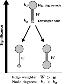
(a)

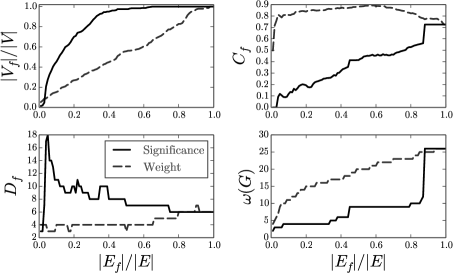
(b)

(c)

Figure 1: (a) Qualitative schematic of the partial order defined by the MLF filter: three pairs of nodes connected by edges of varying weights. The size of a node represents its (weighted) degree and the thickness of the edge represents its integer weight. The top case has a higher significance than either of the bottom cases: with the node degrees fixed, a higher edge weight $W$ results in higher significance. With the weight $W$ fixed, lowering either end-node’s degree results in higher significance. (b) Four graph measures computed for the US air traffic network (2012) filtered at different levels using the Marginal Likelihood Filter (solid) and weight thresholding (dashed). The $x$ axis is the proportion of edges retained by the filtering. Clockwise from top left: 1- Proportion of nodes in the giant component. 2- Clustering coefficient for the giant component. 3- Diameter of the graph. 4- Clique number of the graph. (c) The Jaccard similarity between the set of “on edges” produced by the MLF and GLF filters.

We can generalize this formalism to the case of weighted directed graphs. Here, the graph is characterized by two degree sequences: the in-degree sequence, and the out-degree sequence. For a directed edge between vertices $i,j$, the realized state consists of

$$\sigma_{ij}\,\,\mbox{weight of the directed edge }(i,j)$$ (4)

$$k_{i}^{out}\mbox{ out-degree of node }i$$ (5)

$$k_{j}^{in}\mbox{ \,\ in-degree of node $j$}$$ (6)

Again, we assume as the null model, that each of the $T$ directed edges must choose a source vertex and a target vertex independently at random, such that both the in-degree distribution and the out-degree distribution reflect the realized values on average. Thus, the source and target vertices must be chosen with probability proportional to the nodes’ out and in-degrees respectively. The weights will be distributed binomially:

$$\Pr\left[\sigma_{ij}=m\,|\,k_{i}^{out},k_{j}^{in},T\right] = {T\choose m}p_{ij}^{m}(1-p_{ij})^{T-m}$$ (7)

$$\mbox{where}\,\,\,p_{ij}=\frac{k_{i}^{out}k_{j}^{in}}{T^{2}}, T=\sum_{i}k_{i}^{out}$$ (8)

The p-value is defined just as in $\left(\ref{eq:pvalue}\right),$ replacing $k_{i}$ with $k_{i}^{out}$ and $k_{j}$ with $k_{j}^{in}.$

II.1 Excluding self-edges

The connectivity probability $\left(\ref{eq:pij-main}\right)$ used in our null model corresponds to the configuration model (more specifically, its sparse limit park_statistical_2004 ) in which self-edges are not precluded. In most applications, whether the observed network contains self-edges or not, this poses no problem in principle since randomization necessarily involves forgetting certain properties of the observed instance. Furthermore, the sparse limit of the configuration model is a good approximation of the special loopless case when no vertex is dominant in terms of weighted degree. However, if the preclusion of loops is fundamental to the underlying dynamics or structure of the graph, one can easily modify the null model to account for this fact. We find an alternative expression for the connectivity probability $p_{ij}$ by seeking solutions of the form

$$p_{ij}=\begin{cases}f(k_{i})f(k_{j})&i\neq j\\ 0&i=j\end{cases}$$ (9)

such that the degree sequence is preserved on average:

$$k_{i}=T\sum_{j\neq i}p_{ij}=Tf(k_{i})\left(\sum_{j}f(k_{j})-f(k_{i})\right).$$ (10)

The difference here is that $i$ is excluded from the sum. Note that this equation automatically satisfies the loopless normalization condition $\sum_{i<j}p_{ij}=1$ as well. To first order in $f(i)/\sum f(i),$ the solution is $f(i)=k_{i}/T\sqrt{2}$ and we recover $\left(\ref{eq:pij-main}\right).$ One can continue solving for higher order terms to compute the loopless solution to arbitrary precision. Here we demonstrate the solution of the second order term. Writing $f(k_{i})=f_{i}+\delta_{i}+O\left(\left(k_{i}/T\right)^{3}\right)$ where $f_{i}=k_{i}/T\sqrt{2}$ is the first order solution, and solving for $\delta_{i}$ to second order, we find

$$\delta_{i}=\frac{f_{i}^{2}-cf_{i}}{\sqrt{2}}\,\,\,\mbox{where}\,\,\,c=\sum_{j}\delta_{j}.$$ (11)

We need only solve for $c$ by summing over all $\delta_{i},$ which yields

$$c=\frac{1}{\left(1+\sqrt{2}\right)}\sum_{i}f_{i}^{2}.$$ (12)

We will continue to refer to the simplified model defined by $\left(\ref{eq:pij-main}\right)$ as the MLF, and to the modified versions defined by (10), (11) and (12) as the second order loopless MLF.

III Global likelihood filter

The Marginal Likelihood Filter described above assigns a p-value independently to each edge allowing us to define the pruned graph simply as the subgraph consisting of the top most significant edges. This results in a fast algorithm running in $O(\left|E\right|\log\left|E\right|)$ time where $|E|$ is the size of the edge set of the graph. However, this comes at a cost: it is assumed that the statistical significance of an edge is independent of the presence of other edges. In this section we develop an ensemble approach to pruning that avoids this assumption. In order to motivate this approach, we begin by reviewing the exponential random graph model.

The so-called exponential random graph model (ERGM) has been used for decades—especially in the social sciences—to model unweighted empirical networks and study the relationship between different graph properties where simpler regression models fail due to the correlated nature of the data. The model consists of a probability measure on the set of all possible graphs with $n$ vertices given by

$$P(G)\sim e^{\theta_{1}x_{1}(G)+\theta_{2}x_{2}(G)+\cdots\theta_{m}x_{m}(G)}$$ (13)

where $x_{i}(G)$ is some graph property such as the total number of edges or the degree of a specific node, etc., and $\theta_{i}$ is a parameter that must be adjusted such that $\left\langle x_{i}(G)\right\rangle$, the ensemble average of property $x_{i}$, matches the observed value. It was shown park_statistical_2004 that this probability measure can be derived as the Boltzmann (or Gibbs) distribution for a canonical ensemble of graphs. In other words, this is the probability measure that maximizes the entropy while keeping each graph property $x_{i}$ equal to a fixed value on average, just as the familiar Boltzmann distribution of the canonical ensemble in statistical mechanics yields a maximum entropy ensemble with a given average energy. The parameter $\theta_{i}$ then acts as an inverse temperature whose value adjusts $\left\langle x_{i}(G)\right\rangle.$ Given one such model, one can compute other graph properties of interest as derivatives of the partition function.

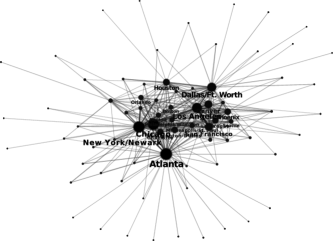
(a)

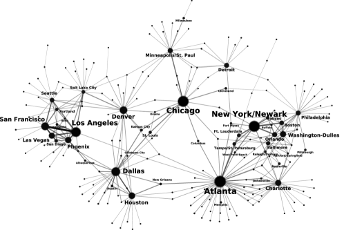
(b)

Figure 2: Visualizations of the US airport transportation network (2012) pruned using (a) weight thresholding, and (b) the Marginal Likelihood Filter. In each case, the top 15% of the edges with the respective edge attribute are retained. Both plots are rendered using the same standard Fruchterman-Reingold layout algorithm with identical parameters.

More recently, the ERGM was generalized to weighted or multi-edge graphs sagarra_configuration_2014 ; sagarra_statistical_2013 where a weighted edge/multi-edge represents the number of “events” associated with a pair of nodes. Examples include transportation traffic volume networks where the weight of the edge between two cities counts the number of “travel events” between the two cities over a given time period. Here, a pair of nodes can be viewed as a physical state that can be occupied by an arbitrary number of particles, and the weight of their incident edge corresponds to the occupation number of the state. The crucial difference here is the distinguishability of the events as pointed out by sagarra_statistical_2013 . Unlike physical particles, macroscopic events represented by multi-edge graphs are distinguishable, and thus, the statistics resemble a Boltzmann gas rather than a Bose-Einstein gas huang_introduction_2001 . In concrete terms, this manifests as a multiplicity number associated to each weighted graph configuration that must be taken into account in the partition function.

Let us now define the GLF filtering procedure. Suppose we have an observed graph $G_{0}$ with $n$ vertices and edge weights $w_{ij}\in\{0,1,2,\cdots\}$ for $i,j=1,2,\cdots,n$ so that the graph possesses $m$ weighted edges (edges with positive weight). As the null model, we consider the maximum entropy ensemble $\mathscr{G}$ of (integer) weighted graphs with $n$ vertices such that the degree sequence is equal to that of the observed graph on average. This automatically ensures that the total edge strength of the graph is also equal to that of the observed graph on average. Thus, following park_statistical_2004 and sagarra_statistical_2013 , we obtain the grand canonical ensemble defined by the Boltzmann distribution

$$P(G)=\frac{1}{Z}g\left[\left\{\sigma_{ij}\right\}\right]\exp\left[-\sum_{i<j}(\theta_{i}+\theta_{j})\sigma_{ij}\right]\,\,\,\forall G\in\mathscr{G}$$ (14)

where $\sigma_{ij}\in\{0,1,2,\cdots\}$ is the weight of the $(i,j)$ edge in $G$, $\theta_{i}$ is the inverse temperature determining $\left\langle k_{i}\right\rangle$, and

$$g\left[\left\{\sigma_{ij}\right\}\right]=\frac{\left(\sum_{i<j}\sigma_{ij}\right)!}{\prod_{i<j}\sigma_{ij}!}$$ (15)

is the multiplicity of the configuration $\left\{\sigma_{ij}\right\}$ resulting from the distinguishability of the events. Note that using the partition function $Z,$ we can compute the parameters $\theta_{i}$ such that the ensemble’s expected value of the total weight and the degree sequence match those of the observed graph, namely $T=\frac{1}{2}\sum_{ij}w_{ij}$ and $\left\{k_{i}\right\}$. In the thermodynamic limit $T\gg 1,$ up to an additive constant, the log-likelihood is given by

$$\log P(G)=\log\left(\overline{N}!\right)+\sum_{i<j}\left[\sigma_{ij}\log p_{ij}-\log\left(\sigma_{ij}!\right)\right]$$ (16)

where

$$p_{ij}=\frac{k_{i}k_{j}}{2T^{2}},\,\,\,\overline{N}=\sum_{i<j}\sigma_{ij}.$$ (17)

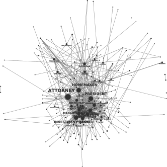
(a)

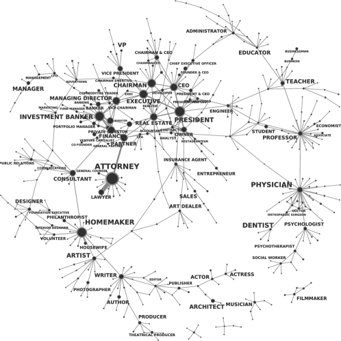
(b)

Figure 3: Visualizations of the network of interdependent occupations in the state of New York, pruned using (a) weight thresholding, and (b) the Marginal Likelihood Filter. Both are truncated at the 3% level and plotted using a standard Fruchterman-Reingold layout algorithm with identical parameters.

To evaluate the large factorials involved, one can use the highly accurate Stirling approximation. For the details of the computations leading to $\left(\ref{eq:logP},\ref{eq:pij}\right)$, see Appendix A.

We posit that the most significant subgraph with $m^{\prime}<m$ edges is the minimum likelihood subgraph among the set of all subgraphs of $G_{0}$ possessing $m^{\prime}$ non-zero weights, according to the null distribution $\left(\ref{eq:ensemble distribution}\right)$. This is the subgraph least likely to have been generated purely by chance given the null distribution. Note that unlike the Marginal Likelihood Filter discussed in the previous section, here we cannot assign independent scores to edges and select the top $m^{\prime}.$ The term $\log(\overline{N}!)$ combines the effect of all existing edges in a realization inseparably. Therefore, solving this minimum likelihood problem requires a standard Monte Carlo simulation. For instance, a Metropolis algorithm can be used where initially a random set of $m^{\prime}<m$ edges from $G_{0}$ are “turned on”, and then at each step, one of the “on” edges is chosen at random and replaced with a randomly selected “off” edge. The change is accepted if it decreases $\log P(G)$ and rejected with probability $1-\exp(-\Delta\log P(G))$ otherwise, all the while keeping track of the minimum likelihood set found thus far. The change in log-likelihood is easy to compute since the second term in $\left(\ref{eq:logP}\right)$ is a sum over all “on edges”, and $\Delta\log\left(\overline{N}!\right)$ can also be computed easily using the Stirling approximation.

IV Application to real world networks

In this section, we apply weight thresholding and the Marginal Likelihood Filter to two networks. The first is the network of US air traffic in 2012 (data courtesy of Alessandro Vespignani, following the work in barrat_architecture_2004 .) In this network each node is a US city and an edge weight represents the air traffic volume between airport(s) in one city and another, aggregated over the year 2012. The network is symmetrized and undirected.

Fig. 1(b) summarizes four graph measures computed for this network truncated at different levels, both using the MLF and using weight thresholding. The GLF filter yields results similar to the MLF. The $x$ axis is the percentage of the total edges retained in the truncated version. The four measures are the following: 1. the size (number of nodes) remaining in the giant component $(\mbox{$|V_{f}|/|V|$}$) 2. the averaged local clustering for the giant component $C_{f}$ newman_structure_2003 . 3. the diameter of the graph $D_{f}$ 4. the clique number of the graph $\omega(G)$ which measures the size of the largest complete subgraph, or clique, found within the graph west_introduction_2001 . We observe that at the same level of truncation, the significance filter leads to a much larger giant component. Roughly at the 50% level, almost all nodes are already in the giant component. When pruning highly connected graphs, retaining a large giant component is naturally desirable since decomposing the graph into a large number of small components results in the loss of all connectivity information (e.g. network distance) between most pairs of nodes. Even if one hopes to accentuate the community structure of the graph via pruning, it is still preferable for the communities to remain connected to the giant component via weak links than to be completely cut off as distinct connected components. The clustering coefficient for the weight-threshold truncations remains roughly the same for all thresholds, whereas the significance filter produces considerably lower clusterings at severe truncations, suggesting that the truncated graph is rather sparse. The diameter (longest shortest path) of the truncated graphs are also significantly different between the two filters, with the significance filter yielding rather large diameters at severe truncations, suggesting a sharper departure from a fully connected graph. Finally, we observe a significant difference between the clique numbers of the graphs according to the two filters. For the weight filter, $\omega$ increases steadily as more and more edges are included, whereas for the significance filter, it remains at a more or less constant and low value until about the 90% threshold at which point a sharp increase brings it to the level of the untruncated network. This reinforces the finding on the clustering number suggesting that the significance threshold produces graphs with lower local densities.

Fig. 2 compares the US airport transportation network truncated using the MLF and weight thresholding. (Again, the GLF produces results very similar to the MLF.) In both cases 15% of the edges are retained and the plots are rendered using a generic force-directed layout algorithm (Fruchterman-Reingold) with identical parameters. While the weight thresholded graph still appears as a “hairball” graph, the significance-filtered graph naturally unfolds into what resembles the actual geographical distribution of the nodes almost perfectly. This particular effect is in part due to the removal of long-range high-volume edges that are nevertheless assigned a low significance due to the high strength of their incident vertices. For instance, the edges (Los Angeles, New York City) and (Chicago, San Francisco) are absent from this truncation despite their large weight. Our filter is thus prioritizing local connections over long-range connections indicating the higher importance of these links with respect to the overall traffic volume of their two end points. This is of course specific to this network, but demonstrates that some underlying property of the network is revealed by pruning. Finally, Fig. 1(c) compares the edge sets selected by the MLF and GLF filters ($E_{MLF},E_{GLF})$ at different truncation levels. The $y$ axis is the Jaccard similarity between the two edge sets defined as

$$J(A,B)\equiv\frac{\left|A\cap B\right|}{\left|A\cup B\right|}.$$ (18)

We observe that the two filters show a high level of similarity—over 80% for truncation thresholds as low as 20%. The disparity is of course to be expected, since in the MLF scheme, the edge set at a lower threshold is necessarily a subset of the edge set at a higher threshold whereas in the GLF scheme, it is possible that an edge which was absent at a higher threshold will be present at a lower threshold (more severe truncation).

We also applied the second order loopless MLF to the air traffic network, and found that the pruned graph is virtually indistinguishable from that obtained from the first order (standard) MLF. To be specific, the two pruned graphs differed on a handful of edges. Most notably, the Chicago-Minneapolis and Columbus-Atlanta edges were absent from the result of the loopless MLF, but barely changed the graph layout, suggesting that the standard MLF can serve as a good approximation to the loopless case as well.

Next we applied the MLF to the network of interdependent occupations in the state of New York derived from the database of campaign contributions published by the Federal Election Commission (FEC). This database contains every monetary contribution over $200 by an individual to a federal US election campaign since 1979. Among other information, each record contains the occupation and employer of the donor at the time of the transaction. The author has compiled a “disambiguated” version of this database (to be published separately in the near future), meaning one in which all transactions from the same individual are linked. This database consists of roughly 24,000,000 records from around 6,000,000 individual. Using this disambiguated database one can produce a co-occurrence network of occupations where each node is a distinct occupation label and two labels are linked if both appear in an individual’s history. Thus, an edge can indicate either semantic equivalence (“Doctor” and “Physician”) or a plausible transition (“Postdoc” to “Professor”). The weight of an edge counts the number of times the two end-nodes co-occurred in histories of individuals. For instance, “Lawyer” and “Attorney” are linked with a rather large weight. Similarly, “President” and “CEO” are strongly linked. Due to the large size of the database however, many apparently unrelated occupations are also linked, albeit with lower weights, e.g., a “Doctor” who at some other time identifies as a “Writer”. We can now ask if we can uncover the structure of interrelated occupations by pruning the dense co-occurrence network. Figure 3 shows this network pruned using weight thresholding and the MLF. In both cases, the top 3% of the edges are retained. As with the air transportation network, weight thresholding does little to reveal the important structures within the network while the MLF untangles the network into clearly visible clusters: legal professions are connected through “Partner” to the large cluster of top management occupations, “Homemaker” is in a distinct cluster together with creative and philanthropic occupations, and medical and academic occupations are each in their own clusters.

V Discussion

In order to extract the most significant substructures in a complex network, we have proposed a generative null model, and studied two edge filters resulting from this model. Our significance measures are derived from a null model that preserves the total edge strength and the weighted degree sequence of the graph on average. Simply put, this null model states that if everything were random, two arbitrary vertices would be connected with probability proportional to both their weighted degrees (strengths). In the first filter, the degree of deviation from this null model in the observed network at the edge level, expressed as a p-value, defines the marginal significance of an edge. When applied to real-world networks, this filter extracts subgraphs that are significantly sparser (as measured by clustering, clique number and shortest path length) than one would obtain from simple weight thresholding at the same level, even though it yields higher global connectivity as reflected by the size of the giant component. In the second filter, the likelihood of the occurrence of each subgraph as a whole determines its global significance, and the most significant subgraph corresponds to the minimum likelihood subgraph. Visual inspection of the US airport transportation network filtered using our significance measures reveals how low-weight regional links are prioritized over high-weight long-range links such that the original “hairball” network unfolds into a rather flat graph closely reflecting the actual geographical distribution of the nodes.

Regarding the relationship between the two filters, one more point merits discussion. First, equations $\left(\ref{eq:general-connectivity}\right)$ and $\left(\ref{eq:GLF-nonlinear-system}\right)$ are equivalent. Furthermore, the Gibbs distribution found in $\left(\ref{eq:GLF-multinomial-dist}\right)$ is simply a multinomial distribution when the total edge weight is constrained. It is a standard result that when the joint distribution of multiple variables is multinomial, the marginal distribution of each variable is simply binomial. We see then, that the edge weight distribution used in MLF is simply the marginal distribution of the Gibbs distribution used in GLF.

Let us also emphasize the fact that unlike in sparsification, the goal in pruning is to reveal unknown structures which are obscured by noise. This is why the problem of pruning is not an approximation problem as there are no objective measures of success. Therefore, the merits of a pruning filter such as ours can only be judged by the assumptions defining the null model. A central concern is the balance between over and under-determination. The null model should sufficiently reflect the essential features of the observed graph through its defining constraints. However, one must avoid imposing too many constraints or else the null model will be incapable of accounting for the natural variations in the (unknown) ensemble from which the observed graph is obtained. In this context, our filter can be viewed as a middle ground between the disparity filter serrano_extracting_2009 which defines the null model only based on a node’s incident edges, and the GloSS filter of radicchi_information_2011 which preserves the global distribution of edge weights.

Finally, we outline a number of potential future directions. For highly skewed degree distributions, the asymptotic expansions of different equations in $\left(\ref{eq:general-connectivity}\right)$ may need to be truncated at different orders depending on $k_{i}/T$ in order to produce balanced solutions. Another remaining question is whether one can define an optimal significance threshold for pruning a given graph. Presumably, some combination of the graph measures discussed in fig. 1b as well as other relevant measures can aid the practitioner in determining the appropriate truncation level. However, whether or not a generically applicable recipe can be defined remains to be seen.

Appendix A  

In this appendix, we will compute the partition function for the ensemble defined by $\left(\ref{eq:ensemble distribution}\right)$ and enforce the constraints on the degree sequence by solving for the parameters $\theta_{i},\,i=1,2,\cdots,n.$ The partition function is defined by

$$Z = \sum_{\left\{\sigma_{ij}\right\}}g\left[\left\{\sigma_{ij}\right\}\right]\exp\left[-\sum_{i<j}(\theta_{i}+\theta_{j})\sigma_{ij}\right]$$ (19)

$$= \sum_{N=0}^{\infty}\sum_{\begin{subarray}{c}\left\{\sigma_{ij}\right\}\\ \sum\sigma_{ij}=N\end{subarray}}N!\prod_{i<j}\dfrac{1}{\sigma_{ij}!}e^{-(\theta_{i}+\theta_{j})\sigma_{ij}}.$$ (20)

Using the Multinomial theorem, the inner sum simplifies:

$$Z = \sum_{N=0}^{\infty}\left(\sum_{i<j}e^{-(\theta_{i}+\theta_{j})}\right)^{N}$$ (21)

$$= \frac{1}{1-\sum_{i<j}e^{-(\theta_{i}+\theta_{j})}}.$$ (22)

The expected values of the degrees can be computed as follows:

$$\left\langle\sum_{j\neq i}\sigma_{ij}\right\rangle=-\frac{\partial}{\partial\theta_{i}}\log Z$$ (23)

Setting these equal to the $k_{i}$ respectively and defining

$$x_{i} \equiv e^{-\theta_{i}}\,\,i=1,2,\cdots,n$$ (24)

after rearranging the terms we obtain

$$k_{i} =\frac{x_{i}\sum_{j\neq i}x_{j}}{1-\sum_{i<j}x_{i}x_{j}}$$ (25)

$$\sum k_{i} =2T$$ (26)

Summing the first equation over $i$ and using the second equation yields $\sum_{i<j}x_{i}x_{j}=T/(1+T).$ Thus we obtain a system of $n$ nonlinear equations

$$\frac{k_{i}}{1+T}=x_{i}\left(\sum_{j=1}^{n}x_{j}-x_{i}\right)\,\,\,i=1,2,\cdots,n.$$ (27)

Note that this is identical to equation $\left(\ref{eq:general-connectivity}\right)$ arising in the loopless MLF. Using the fact that $\sum_{i}k_{i}=2T\gg 1,$ to first order in terms of $x_{i}/\left(\sum_{j}x_{j}\right)$ the solution is

$$e^{-\theta_{i}}\equiv x_{i}\simeq\frac{k_{i}}{T\sqrt{2}}.$$ (28)

Therefore, the probability distribution $\left(\ref{eq:ensemble distribution}\right)$ becomes

$$P(G)=\frac{1}{Z}g\left[\left\{\sigma_{ij}\right\}\right]\prod_{i<j}\left(\frac{k_{i}k_{j}}{2T^{2}}\right)^{\sigma_{ij}}\,\,\,\forall G\in\mathscr{G}$$ (29)

and we obtain $\left(\ref{eq:logP}\right).$

References

- (1) S. H. Strogatz, “Exploring complex networks,” Nature, vol. 410, no. 6825, pp. 268–276, 2001.
- (2) R. Albert and A.-L. Barabási, “Statistical mechanics of complex networks,” Reviews of modern physics, vol. 74, no. 1, p. 47, 2002.
- (3) M. Barthélemy, “Spatial networks,” Physics Reports, vol. 499, pp. 1–101, Feb. 2011.
- (4) E. M. Jin, M. Girvan, and M. E. J. Newman, “Structure of growing social networks,” Physical Review E, vol. 64, p. 046132, Sept. 2001.
- (5) M. E. Newman, “The structure and function of complex networks,” SIAM review, vol. 45, no. 2, pp. 167–256, 2003.
- (6) N. Goyal, L. Rademacher, and S. Vempala, “Expanders via random spanning trees,” in Proceedings of the twentieth Annual ACM-SIAM Symposium on Discrete Algorithms, pp. 576–585, Society for Industrial and Applied Mathematics, 2009.
- (7) J. A. Kelner and A. Madry, “Faster generation of random spanning trees,” in Foundations of Computer Science, 2009. FOCS’09. 50th Annual IEEE Symposium on, pp. 13–21, IEEE, 2009.
- (8) D. B. Wilson, “Generating Random Spanning Trees More Quickly Than the Cover Time,” in Proceedings of the Twenty-eighth Annual ACM Symposium on Theory of Computing, STOC ’96, (New York, NY, USA), pp. 296–303, ACM, 1996.
- (9) D. A. Spielman and S.-H. Teng, “Spectral Sparsification of Graphs,” arXiv:0808.4134 [cs], Aug. 2008. arXiv: 0808.4134.
- (10) M. Á. Serrano, M. Boguñá, and A. Vespignani, “Extracting the multiscale backbone of complex weighted networks,” Proceedings of the National Academy of Sciences, vol. 106, pp. 6483–6488, Apr. 2009.
- (11) F. Radicchi, J. Ramasco, and S. Fortunato, “Information filtering in complex weighted networks,” Physical Review E, vol. 83, p. 046101, Apr. 2011.
- (12) J. Park and M. E. J. Newman, “Statistical mechanics of networks,” Physical Review E, vol. 70, p. 066117, Dec. 2004.
- (13) O. Sagarra, F. Font-Clos, C. J. Pérez-Vicente, and A. Díaz-Guilera, “The configuration multi-edge model: Assessing the effect of fixing node strengths on weighted network magnitudes,” EPL (Europhysics Letters), vol. 107, no. 3, p. 38002, 2014.
- (14) O. Sagarra, C. P. Vicente, and A. Dïaz-Guilera, “Statistical mechanics of multiedge networks,” Physical Review E, vol. 88, no. 6, p. 062806, 2013.
- (15) K. Huang, Introduction to statistical physics. CRC Press, 2001.
- (16) A. Barrat, M. Barthelemy, R. Pastor-Satorras, and A. Vespignani, “The architecture of complex weighted networks,” Proceedings of the National Academy of Sciences of the United States of America, vol. 101, no. 11, pp. 3747–3752, 2004.
- (17) D. B. West and others, Introduction to graph theory, vol. 2. Prentice hall Upper Saddle River, 2001.