Confronting Galactic and Extragalactic $\gamma$-ray observed by Fermi-LAT with Annihilating Dark Matter in Inert Higgs Doublet Model

Abstract

In this thorough study we focus on the indirect detection of Dark Matter (DM) through the confrontation of unexplained galactic and extragalactic $\gamma$-ray signatures for a low mass DM model. For this, we consider a simple Higgs-portal DM model, namely, the inert Higgs doublet model (IHDM) where the Standard Model is extended with an additional complex SU(2)_L doublet scalar. The stability of the DM candidate in this model, i.e., the lightest neutral scalar component of the extra doublet, is ensured by imposing discrete $\mathbb{Z}_{2}$ symmetry. The reduced-$\chi^{2}$ analysis with the theoretical, experimental and observational constraints suggests the best-fit value of DM mass in this model to be $\sim$ 63.5 GeV. We analyse the anomalous GeV $\gamma$-ray excess from Galactic Centre in light of the best-fit IHDM parameters. We further check the consistency of the best-fit IHDM parameters with the Fermi-LAT obtained limits on photon flux for 18 Milky Way dwarf spheroidal satellite galaxies (dSphs) known to be mostly dominated by DM. Also since the $\gamma$-ray signal from DM annihilation is assumed to be embedded within the extragalactic $\gamma$-ray background (EGB), the theoretical calculations of photon flux for the best-fit parameter point in the IHDM framework are compared with the Fermi-LAT results for diffuse and isotropic EGB for different extragalactic and astrophysical background parametrisations. We show that the low mass DM in IHDM framework can satisfactorily confront all the observed continuum $\gamma$-ray fluxes originated from galactic as well as extragalactic sources. The extensive analysis performed in this work is valid for any Higgs-portal model with DM mass in the ballpark of that considered in this work.

1 Introduction

The presence of dark matter (DM) in the universe is now established following various astrophysical and cosmological (Ade et al., 2014; Begeman et al., 1991; Komatsu et al., 2011; Massey et al., 2007) evidences. The recent data of PLANCK (Ade et al., 2014) suggest that $\sim$ 26.8% of the total mass-energy content of the universe consists of cold (or non-relativistic) dark matter whose particle nature is yet to be resolved. The weakly interacting massive particle, commonly known as WIMP appears to be the most promising particle candidate of cold DM in the universe.

There are various ongoing experiments for the detection of dark matter both through direct and indirect mechanisms. In case of direct detection, the dark matter may scatter off a nucleus of a detecting material and in such direct detection experiments attempts are made to measure this recoil energy of the nucleus as the signature of dark matter detection. There are various ongoing direct detection experiments around the world such as CDMS II (Ahmed et al., 2010; Agnese et al., 2013b, a), CRESST II (Angloher et al., 2012), CoGeNT (Aalseth et al., 2011), XENON 100 (Aprile et al., 2011, 2012), LUX (Akerib et al., 2014) etc. that use different detection material, e.g. Ge, Si, Xe etc.

The dark matter in the universe, because of its all pervading nature, may be trapped by very massive astrophysical objects such as galactic centre, solar core etc. and may undergo multiple scattering with the dense matter present at those sites losing in the process their velocity of escape and eventually are trapped inside these bodies. When accumulated in large numbers, these trapped dark matter particles may undergo pair annihilation to produce the pairs of standard model particles such as $q{\bar{q}}$ or $\ell{\bar{\ell}}$ as primary or secondary products. Gammas can be obtained as secondary products from the pair annihilation of these primary pairs of SM fermions (such as hadronisation of $b{\bar{b}}$ through $\pi^{0}$). The indirect dark matter search experiments look for these gamma rays or the other SM particles from dark matter pair annihilation.

The satellite borne detectors such as Fermi-LAT or Fermi Large Area Telescope detect the gamma rays from the the galactic centre (GC) and inner galaxy regions. Any anomalous GeV gamma-ray excess from the Fermi-LAT observation may indicate DM pair-annihilation at the galactic centre region in case other known astrophysical phenomena fails to explain such excesses. This excess gamma-ray signal can be explained with DM models where DM particle annihilates mainly into $q\bar{q}$ channels with the desired value of thermally averaged annihilation cross-section similar to the canonical cross-section of typical thermal production of DM. This bump-like feature indicating gamma ray excess is also reported by Fermi-LAT collaboration (Murgia, 2014) for the gamma rays from the galactic centre region. An early analysis of Fermi-LAT data reveals that the gamma rays from the galactic centre region exhibit excesses (bump) in the energy range $\sim 0.3-10$ GeV (Hooper & Linden, 2011; Hooper, 2012; Hooper & Slatyer, 2013; Huang et al., 2013). More involved and modified recent analysis (Daylan et al., 2014) including more recent data restricts the range of excess gamma to be in the energy region of $\sim 1-3$ GeV.

The early analyses (Hooper & Linden, 2011) by Dan Hooper et al. suggest that the gamma-ray excesses mentioned above and the morphological features of these excesses can be satisfactorily explained by considering DM particles in the mass range of $\sim 30-60$ GeV annihilating only through $b{\bar{b}}$ channel. From the latter analysis (Hooper & Slatyer, 2013; Huang et al., 2013), the authors also gave the best fit value of the dark matter mass to be $61.8^{+6.9}_{-4.9}$ GeV annihilating only into $b\bar{b}$ pair with thermally averaged annihilation cross-section $\langle\sigma v\rangle=3.30^{+0.69}_{-0.49}\times 10^{-26}$ cm³s^-1 for explaining the above mentioned gamma ray excess. Another analysis (Hooper, 2012) considering the dark matter to have primarily annihilated only to $\tau{\bar{\tau}}$, yields the dark matter mass in the range $\sim 7-10$ GeV with thermally averaged annihilation cross-section $\langle\sigma v\rangle=5.6\times 10^{-27}$ cm³s^-1. A very recent analyses (Daylan et al., 2014; Lacroix et al., 2014) however indicate that a DM particle with mass $\sim 31-40$ GeV and annihilating entirely into $b\bar{b}$ channel with thermally averaged annihilation cross-section $\langle\sigma v\rangle=(1.4-2.0)\times 10^{-26}$ cm³s^-1 (normalised to a local DM density of 0.3 GeV/cm³) can provide much better agreement with the nature of the low energy gamma-ray spectrum (with an excess in the energy range $\sim 1-3$ GeV). This new analyses also disfavour the possibility of the previous proposition of $\sim$ 10 GeV DM annihilating solely into $\tau\bar{\tau}$ channels.  There are several attempts (Logan, 2011; Buckley et al., 2011b; Zhu, 2011; Marshall & Primulando, 2011; Boucenna & Profumo, 2011; Buckley et al., 2011a; Hooper et al., 2012; Buckley et al., 2013; Anchordoqui & Vlcek, 2013; Modak et al., 2013; Guo et al., 2014; Yu, 2014; Cahill-Rowley et al., 2015; Borah & Dasgupta, 2015; Banik & Majumdar, 2014; Okada & Seto, 2014a; Cheung et al., 2014; Basak & Mondal, 2014; Berlin et al., 2014a; Ghosh et al., 2015; Ko et al., 2014; Balázs & Li, 2014; Agrawal et al., 2014b, c; Izaguirre et al., 2014; Cerdeño et al., 2014; Ipek et al., 2014; Boehm et al., 2014a; Wang & Han, 2014; Fields et al., 2014; Arina et al., 2015; Huang et al., 2014; Ko & Tang, 2015; Agrawal et al., 2014a; Okada & Seto, 2014b; Boehm et al., 2014b; Alves et al., 2014; Berlin et al., 2014b; Abdullah et al., 2014; Martin et al., 2014; Cline et al., 2014; Detmold et al., 2014; Chang & Ng, 2014; Bell et al., 2015; Cao et al., 2014; Freytsis et al., 2015; Heikinheimo & Spethmann, 2014; Agashe et al., 2014; Ghorbani & Ghorbani, 2014; Cerdeno et al., 2015) to propose DM models and studying various aspects. In a more recent analyses (Calore et al., 2014a, b; Murgia, 2014; Agrawal et al., 2014a) the galactic centre excess has been reanalysed considering several distinct galactic diffuse emission models and the allowed DM mass range for the generation of such galactic centre gamma ray excess is severely relaxed. The preferred mass range of DM annihilating solely to $b\bar{b}$ channel is derived to be $35-165$ GeV (Agrawal et al., 2014a). In Ref. (Calore et al., 2014b) the Fermi-LAT galactic centre GeV excess is interpreted with DM mass allowed up to 74 GeV with $b\bar{b}$ annihilation channel. Alternative propositions other than annihilating DM explanations such as unresolved millisecond pulsars to be the main origin of this observed gamma-ray excess have been discarded since the observed anomalous gamma-ray emission extends much beyond the central stellar cluster.

Besides galactic centre, the dwarf spheroidal galaxies or dSphs also are very rich in dark matter. These are faint companion galaxies of Milky Way. The mass to luminosity ratio ($\frac{M}{L}$) are found to be much higher than $\left|\frac{M}{L}\right|_{\odot}$ where $\left|\frac{M}{L}\right|_{\odot}$ denotes the mass to luminosity ratio of the sun indicating that these are rich in dark matter. These dark matter can pain annihilate and emit $\gamma$-rays. With the wealth of Fermi-LAT $\gamma$-ray data, much detailed and thorough analyses (Abdo et al., 2010a; Ackermann et al., 2011; Geringer-Sameth & Koushiappas, 2011; Mazziotta et al., 2012; Geringer-Sameth & Koushiappas, 2012; Ackermann et al., 2014) performed on several dSphs to constrain DM annihilation.

Apart from the galactic cases, the observed $\gamma$-ray signal by Fermi-LAT from the extragalactic sources also may contain the signature of the dark matter annihilation at extragalactic sites (Ullio et al., 2002; Bergstrom et al., 2001; Gao et al., 1991; Stecker, 1978; Taylor & Silk, 2003; Ng et al., 2014). The signal may also have embedded in it the $\gamma$-ray from other possible effects other than DM annihilation. To this end, there are attempts (Bringmann et al., 2014; Cholis et al., 2014; Tavakoli et al., 2014; Sefusatti et al., 2014; Ajello et al., 2015; Di Mauro & Donato, 2015; Di Mauro, 2015; Ackermann et al., 2015a) to extract DM signal from such extragalactic $\gamma$-ray background (EGB) and to provide limits on DM annihilation cross sections for different DM masses. This requires proper modelling of the extragalactic parameters as well as proper knowledge about the other astrophysical backgrounds that contribute dominantly to the EGB signal. With the analyses of new data collected by Fermi-LAT mission, a much detailed and clear picture of EGB has been put forward. The information regarding the astrophysical sources such as BL Lacs, millisecond pulsars, star forming galaxies, radio galaxies etc. which possibly contribute to this EGB are unveiled from various observations in radio and gamma wavelengths. As Fermi-LAT collects more data, one can precisely measure the EGB spectra and put stringent constraints on DM annihilation cross section. This constraints are contemporary to that obtained from dSphs and galactic centre regions and may, in principle, put limits on various DM models in future.

A number of particle physics models for the dark matter candidate has been proposed and studied in literature. They include various extensions of Standard Model (Cheng et al., 2002; Servant & Tait, 2003; Duffy & van Bibber, 2009; Randall & Sundrum, 1999; Ma, 2006) whose DM phenomenologies (Modak & Majumdar, 2013; Modak, 2014) are explored at length. Amongst them, the Higgs-portal models such as singlet scalar DM (Silveira & Zee, 1985; Veltman & Yndurain, 1989; Burgess et al., 2001; Barger et al., 2008; Gonderinger et al., 2010), inert Higgs doublet model (IHDM) (Deshpande & Ma, 1978; Lopez Honorez & Yaguna, 2011) and two Higgs doublet model (2HDM) (Branco et al., 2012), singlet vector DM (Kanemura et al., 2010; Lebedev et al., 2012; Djouadi et al., 2012), singlet fermionic DM (Kim et al., 2008) could be of particular interest for the present scenario in explaining the observed anomalous gamma emission by Fermi-LAT. The Higgs-portal models are interesting to study since the low mass DM candidates of these models annihilate into quark pairs with the cross-section in the right ball park of thermal production. A special feature of these types of models is that the DM candidates in these models exhibit resonance phenomena when their masses reach the value of $\sim$ half of the Higgs mass while satisfying bounds given by PLANCK experiment (relic density) and dark matter direct detection experiments.

In this work, we focus on the Inert Higgs Doublet model (IHDM), proposed by Deshpande and Ma (Deshpande & Ma, 1978) and confront the recently observed gamma-ray excesses from galactic centre region with the dark matter candidate in this model. We also explore the possibilities of the observation of gamma rays from 25 dwarf spheroidal galaxies by this IHDM dark matter candidate. In addition, we study the extragalactic gamma ray signals obtained by Fermi-LAT with this inert Higgs doublet dark matter. In the inert Higgs doublet model or IHDM an extra scalar doublet is added to the Standard Model (SM) which is assumed to develope zero vacuum expectation value after spontaneous symmetry breaking. The model has been extensively studied in the context of both collider and DM phenomenology (Goudelis et al., 2013; Gustafsson et al., 2012; Lopez Honorez & Yaguna, 2011; Hambye & Tytgat, 2008; Agrawal et al., 2009; Hambye et al., 2009; Nezri et al., 2009; Andreas et al., 2009; Arina et al., 2009; Lopez Honorez & Yaguna, 2010; Melfo et al., 2011; Krawczyk et al., 2013; Gustafsson et al., 2012; Dolle & Su, 2009; Kanemura et al., 2011; Arhrib et al., 2012; Swiezewska & Krawczyk, 2013b, a; Lundstrom et al., 2009; Cao et al., 2007; Dolle et al., 2010). For the dark matter candidate in this IHDM framework, a reduced $\chi^{2}$ analysis is performed considering all the above data and constraints and the best fit values for dark matter mass, annihilation cross-section and other parameters of the model (various coupling constants) are found out. In the present work we adopt those best fit values as the benchmark point and study the Fermi-LAT gamma-ray flux results from both galactic (galactic centre, dSphs) and extragalactic sources.

The paper is organised as follows. In Section 2 the theoretical framework of the IHDM is briefly described. Also the theoretical, observational and experimental constraints imposed on this model are discussed in this section. Confronting the observed gamma-ray excess from galactic centre in this model framework with a detailed study of the computed gamma-ray spectra is performed in Section 3. We compare the calculated results with the bin-by-bin upper limits on photon energy spectra for various Milky Way dSphs in Section 4. The Section 5 contains the confrontation of the extragalactic $\gamma$-ray background with calculated photon spectra in IHDM considering different extragalactic parametrisations and astrophysical non-DM backgrounds. In Section 6 we summarise our study and some important conclusions have been drawn.

2 Inert Higgs Doublet Model (IHDM) framework

The Inert Higgs Doublet Model is one of the simplest extensions of Standard Model (SM) Higgs sector where an additional complex scalar doublet, $\Phi$, odd under the discrete symmetry $\mathbb{Z}_{2}$, is considered alongwith the SM Higgs doublet, $H_{1}$. After spontaneous symmetry breaking, while the SM Higgs gets a vacuum expectation value (vev) $v$, the additional doublet does not acquire any vev. Thus under $\mathbb{Z}_{2}$ symmetry $\Phi\rightarrow-\Phi$ and $H\rightarrow H$ (even under $\mathbb{Z}_{2}$) and after symmetry breaking the two doublets $H$ and $\Phi$ can be expanded as,

$$H~{}=~{}\left(\begin{array}[]{c}G^{+}\\ \frac{1}{\sqrt{2}}\left(v+h^{0}+\mathrm{i}G^{0}\right)\end{array}\right),\qquad\Phi~{}=~{}\left(\begin{array}[]{c}H^{+}\\ \frac{1}{\sqrt{2}}\left(H^{0}+\mathrm{i}A^{0}\right)\end{array}\right),$$ (2.1)

where $G^{\pm}$ and $G^{0}$ are charged and neutral Goldstone bosons respectively. Note that vev of these scalar doublet fields are $\langle H\rangle=v/\sqrt{2}$ ($v\simeq 246$ GeV) and $\langle\Phi\rangle=0$.

With the unbroken $\mathbb{Z}_{2}$ symmetry the model has a CP-even neutral scalar $H^{0}$, a CP-odd neutral scalar $A^{0}$, and a pair of charged scalars $H^{\pm}$. Since the $\mathbb{Z}_{2}$ symmetry excludes the couplings of fermions with $H^{0}$, $A^{0}$, $H^{\pm}$, the decay of the latter particles to fermions are thus prevented. This ensures the stability of lightest neutral scalar ($H^{0}$ or $A^{0}$) and hence the lightest among these two can serve as a possible DM candidate. Either $H^{0}$ or $A^{0}$ is chosen as the lightest inert particle or LIP and is the candidate of dark matter in the present model.

The most general tree-level scalar potential of IHDM consistent with imposed $\mathbb{Z}_{2}$ symmetry can be written as,

$$V_{0}~{}=~{}\mu_{1}^{2}|H|^{2}+\mu_{2}^{2}|\Phi|^{2}+\lambda_{1}|H|^{4}+\lambda_{2}|\Phi|^{4}+\lambda_{3}|H|^{2}|\Phi|^{2}+\lambda_{4}|H^{\dagger}\Phi|^{2}+\frac{\lambda_{5}}{2}\Bigl{[}(H^{\dagger}\Phi)^{2}+\mathrm{h.c.}\Bigr{]}\,\,\,,$$ (2.2)

where $\mu_{i}$s and $\lambda_{i}$s denote various coupling parameters. The model has set of six parameters, namely

$$\left\{M_{h^{0}},~{}~{}M_{H^{0}},~{}~{}M_{A^{0}},~{}~{}M_{H^{\pm}},~{}~{}\lambda_{L},~{}~{}\lambda_{2}\right\},$$ (2.3)

where $M_{h^{0}},~{}~{}M_{H^{0}},~{}~{}M_{A^{0}},~{}~{}M_{H^{\pm}}$ are the masses of Higgs $h$, CP-even scalar $H^{0}$, pseudo-scalar $A^{0}$ and charged scalars $H^{\pm}$. $\lambda_{L}$ and $\lambda_{S}$ are in couplings given by,

$$\lambda_{L} = \frac{1}{2}\left(\lambda_{3}+\lambda_{4}+\lambda_{5}\right),$$ (2.4)

$$\lambda_{S} = \frac{1}{2}\left(\lambda_{3}+\lambda_{4}-\lambda_{5}\right).$$ (2.5)

The parameters $\lambda_{L}$ or $\lambda_{S}$ denote the coupling strength for $H^{0}H^{0}h^{0}$ (if $H^{0}$ is considered to be the lightest inert particle or LIP) or $A^{0}A^{0}h^{0}$ (if $A^{0}$ is the LIP).

A detailed study of this model had been done in Ref. (Arhrib et al., 2014) where the authors made use of the various constraints available from DM experiments and other results and made a $\chi^{2}$ analysis with the IHDM theory of the dark matter mentioned above. Considering all possible experimental and theoretical constraints such as Planck limits, direct detection constraints, unitarity, perturbativity, etc. as also constraints from LHC, they provide the best fit values of the quantities $M_{h^{0}}$, $M_{H^{\pm}}$, $M_{H^{0}}$, $M_{A^{0}}$ and the parameters $\lambda_{L}$, $\lambda_{2}$ (shown in Table 1).

3 Confronting Gamma Ray flux from Galactic Centre in this framework

The differential gamma-ray flux due to the annihilating DM coming from the galactic DM halo per unit solid angle can be written as (Cirelli et al., 2011),

$$\frac{d\Phi_{\gamma}}{d\Omega dE_{\gamma}}=\frac{1}{8\pi\alpha}\sum_{f}\frac{\langle\sigma v\rangle_{f}}{M^{2}_{H^{0},A^{0}}}\frac{dN^{f}_{\gamma}}{dE_{\gamma}}r_{\odot}\rho^{2}_{\odot}J\,\,,$$ (3.1)

where $m_{H^{0}}$ is the mass of DM candidate $H^{0}$ and $\alpha=1$ for the present DM candidate (self-conjugated). In Eq. 3.1, $r_{\odot}$ and $\rho_{\odot}$ are the distance of the solar system from the galactic centre and the local DM halo density respectively. The factor $J$ in Eq. 3.1 gives the total dark matter content at the target and is given by,

$$J=\int_{l.o.s}\frac{ds}{r_{\odot}}\left(\frac{\rho(r)}{\rho_{\odot}}\right)^{2}\,\,$$ (3.2)

where $\rho_{\odot}$ and $\rho(r)$ are respectively the DM density at solar region and the density at a radial distance $r$ from GC and $r$ is expressed in terms of line of sight, $s$ as,

$$r=\begin{cases}\left(s^{2}+r^{2}_{\odot}-2sr_{\odot}{\rm cos}\,{l}\,{\rm cos}\,{b}\right)^{1/2}\,\,&(\text{galactic}\,\,\,l,b\,\,\,\text{coordinate})\\ \left(s^{2}+r^{2}_{\odot}-2sr_{\odot}{\cos}\,{\theta}\right)^{1/2}\,\,&(\text{galactic}\,\,\,r,\theta\,\,\,\text{coordinate})\end{cases}$$ (3.3)

In the above $\rho(r)$ is the DM halo profile and for a generalised NFW DM halo the analytical expression can be given (Navarro et al., 1996, 1997) as,

$$\rho(r)=\frac{\rho_{\odot}}{(r/r_{c})^{\gamma}[1+(r/r_{c})^{\gamma}]^{(3.0-\gamma)}}\,\,\,,$$ (3.4)

and $\rho_{\odot}$ $\sim$ 0.4 GeV/cm³. In the above relation, the values of the parameters $r_{c}$ and $\gamma$ are taken to be 20 kpc and 1.26 respectively in the present calculation following Ref. (Daylan et al., 2014). We use micrOMEGAs (Belanger et al., 2011, 2014) code to compute various DM observables in this model.

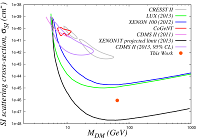
Figure 1: Various DM direct detection experimental bounds on the benchmark point of Table 1. See text for details.

The calculated branching ratio for the channel ${\rm LIP}~{}{\rm LIP}\to b\bar{b}$ is found to be 69.2%. The branching ratios for other annihilation channels in case of the present LIP dark matter are also computed and they are tabulated in Table 2. Since the DM mass is close to half of the SM Higgs ($\sim m_{h}/2$) like particle discovered by LHC, we will have resonance effect in obtaining the required cross-section ($2.37\times 10^{-26}$ cm³s^-1) with $b\bar{b}$ as dominant channel for the typical thermal production of DM. Also DM-nucleon scattering cross-section for the chosen benchmark point in this model is about $8.89\times 10^{-11}$ pb (averaged value per nucleon for interaction with Xe nucleus) which is just under the the present bounds for XENON 100 and LUX experiments. This is shown in Fig. 1. The future DM direct searches like XENON1T (Aprile, 2013) can easily probe this point as seen from Fig. 1.

The Fermi-LAT data for gamma-ray flux from the inner $5\arcdeg$ surrounding of the galactic centre have been studied in Ref. (Hooper, 2012). The known $\gamma$-ray sources in this region can be found in (extracted from) Fermi Second Source Catalog (2FGL) (Fermi-LAT Collaboration, 2012). Although Fermi Third Source Catalog (3FGL) has recently been made available (Fermi-LAT Collaboration, 2015), but no analysis of the background or analysis for $\gamma$-ray from other known processes at the region of interest has been reported yet. Also cosmic ray interaction with gas distributed in this galactic region produces neutral pions that subsequently decay to produce enormous amount of $\gamma$-ray. This is a viable mechanism for known disc template emission. Now, the spectral and morphological feature of the photon flux from inner $5\arcdeg$ subtending the GC after subtracting the contribution from both the known sources of Fermi Second Source Catalog and disc template emission shows a ‘bumpy’ nature in $\gamma$-ray energy ranging from $\sim$ 300 MeV to $\sim$ 10 GeV. The count drops significantly after 10 GeV of $\gamma$-ray energy.

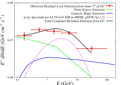
Figure 2: Residual GeV gamma-ray flux from the inner $5\arcdeg$ surrounding the galactic centre. See text for details.

We have computed the $\gamma$-ray spectrum from inner $5\arcdeg$ subtending the GC from DM annihilation within the present framework of inert Higgs doublet model for dark matter particle. The chosen benchmark points for the parameters of the model such as dark matter mass, coupling constants etc. are given in Table 1. The flux have been computed for the generalised NFW DM halo profile. Also included in the calculation are the contributions from both point source and galactic ridge emission. The total calculated flux is then compared with the observed residual photon flux and the results are shown in Fig. 2. In Fig. 2, the green-coloured and blue-coloured lines represent the fluxes for point source and galactic ridge emission respectively. The $\gamma$-ray spectrum for DM annihilation for the benchmark points mentioned above, are shown in purple line whereas the black line is for the total $\gamma$-ray flux obtained by summing over all the fluxes represented by green, blue and purple coloured lines in Fig. 2. For these calculations we have adopted the generalised NFW (gNFW) halo profile with $\gamma=1.26$. The total flux (black line) is then compared with the observed residual emission data. These observed data are denoted by red-coloured points in this figure. It is clear from Fig. 2 that our computation of total residual gamma emission (black line) agrees satisfactorily with the observational results.

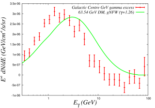
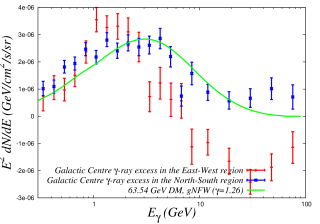
Figure 3: Left panel: Comparison of calculated $\gamma$-ray flux (green line; assuming DM annihilation) with the observed $\sim 1-3$ GeV gamma-ray excess from GC (red data points). Right panel: Same as the left panel but here the observed data are for galactic ‘North-South’ region ($|b|<|\ell|$; red data points) and for galactic ‘East-West’ region ($|b|>|\ell|$; blue data points). See text for details.

In a recent analysis of $\gamma$-ray flux from GC region where the analysis is only for the GC gamma ray (subtracting all possible contributions from other known astrophysical sources), (Daylan et al., 2014) an excess of gamma ray in the gamma energy region of $\sim 1-3$ GeV has been reported. This excess is shown in the left panel of Fig. 3 with the red-coloured points. It is suggested in the same analysis that in order to explain this anomalous gamma ray excess from dark matter annihilation scenario, the DM mass should be in the range of 31-40 GeV which is to annihilate purely into $b\bar{b}$ pair. We calculated these gamma ray fluxes in our framework of inert Higgs doublet dark matter for the dark matter mass of $\sim$ 63.5 GeV (adopted from Table 1 (benchmark point)) and compared our results with the analysed data points mentioned above (red coloured points shown in the left panel of Fig. 3). In the left panel of Fig. 3, the green coloured line represents the present calculation. These calculations are performed considering gNFW halo profile with the halo parameter $\gamma=1.26$. It is to be noted from the left panel of Fig. 3 that although the morphological feature of the spectrum from our calculation (green line) is similar in nature to that obtained from the analysis of Fermi-LAT observational data (red-coloured points) from GC, the position of the maxima of excess gamma ray in our calculation is shifted to somewhat higher energy at $\sim 3.1$ GeV instead of being within the expected energy range of $\sim 1-3$ GeV as obtained from the Fermi-LAT data. However the calculated position of the peak (green line) is at $\sim 2.84\times 10^{-6}$ GeV/cm²/s/sr which is in the same ballpark of the observed peak (red points).

More detailed analysis of the observed $\gamma$-ray excess reveals (Daylan et al., 2014) a further anomaly between the gamma ray spectra for the gamma rays from galactic East-West region and from galactic North-South region. The North-South region is designated as $|b|<|\ell|$, where $b$ and $\ell$ are the galactic latitude and longitude respectively and for the East-West region, $|b|>|\ell|$. The two spectra are shown in the right panel of Fig. 3. The red coloured points are for gamma spectrum from galactic East-West region while the blue coloured points represent the spectrum from North-South region. As can be seen from the right panel of Fig. 3, the gamma flux from the present calculation (shown by green line in the right panel of Fig. 3) agrees more satisfactorily with the “North-South” gamma emission spectrum than the “East-West” spectrum.

The systematic uncertainty for the estimation of background model provided by the Fermi-LAT is very large compared to the statistical uncertainty. Attempts (Calore et al., 2014b; Murgia, 2014) are made to quantify such systematics for galactic central region. We confront the flux obtained for our IHDM benchmark scenario (Table 1) using these two complementary approaches. We adopt the proposed method of Ref. (Agrawal et al., 2014a) for the uncertainty estimation of $J$-factor. This involves estimation of halo profile uncertainty and the uncertainty in local DM density. The density profile index $\gamma$, is estimated to be $\gamma=1.2\pm 0.1$ from different galactic diffuse emission models and $\rho_{\odot}$ is estimated to be $\rho_{\odot}=0.4\pm 0.2$ GeV/cm³ for different normalisation of halo.Defining the $J$-factor as

$$\bar{J} =\frac{1}{\Delta\Omega}\int_{\Delta\Omega}J(\psi)d\Omega\equiv\mathbb{J}\times\bar{J}_{\rm canonical}\,,$$ (3.5)

where $\bar{J}_{\rm canonical}$ is the central value of $\bar{J}$ and the factor $\mathbb{J}$ signifies the deviation from the canonical halo profile due to the uncertainties of the profile. In the above $\Delta\Omega$ is the region of interest (ROI) for a given analysis. The astrophysical factor $J(\psi)$ is same as that in Eq. 3.2.

In Ref. (Calore et al., 2014b) a thoroughly analysis of Fermi-LAT data in the inner galaxy region over the photon energy ranging from 300 MeV – 500 GeV has been made where the chosen region of interest (ROI) is extended to a $20^{\circ}\times 20^{\circ}$ ($-20^{\circ}<\ell<20^{\circ}$, $-20^{\circ}<b<20^{\circ}$) square region surrounding the galactic centre. The inner galactic latitude of $2^{\circ}$ ($|b|<2^{\circ}$) has been masked out. For the canonical halo profile with $r_{\odot}=8.5$ kpc, $\rho_{\odot}=0.4$ GeV/cm³, $r_{c}=20$ kpc and $\gamma=1.20$. The numerical value of $\bar{J}_{\rm canonical}$ is found out to be $2.0\times 10^{23}$ GeV² cm^-5 for the canonical halo. The uncertainty ($\mathbb{J}\in[0.19,3]$) in the $\bar{J}$ factor is found out to be in their analysis.

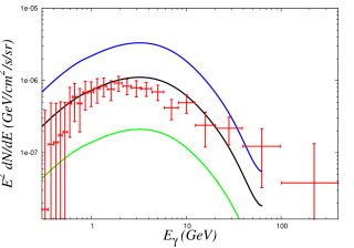
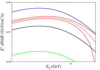
Figure 4: Left panel: Comparison of calculated $\gamma$-ray flux (red points) with the observed residual $\gamma$-ray spectrum for the region in galactic coordinate $|\ell|<20^{\circ}$, $2^{\circ}<|b|<20^{\circ}$. The black line is for canonical $J$-factor while green and blue lines are calculated with minimum and maximum deviations of $J$-factor from its canonical value. Right panel: Comparison of the calculated results in the left panel with observed $\gamma$-ray spectra (red points) obtained by studying $15^{\circ}\times 15^{\circ}$ region around GC. See text for details.

Plugging in all of the canonical parameters for the dark matter halo model, we compute the canonical $\gamma$-ray flux obtained from annihilation channels of $\sim$ 63.5 GeV LIP DM (adopted from Table 2 (benchmark point)). The resulting plot is shown in the left panel of Fig. 4 by black coloured line. The black line is obtained considering only the canonical value $\mathbb{J}\in[0.19,3]$ of the $J$-factor. The red coloured points denote the residual spectrum of $\gamma$-ray excess in the galactic centre with highly correlated errors obtained from Ref. (Calore et al., 2014b). We repeat the calculations by also taking the uncertainties $\mathbb{J}\in[0.19,3]$ in the $\bar{J}$ factor. The blue and the green coloured lines in the left panel of Fig. 4 denote the galactic $\gamma$-ray flux from $\sim$ 63.5 GeV DM annihilation for the maximum value of the uncertainty $\mathbb{J}_{\rm max}\sim 3.0$ and the minimum value of the uncertainty $\mathbb{J}_{\rm min}\sim 0.19$ respectively. From the left panel of Fig. 4 one sees that the uncertainty factor $\mathbb{J}$ needs to be smaller than unity to have a better fit to the data.

On the other hand, recently the Fermi collaboration (Murgia, 2014) has also studied the region surrounding the galactic centre using different background models of galactic diffuse emission. The fit to the galactic centre $\gamma$-ray data is observed to improve very significantly when an additional contribution similar to that from dark matter annihilation is added. The Fermi collaboration has chosen a different region ($15^{\circ}\times 15^{\circ}$) surrounding the galactic centre smaller than that chosen by Ref. (Calore et al., 2014b). However for their analysis, unlike in Ref. (Calore et al., 2014b), in this case, the galactic centre is not masked out. Based on their preliminary analysis the Fermi collaboration has reported four best fit $\gamma$-ray spectra for the four distinct choices of background models for galactic diffuse emission. The nature of these four best fit $\gamma$-ray spectra differ notably after a few GeV photon energy. The obtained $\gamma$-ray spectra is found to yield much more conservative measurement of the systematic uncertainty. Although the Fermi has analysed the data using NFW halo profiles with slope values of 1.0 and 1.2, Ref. (Agrawal et al., 2014a) has chosen a more conservative approach on $\gamma$ factor and set it to $1.2\pm 0.1$. Also the value of $\rho_{\odot}$ is chosen to be $0.4\pm 0.2$ GeV/cm³. Keeping the parameters of the $J$-factor fixed, one would obtain in this case, $\bar{J}_{\rm canonical}=1.58\times 10^{24}$ GeV² cm^-5. The uncertainty in the $\bar{J}$ factor as obtained from such parametrisation is $\mathbb{J}\in[0.14,4.0]$ for the Fermi analysis.

We make an estimation of the galactic $\gamma$-ray excess from the annihilation of dark matter as chosen in this work (benchmark point in Table 1) and confront the results with the $\gamma$-ray spectra obtained by Fermi collaboration. We make the comparison of the calculated spectrum with that reported by Fermi after preliminary analysis and show it in the right panel of Fig. 4. The black line in the right panel of Fig. 4 denotes the photon flux obtained using the canonical parametrisation of the halo profile (with $\mathbb{J}=1$). The blue and the green coloured lines in the right panel of Fig. 4 represent the galactic $\gamma$-ray flux calculated for the maximum uncertainty $\mathbb{J}_{\rm max}\sim 4.0$ and the minimum uncertainty $\mathbb{J}_{\rm min}\sim 0.14$ respectively. Also shown in the right panel of Fig. 4 the Fermi analysis results with its upper and lower bounds.  From the right panel of Fig. 4 it appears that unlike the previous analysis (with $-20^{\circ}<\ell,b<20^{\circ}$) the uncertainty factor $\mathbb{J}$ should be more than unity in order to provide a better fit to the data for the considered IHDM benchmark point.

4 Confronting Gamma-ray flux from Dwarf Spheroidal Galaxies in this framework

One of the most promising targets for the search of dark matter via indirect detection ($\gamma$-ray) is the dwarf spheroidal galaxies (dSphs) of the Milky Way. The dSphs are considered to be promising for the study of DM phenomenology because of their proximity, low astrophysical background and huge amount of DM content.

The satellite-bourne gamma-ray experiment, Fermi-LAT, search for the $\gamma$-ray sky in the energy range spanning from $\sim$ 500 MeV – 500 GeV (Atwood et al., 2009). In a more recent study by Ackermann et al.  (Ackermann et al., 2014), 4-year gamma ray data of Fermi-LAT on dSphs (04-08-2008 to 04-08-2012) with energy ranging from 500 MeV to 500 GeV have been chosen for studying 25 independent Milky Way dSphs galaxies. The chosen dSphs galaxies are Bootes I, Bootes II, Bootes III, Canes Venatici I, Canes Venatici II, Canis Major, Carina, Coma Berenices, Draco, Fornax, Hercules, Leo I, Leo II, Leo IV, Leo V, Pisces II, Sagittarius, Sculptor, Segue 1, Segue 2, Sextans, Ursa Major I, Ursa Major II, Ursa Minor and Willman 1. The galactic coordinates as well as the radial distances from the galactic centre of these dwarf galaxies are tabulated in Table 3. From the analysis of their data, they set robust upper limits on DM annihilation cross-section for different DM masses. In giving this limits, they consider the DM pair annihilate predominantly to $b\bar{b}$ as also $\tau\bar{\tau}$ and other channels.

It is possible to assess the total DM content of dSphs galaxies from the dynamical modeling of the stellar density of the dwarf galaxies and the velocity dispersion profiles (Battaglia et al., 2013; Walker et al., 2009b; Wolf et al., 2010). The dynamical masses of these dwarf galaxies are measured only from stellar velocity dispersion and half-light radius. The calculated total mass within the half-light radius for a dSphs galaxy is used to obtain the integrated $J$-factor of that dSphs galaxy. Both the total mass within the half-light radius and the $J$-factor are found to be almost independent on the choice of DM halo profiles (Martinez et al., 2009; Strigari, 2013; Martinez, 2013). Out of the 25 independent dSphs mentioned earlier, $J$-factors of only 18 dSphs are determined using stellar kinematics data (Martinez, 2013) while other seven lack proper statistical significances. Using these uncertainties of $J$-factors, the upper bounds on DM annihilation cross-section for various DM masses have been derived with 95% CL.

We calculate the $\gamma$-ray flux for all the dwarf galaxies. The $\gamma$-ray spectrum, $\frac{dN}{dE}$ can be obtained for a given DM mass. The different particle processes for the calculation of $\frac{dN}{dE}$ are tabulated in Table 2. We compute $\frac{dN}{dE}$ for our benchmark scenario and using the integrated $J$-factor for a particular dSph, the maximum value of the velocity-averaged annihilation cross-section ($\langle\sigma v\rangle_{\rm max}$) is estimated from the upper bound of the flux (LHS of Eq. 3.1) of that dSph. In this way the upper bounds of annihilation cross-section are computed for all the 18 dSphs considered and they are tabulated in Table 3.

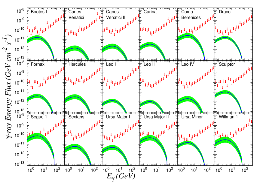
Figure 5: Comparison of computed $\gamma$-ray flux with the bin-by-bin integrated $\gamma$-ray energy-flux upper limits for each dSph. The downward red-coloured arrows represent bin-by-bin upper limits on the $\gamma$-ray energy-flux at 95% CL. The blue lines denote the $\gamma$-ray fluxes calculated using the central values of integrated $J$-factor whereas the green band is for the uncertainties in the measurement of integrated $J$-factors for 18 Milky Way dSphs. See text for details.

We now compute the $\gamma$-ray flux for all the 18 dSphs considered using Eq. 3.1. The maximum, minimum and central values of integrated $J$-factor for each dwarf galaxy which are measured from stellar kinematics data are tabulated in Table 3 (Ackermann et al., 2014). The integration to find $J$-factor involves integration over a solid angle $\Delta\Omega$ of $\sim 2.4\times 10^{-4}$ sr (the field of view of Fermi-LAT is within the angular radius of $0.5\arcdeg$). The results are shown in the plots given in Fig. 5.We also show in Fig. 5 the experimentally obtained bin-by-bin upper limits of the gamma ray energy flux at 95% CL from each dwarf galaxy by downward red-coloured arrows. The flux of a dSph are compared with the upper bound of the flux in each energy bin. The spread (band) of this flux shown by green indicate the upper and lower limits of the flux when calculated with the upper and lower limits of integrated $J$-factors. The photon flux calculated using the central value of $J$-factors are shown by blue lines in these figures.

5 Confronting Extragalactic gamma ray background in this framework

The $\gamma$-rays can also be emitted from DM annihilation in extragalactic sources and such $\gamma$-rays can be probed for extragalactic DM and their origins (Ullio et al., 2002; Bergstrom et al., 2001; Gao et al., 1991; Stecker, 1978; Taylor & Silk, 2003; Ng et al., 2014; Ando, 2005; Oda et al., 2005; Pieri et al., 2008). Such gamma rays from extragalactic sources of DM can remain hidden in the huge background of the observationally measured gamma flux by satellite-borne experiments such as SAS-2 satellite (Fichtel et al., 1978), EGRET (Sreekumar et al., 1998), Fermi-LAT (Abdo et al., 2010b; Ackermann et al., 2015b). In order to extract information regarding the extragalactic signature of gamma rays from the background one should be able to understand and subtract the galactic astrophysical components, other sources that may contribute to the background and the backgrounds that the detector may give rise to, in the process of detection. After this process of subtraction the residual gamma-ray signal thus obtained is found to be diffuse and isotropic in nature and is known as diffuse isotropic gamma-ray background (DIGRB). Recently in the light of 50-month Fermi-LAT data an updated tight constraint on DM annihilation is given with the modelling of integrated emission of blazars with such diffuse background absorption (Ajello et al., 2015). This may also be noted that the DIGRB thus obtained embeds in it the irreducible contributions from galactic origin as well. In this section we estimate such diffuse isotropic gamma ray background or DIGRB for the case of dark matter annihilating into gamma rays in the framework of the chosen IHDM dark matter candidate. We then compare our theoretical calculations with EGRET and Fermi-LAT results for extragalactic DIGRB.

5.1 Formalism

The number of photons which are isotropically emitted from the volume element $dV$ in time interval $dt$, in energy range $dE$ and are collected by detector with effective area $dA$ during time interval $dt_{0}$ with redshifted energy range $dE_{0}$ can be given by (Ullio et al., 2002),

$$dN_{\gamma}=e^{-\tau(z,E_{0})}\left[(1+z)^{3}\,\int dM\;\frac{dn}{dM}(M,z)\,\frac{d{\cal N}_{\gamma}}{dE}\left(E,M,z\right)\right]\;\frac{dV\,dA}{4\pi[R_{0}S_{k}(r)]^{2}}\,dE_{0}\,dt_{0}\;.$$ (5.1)

In the above, the volume element $dV$ at a redshift $z$ is given as

$$dV=\frac{[R_{0}S_{k}(r)]^{2}\,R_{0}}{(1+z)^{3}}drd\Omega_{\rm detector}\;,$$ (5.2)

where $d\Omega_{\rm detector}=\sin\theta d\theta d\phi$ denotes the angular acceptance of the detector. In Eq. 5.1 and Eq. 5.2, $S_{k}(r)$ is given by the Robertson Walker metric for homogeneous and isotropic universe

$$ds^{2}=c^{2}dt^{2}-R^{2}(t)\left[dr^{2}+S_{k}^{2}(r)(d\theta^{2}+\sin^{2}\theta d\phi^{2})\right]\;,$$ (5.3)

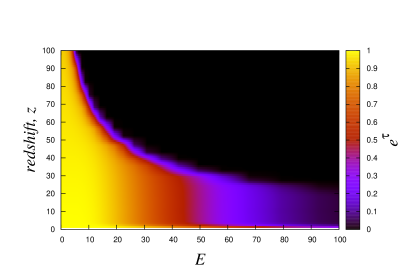
Figure 6: The variation of optical depth (transparency coefficient) $e^{\tau}$ with the energy at detection ($E$) and the redshift ($z$) of photon emission for minimum UV background model. The black zone in this figure represents total opaque region while the yellow zone is for total transparent one. See text for details.

where $S_{k}(r)$ signifies the spatial curvature of the universe. In Eq. 5.1, $\frac{d{\cal N}_{\gamma}}{dE}\left(E,M,z\right)$ is the differential photon energy spectrum for a generic halo with mass $M$ at some redshift $z$. The term $\frac{dn}{dM}(M,z)$ is the halo mass function and is defined as number density of bound objects with mass $M$ at redshift $z$. The term $e^{-\tau(z,E_{0})}$ represents the attenuation of extragalactic $\gamma$-rays which may come from the absorption of these high energy $\gamma$-rays on the extragalactic background light (EBL) and $\tau(z,E_{0})$ is the optical depth which is function of $z$ and $E_{0}$. The energy and redshift dependence of this attenuation factor is shown in Fig. 6. Detailed studies regarding this attenuation are given in Ref. (Cirelli et al., 2011). For ultraviolet background we have adopted the minimal model (Dominguez et al., 2011; Franceschini et al., 2008) obtained after a recent study on blazars. Note that $dt_{0}dE_{0}$ in Eq. 5.1 is given by $dtdE=\frac{dt_{0}}{(1+z)}.(1+z)dE_{0}$, where $t_{0}$ and $E_{0}$ are the time and energy respectively corresponding to the redshift $z=0$. Summing over all the above contributions, the diffuse extragalactic $\gamma$-ray flux due to DM annihilation, can be written as,

$$\frac{d\phi_{\gamma}}{dE_{0}}\equiv\frac{dN_{\gamma}}{dA\,d\Omega\,dt_{0}\,dE_{0}} = \frac{1}{4\pi}\int dr\,R_{0}e^{-\tau(z,E_{0})}\int dM\;\frac{dn}{dM}(M,z)\,\frac{d{\cal N}_{\gamma}}{dE}\left(E_{0}\,(1+z),M,z\right)$$ (5.4)

$$= \frac{c}{4\pi}\int dz\frac{e^{-\tau(z,E_{0})}}{H_{0}\,h(z)}\int dM\;\frac{dn}{dM}(M,z)\,\frac{d{\cal N}_{\gamma}}{dE}\left(E_{0}\,(1+z),M,z\right)\;,$$

where $c$ is the speed of light in vacuum, $H_{0}$ is the Hubble constant at the present epoch and $h(z)$ is written as (for spatially flat universe ($\Omega_{k}=0$))

$$h(z)=\sqrt{\Omega_{M}(1+z)^{3}+\Omega_{\Lambda}}.$$ (5.5)

where $\Omega_{M}$ and $\Omega_{\Lambda}$ are respectively the matter and dark energy densities normalised to the critical density of the universe. The cosmological dark matter halo function $\frac{dn}{dM}(M,z)$ in Eq. 5.4 can be written in the form (Press & Schechter, 1974),

$$\frac{dn}{dM}=\frac{{\rho}_{0,m}}{M^{2}}\nu f(\nu)\frac{d\,\log\nu}{d\,\log M}\;,$$ (5.6)

where ${\rho}_{0,m}$ is the comoving background matter density. In the above, the parameter $\nu=\delta_{\rm sc}/\sigma(M)$, defined as the ratio between the critical overdensity for spherical collapse $\delta_{\rm sc}$ ($\simeq 1.686$) and $\sigma(M)$ denotes the variance or the root mean square density fluctuations of the linear density field in sphere that contains the mean mass $M$. The term $\sigma^{2}(M)$ can be written in terms of the linear power spectrum $P(k)$ of the fluctuations (Sheth & Tormen, 1999) as,

$$\sigma^{2}(M)\equiv\int d^{3}k\;\tilde{W}^{2}(kR)\,P(k)\,\,\,,$$ (5.7)

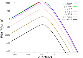
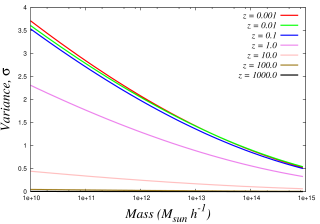
Figure 7: The variation of the linear power spectrum $P(k)$ of matter density perturbations with the wavenumber $k$ of the fluctuations for different redshifts is shown in the left panel. In the right panel the variance $\sigma$ of the density perturbations is shown as a function of halo mass for different redshifts. In both plots the values of redshift $z=10^{-3},10^{-2},10^{-1},10^{0},10^{1},10^{2}\ \mathrm{and}\ 10^{3}$. See text for details.

where $\tilde{W}(kR)$ is the Fourier transform of the top hat window function and $R$ is the comoving length scale. For collapsed halos, the mass is found to be in the form $M\simeq(4/3)\pi R^{3}\rho_{c}(z_{c})$ with $z_{c}$ being the redshift where collapsing of halos occurs. The power spectrum $P(k)$ can be parametrised as $P(k)\propto k^{n}T^{2}(k)$ where $n$ is the spectral index and $T$ is the transfer function that incorporates the effect of scale dependency of the primordial power spectrum generated during inflation. This transfer function depends on the nature of DM and baryon density in the universe. Thus the transfer function can be calculated from the cosmic microwave background data. The variation of the power spectrum $P(k)$ with wavenumber $k$ for different redshifts is shown in the left panel of Fig. 7. The right panel of Fig. 7 corresponds to the plot showing the variation of variance $\sigma$ with halo mass $M$ for different values of redshift. The function $f(\nu)$ in Eq. 5.6, known as the multiplicity function, can be modelled in the ellipsoidal collapse model (Sheth & Tormen, 1999) by,

$$\nu f(\nu)=2A\left(1+\frac{1}{\nu^{\prime 2p}}\right)\left(\frac{\nu^{\prime 2}}{2\pi}\right)^{1/2}\exp\left(-\frac{\nu^{\prime 2}}{2}\right)\,\,\,,$$ (5.8)

where $\nu^{\prime}=\sqrt{a}\nu,a=0.707,p=0.3$ are obtained by fitting Eq. 5.6 to $N$-body simulation of Virgo consortium (Jenkins et al., 1998). The value of $A$ is obtained to be $0.3222$ For the choice of parameter values, $a=1,p=0$ and $A=0.5$, Eq. 5.6 reduces to the original Press-Schechter theory (Press & Schechter, 1974). It is found in $N$-body simulations that the estimations of higher and lower mass halos differ from that predicted by Press-Schechter model. This problem can be handled in Sheth-Torman model by considering ellipsoidal collapse model instead of spherical one.

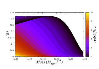
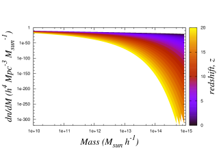
Figure 8: The fraction of mass collapsed, $f(\sigma)$ in Sheth-Torman model for different redshifts $z$ and the halo masses $M$ is shown in left panel. The variation of Sheth-Torman halo mass function ${dn\over dM}$ with the redshift $z$ and the halo mass $M$ is shown in right panel. See text for details.

In the left panel of Fig. 8 the variations of the fraction of mass collapsed or $f(\sigma)$ in the ellipsoidal collapse model with redshifts $z$ and the halo mass $M$ are shown. Note that $f(\sigma)$ as shown in the left panel of Fig. 8 can be obtained by simple transformation of $f(\nu)$ by plugging in $\nu=\delta_{\rm sc}/\sigma(M)$ and is given by $f(\sigma)=A\sqrt{\frac{2a}{\pi}}\left[1+\left(\frac{\sigma^{2}}{a\delta_{\rm sc}^{2}}\right)^{p}\right]\frac{\delta_{\rm sc}}{\sigma}\exp\left[-\frac{a\delta_{\rm sc}^{2}}{2\sigma^{2}}\right]$. In the right panel of Fig. 8 we have shown the variations of the considered halo mass function $dn/dM$ of Sheth-Torman model (Sheth & Tormen, 1999) with redshift $z$ as well as with the halo mass $M$. All the numerical calculations related to Fig. 8 have been performed using HMFcalc (Murray et al., 2013) code.

For the halo profile we have chosen NFW halo profile (Navarro et al., 1996, 1997) given by,

$$\rho(r)=\rho_{s}\,g(r/r_{s})=\rho_{s}{1\over{r\over r_{s}}\left(1+{r\over r_{s}}\right)^{2}}\;,$$ (5.9)

Any DM halo of mass $M_{h}$ enclosed at a radius $r_{h}$ is,

$$M_{h}=4\pi\rho_{s}r_{h}^{3}f(r_{s}/r_{h})\,\,\,,$$ (5.10)

where $f(x)=x^{3}[\ln(1+x^{-1})-(1+x)^{-1}]$.

Also a halo of mass $M$ at some redshift $z$ can be written in terms of mean background $\bar{\rho}(z)$ as,

$$M\equiv{4\pi\over 3}\Delta_{vir}\bar{\rho}(z)\,R_{vir}^{3}\,\,\,,$$ (5.11)

where $R_{vir}$ is the virial radius defined as the radius within which the total halo mass $M$ is contained with mean halo density $\Delta_{vir}\bar{\rho}(z)$. The term $\Delta_{vir}$ is the virial overdensity with respect to the mean matter density which may depend on the cosmological parameters but independent of halo mass $M_{h}$. For the flat cosmology, $\Delta_{vir}(z)$ can be cast into the following form (Bryan & Norman, 1998),

$$\Delta_{vir}\simeq(18\pi^{2}+82d-39d^{2})\,\,\,,$$ (5.12)

with $d\equiv d(z)={\Omega_{m}(1+z)^{3}\over(\Omega_{m}(1+z)^{3}+\Omega_{\Lambda})}-1$. We choose the value of $\Delta_{vir}(z)$.

The $\gamma$-ray energy spectrum $\frac{d{\cal N}_{\gamma}}{dE}\left(E_{0}\,(1+z),M,z\right)$ (Eq. 5.4) for the gamma-ray emitted inside a halo of mass $M$ at redshift $z$ is written to the form,

$$\frac{d{\cal N}_{\gamma}}{dE}(E,M,z)=\frac{\langle\sigma v\rangle}{2}\frac{dN_{\gamma}(E)}{dE}\int dc^{\,\prime}_{vir}\;{\cal{P}}(c^{\,\prime}_{vir})\left(\frac{\rho^{\prime}}{M_{\chi}}\right)^{2}\int d^{3}r\;g^{2}(r/a)\;,$$ (5.13)

where $\langle\sigma v\rangle$ is the thermally averaged value of annihilation cross-section times the relative velocity, $\frac{dN_{\gamma}(E)}{dE}$ is the differential $\gamma$-ray energy spectrum produced per unit annihilation of dark matter and $M_{\chi}$ is the mass of dark matter. The log-normal distribution ${\cal{P}}(c_{vir})$ of the concentration parameter $c_{vir}$ around the mean value is chosen within $1\sigma$ deviation (Sheth & Tormen, 2004), for halos with mass $M$. Finally one can write,

$$\frac{d{\cal N}_{\gamma}}{dE}(E,M,z)=\frac{\sigma v}{2}\frac{dN_{\gamma}(E)}{dE}\frac{M}{M_{\chi}^{2}}\,\frac{\Delta_{vir}\bar{\rho}(z)}{3}\,\int dc^{\,\prime}_{vir}\;{\cal{P}}(c^{\,\prime}_{vir})\frac{(c^{\,\prime}_{vir}\,r_{-2})^{3}}{\left[I_{1}(c^{\,\prime}_{vir}\,r_{-2})\right]^{2}}\,I_{2}(x_{min},c^{\,\prime}_{vir}\,r_{-2})\;.$$ (5.14)

In the above $r_{-2}$ is the ratio between $r_{s}^{(-2)}$ and $r_{s}$ where $r_{s}^{(-2)}$ is the radius at which the effective logarithmic slope $-2$ that follows from the relation, $d/dr\left.\left(r^{2}g(r)\right)\right|_{r=r_{s}^{(-2)}}=0$. For NFW profile, $r_{s}^{(-2)}=r_{s}$. Hence $c_{vir}r_{-2}=R_{vir}/r$ and the form of integration $I_{n}(x_{min},x_{max})$ in Eq. 5.14 can be cast into the form,

$$I_{n}(x_{min},x_{max})=\int_{x_{min}}^{x_{max}}dx\,x^{2}g^{n}(x)\;.$$ (5.15)

Plugging the above equation in Eq. 5.4, the analytic form of extragalactic gamma-ray flux from DM annihilation can be obtained as (Ullio et al., 2002)

$$\frac{d\phi_{\gamma}}{dE_{0}}=\frac{\sigma v}{8\pi}\frac{c}{H_{0}}\frac{{\rho}_{0}^{2}}{M_{\chi}^{2}}\int dz\;(1+z)^{3}\frac{\Delta^{2}(z)}{h(z)}\frac{dN_{\gamma}(E_{0}\,(1+z))}{dE}e^{-\tau(z,E_{0})}\;,$$ (5.16)

where the expression for $\Delta^{2}(z)$ can be given by,

$$\Delta^{2}(z)\equiv\int dM\frac{\nu(z,M)f\left(\nu(z,M)\right)}{\sigma(M)}\left|\frac{d\sigma}{dM}\right|\Delta_{M}^{2}(z,M)\;$$ (5.17)

with

$$\Delta_{M}^{2}(z,M)\equiv\frac{\Delta_{vir}(z)}{3}\,\int dc^{\,\prime}_{vir}\;{\cal{P}}(c^{\,\prime}_{vir})\frac{I_{2}(x_{min},c^{\,\prime}_{vir}(z,M)\,r_{-2})}{\left[I_{1}(x_{min},c^{\,\prime}_{vir}(z,M)\,r_{-2})\right]^{2}}(c^{\,\prime}_{vir}(z,M)\,r_{-2})^{3}\;.$$ (5.18)

In all of the above the concentration parameter, $c_{vir}$ is defined as

$$c_{vir}=\frac{R_{vir}}{r_{s}^{(-2)}}\,\,\,,$$ (5.19)

We have chosen two forms of concentration parameter $c_{vir}$ following Macciò et al. (Maccio’ et al., 2008) and power law model (Neto et al., 2007; Maccio’ et al., 2008). For the first choice (Macciò et al.), $c_{vir}(M,z)=k_{200}\left(\mathcal{H}(z_{f}(M))/\mathcal{H}(z)\right)^{2/3}$, where $k_{200}\simeq 3.9$, $\mathcal{H}(z)=H(z)/H_{0}$ and $z_{c}(M)$ is the effective redshift during the formation of a halo with mass $M$. In the power law model (second choice) however the expression of $c_{vir}(M,z)$ is adopted as $c_{vir}(M,z)=6.5\,\mathcal{H}(z)^{-2/3}$ $(M/M_{*})^{-0.1}$, $M_{*}=3.37\,10^{12}h^{-1}M_{\odot}$. This choice of $c_{vir}(M,z)$ provides a reasonable fit within the resolved mass range in the simulations.

The dark matter substructures are present within halo and form bound objects. The mass of the smallest possible such bound object (subhalo) is denoted as $M_{\rm min}$. The value of this minimum subhalo mass, $M_{\rm min}$ is determined from the temperature at which the DM particles just start decoupling kinematically from the cosmic background.

In this work we perform our analysis for two typical values of $M_{\rm min}$; $M_{\rm min}=10^{-6}M_{\odot}$ and $10^{-9}\,M_{\odot}$ (Martinez et al., 2009; Bringmann, 2009). The boost factor for $\gamma$-ray flux due to these subhalos depends inversely on $M_{\rm min}$.

5.2 Non-DM Contributions in DIGRB

The extragalactic gamma-ray spectrum in the energy range between $\sim$ few hundred MeV and $\sim$ few hundred GeV as observed by the Fermi-LAT telescope is found to follow almost a power law spectrum (${dN_{\gamma}\over dE}\propto E^{-2.41}$). There are contributions from astrophysical sources other than that from possible dark matter annihilation (Tavakoli et al., 2014). The possible sources that contribute to the diffuse $\gamma$-ray background other than the DM include BL Lacertea objects (BL Lacs), flat spectrum radio quasars (FSRQs), millisecond pulsars (MSPs), star forming galaxy (SFG), Fanarof-Riley (FR) radio galaxies of type I (FRI) and type II (FRII), ultra high energy cosmic rays (UHECRs), gamma ray bursts (GRBs), star burst galaxy (SBG), Ultra High Energy protons in the inter-cluster material (UHEp ICM) and gravitationally induced shock waves (IGS) etc. The spectral features of photon spectra originated from the non-DM objects (Tavakoli et al., 2014) considered in this work are concisely summarised in Table 4.

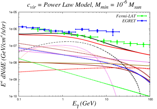
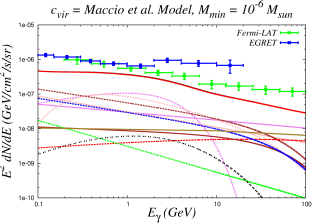
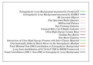
Figure 10: The observed extragalactic $\gamma$-ray fluxes by EGRET and Fermi-LAT are compared with the sum total value of the $\gamma$-ray fluxes obtained from the present calculation. The calculated value of extragalactic $\gamma$-ray flux is obtained by summing over the $\gamma$-ray flux calculated from DM annihilation for IHDM LIP DM (considered in this work) and other possible $\gamma$-rays (extragalactic $\gamma$-ray sources of non-DM origin) from extragalactic sources. See text for details.

We add up the contributions to EGB both from the annihilating DM in IHDM framework ($\sim$ 63.5 GeV DM considered in this work) and the other possible non-DM astrophysical sources. The comparison of the sum total value of the $\gamma$-ray flux with the observed EGB by EGRET and Fermi-LAT is shown in Fig. 10. Needless to mention here that the four plots in Fig. 10 are for different parametrisations of concentration parameter $c_{vir}$ and subhalo mass $M_{\rm min}$. As mentioned earlier we have considered BL Lacs, FSRQs, MSPs, SFGs, FR (type I and II), UHECR, GRBs, SBGs, UHEp interacting with ICM and IGS as contributors to EGB other than DM and their contributions to EGB are shown with different lines in Fig. 10. The computed total photon spectra in the plots of Fig. 10 are shown by black solid lines while the red solid line is for the minimal non-DM contribution to EGB. The black lines are found to be on top of the red lines for Macciò et al. models.

We also mention that the extragalactic $\gamma$-ray signal is analysed within the dark matter annihilation scenario in Ref. (Cholis et al., 2014). In their analysis they have constructed a model for the non-DM astrophysical contributions to the extragalactic $\gamma$-ray background and they have also adopted a substructure model based on numerical simulations. The authors in Ref. (Cholis et al., 2014) have considered subhalo boost factor $b_{sh}$ in their analyses to be the following form (Ando & Komatsu, 2013)

$$b_{sh}(M)\approx 110\times(M_{200}/10^{12}M_{sun})^{0.39}$$ (5.20)

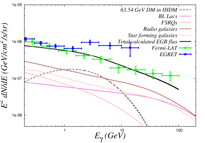
Figure 11: Comparison of the observed $\gamma$-ray fluxes by EGRET and Fermi LAT theoretical results for $\gamma$-ray spectra for $\sim$ 63.5 GeV DM in IHDM considering the modelling of extragalactic and astrophysical parameters as done in Ref. Cholis et al. (2014). See text for details

where $M_{200}$ denotes the mass enclosed within a radial region where the avaraged density is 200 times more than the critical density of the universe. We have performed the calculation of extragalactic photon flux for DM for the best-fit model parameter in IHDM based on their extragalactic modelling. The result is shown in Fig. 11. In Fig. 11 we have only considered the contributions to EGB only from radio galaxies, BL lacs, FSRQs and SFGs other than that from DM annihilation. The sum total contributions to EGB is found to fit reasonably well with Fermi-LAT data.

5.3 Galactic (sub)halo contribution to DIGRB

There could be a significant contribution to DIGRB which is of galactic origin along the line of sight due to the passing of the signal from extragalactic sources through the Milky Way galactic halos and subhalos. From numerical simulation the main DM halo is found to host a large amount of substructures in form of subhalos (Springel et al., 2008b; Diemand et al., 2007).

The signal from the DM annihilation at the galactic substructures could potentially give rise to an almost isotropic signal since this generated $\gamma$-ray flux is proportional to the less centrally concentrated number density distribution of subhalos (Springel et al., 2008a). The averaged photon intensity from DM annihilation in such smooth halo of the Milky Way can be written as,

$$\frac{dI_{\rm sm}(E_{\gamma})}{dE_{\gamma}}=\frac{\langle\sigma v\rangle}{2m_{\rm DM}^{2}}\frac{dN_{\gamma}}{dE_{\gamma}}\frac{1}{\Omega_{e}}\int_{V_{*}}dV~{}\frac{\rho_{\rm MW}^{2}(s,b,\ell)}{4\pi s^{2}},$$ (5.21)

where $s$ and $\Omega_{e}$ are the distance from the galactic centre and the observed solid angle. In the above $b$ and $\ell$ are galactic coordinates (latitude and longitude respectively) chosen to be $30^{\circ}\leq|b|\leq 90^{\circ}$, $0\leq\ell<2\pi$ (Cholis et al., 2014). $r_{s,{\rm MW}}=21.5$ kpc, $r_{\rm vir,MW}=258$ kpc, $\rho_{s,{\rm MW}}=4.9\times 10^{6}\,M_{\odot}$ kpc^-3, $M_{\rm vir,MW}=1.0\times 10^{12}\,M_{\odot}$ (Klypin et al., 2002) are chosen for our calculation. 

The photon flux produced in the smooth halo component are much subdominant than that yielded in the subhalos and hence they contribute negligibly to extragalactic $\gamma$-ray background. In $\Lambda$CDM cosmology, the formation of the structures is assumed to be hierarchical. The smaller DM halos are formed first and the larger ones later. In the period of structure formation the smaller halos are tidally disrupted after being captured by the larger host halos of galaxies and clusters and hence the outer low density layers are stripped in this process. Thus the central dense cores only survive and behave as subhalos of the host halos. These substructures of DM halo enrich DM phenomenology by giving rise to substantially enhancement of the DM annihilation rates within a halo. The contribution to differential gamma-ray flux from subhalo can be obtained from the differential luminosity profile of each subhalo which is given by,

$$\frac{dL_{\gamma}}{dE_{\gamma}}=\frac{\langle\sigma v\rangle}{2m_{\rm DM}^{2}}\frac{dN_{\gamma}}{dE_{\gamma}}\int dV_{\rm sh}\,\rho_{\rm sh}^{2}.$$ (5.22)

For an individual subhalo with mass $M$, the photon intensity can be written as,

$$\frac{d{\mathcal{I}}(E_{\gamma},s,M)}{dE_{\gamma}}=\frac{1}{4\pi s^{2}}\frac{dL(E_{\gamma},M)}{dE_{\gamma}}=\frac{1}{4\pi s^{2}}\frac{b_{\rm gs}\langle\sigma v\rangle}{2m_{\rm DM}^{2}}\frac{dN_{\gamma}}{dE_{\gamma}}\frac{M^{2}}{r_{s,{\rm sh}}(M)^{3}}{\mathcal{G}}[c_{\rm cut}(M)].$$ (5.23)

where $r_{s,{\rm sh}}$ denotes the scale radius of the subhalo. In the above the factor $b_{\rm gs}$ determines the contribution from substructure within each subhalo (‘subsubhalo’) and is chosen to be 2 (Kuhlen et al., 2008). The function ${\mathcal{G}}[c_{\rm cut}(M)]$ which can be obtained using integral over the volume of each satellite and the form of subhalo concentration $c_{\rm cut}$  following Ref. (Ando, 2009), can be given as,

$${\mathcal{G}}[c_{\rm cut}(M)]=\frac{1}{12\pi}\left[1-\frac{1}{\left(1+c_{\rm cut}\right)^{3}}\right]\left[\ln(1+c_{\rm cut})-\frac{c_{\rm cut}}{1+c_{\rm cut}}\right]^{-2},$$ (5.25)

The total $\gamma$-ray intensity at Earth from the annihilation of dark matter particles in galactic subhalos can be written after integrating Eq. 5.23 over the distribution of Milky Way subhalos as,

$$\frac{d{\mathcal{I}}_{\rm sh}(E_{\gamma})}{dE_{\gamma}} = \int dVdM\frac{dn_{\rm sh}(M,s,\ell,b)}{dM}\frac{d{\mathcal{I}}(E_{\gamma},s,M)}{dE_{\gamma}},$$ (5.26)

where $\int dMdV(dn_{\rm sh}/dM)$ is the total number of subhalos in the Milky Way. The form of subhalo mass function, $dn_{\rm sh}/dM$ is chosen to be the anti-biased model  following Ref. (Ando, 2009) for our calculation.

In order to confront observations, we are interested in the averaged intensity of $\gamma$-rays per unit energy emitted due to DM annihilation over the whole galaxy,

$$\frac{dI_{\rm sh}(E_{\gamma})}{dE_{\gamma}} = \frac{1}{\Omega_{e}}\frac{d{\mathcal{I}}_{\rm sh}(E_{\gamma})}{dE_{\gamma}}=\frac{1}{\Omega_{e}}\int_{M_{*}}\int_{V_{*}(M)}dVdM\frac{dn_{\rm sh}(M,s,\ell,b)}{dM}\frac{d{\mathcal{I}}(E_{\gamma},s,M)}{dE_{\gamma}}$$ (5.27)

$$= \int_{M_{*}}dM\int_{V_{*}(M)}dV\frac{dn_{\rm sh}(M,s,\ell,b)}{dM}\frac{1}{4\pi s^{2}}\frac{\langle\sigma v\rangle}{m_{\rm DM}^{2}}\frac{dN_{\gamma}}{dE_{\gamma}}\frac{M^{2}}{r_{s,{\rm sh}}(M)^{3}}{\mathcal{G}}[c_{\rm cut}(M)]\;$$

where $V_{*}$ is the volume beyond which satellites remain unresolved. The considered mass range of the subhalos is $10^{-6}M_{\odot}\leq M_{*}\leq 10^{10}M_{\odot}$. Since from the luminosity $L$ one gets the knowledge of the subhalo mass $M$ we consider the subhalo mass range in such a way that the bright as well as the faint subhalos are included in the calculation. Also since luminosity is directly related to the flux sensitivity of Fermi ($F_{\rm sens}$) by the relation, $L(M)=4\pi s_{*}^{2}(M)F_{\rm sens}$, they remain unresolvable beyond the distance $s_{*}(M)=\sqrt{L(M)/4\pi F_{\rm sens}}$, where the flux sensitivity of Fermi-LAT, $F_{\rm sens}=2\times 10^{-10}{\rm cm}^{-2}{\rm s}^{-1}$ (Ando, 2009) and $L(M)$ is the luminosity obtained by integrating Eq. 5.22 over energy.

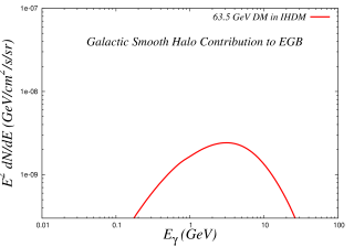
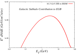
Figure 12: Galactic smooth halo and subhalo contributions to the extragalactic gamma-ray flux for LIP $\sim$ 63.5 GeV dark matter in IHDM. See text for details.

In Fig. 12, we show the contributions to the EGB from both galactic smooth halos and subhalos. From the left panel of Fig. 12 we see that the contribution to the EGB is much subdominant for the annihilation of DM within galactic smooth halo. For our chosen galactic substructure model, this contribution is comparable to that from extragalactic dark matter annihilations calculated using $c_{vir}$ of Macciò et al. model. For the other case where the gamma ray flux from extragalactic dark matter annihilations have been calculated using $c_{vir}$ of power law model, the contributions from the galactic subhalos are much negligible.

6 Summary and Conclusion

We have chosen a simple dark matter (DM) model, namely inert Higgs doublet model (IHDM) where scalar sector of Standard Model is extended by adding another SU(2)_L doublet. The newly added doublet does not generate any VEV after spontaneous symmetry breaking. The ‘inert’ doublet is considered to be the DM candidate. The stability of DM is ensured by imposing discrete $\mathbb{Z}_{2}$ symmetry. The model, in general, provides a broad range of DM mass from GeV to TeV range. In this study we only consider the lower mass range of DM in this model. The analysis of experimental data for DM relic density from PLANCK experiment and the other direct detection experimental results for the case of this IHDM gives a set of best fit values for DM mass, annihilation cross section and other model parameters. We adopt this best fit point (obtained using $\chi^{2}$ minimisation) for IHDM mass from such analyses. Thus the DM mass of $\sim$ 63.5 GeV is our chosen benchmark point in the present work. We study the $\gamma$-ray spectrum obtained from the annihilation of this chosen DM particle in IHDM framework and interpret various types of continuum $\gamma$-ray fluxes with astrophysical origins measured by Fermi-LAT satellite.

In this study we compare our calculated $\gamma$-ray flux with the galactic centre $\gamma$-ray excess in the light of this model. For this we have employed different analysed Fermi-LAT residual $\gamma$-ray flux data for different angular regions around the galactic centre. The calculated low energetic photon spectra from the annihilation of the DM particle with benchmark value of mass ($\sim$ 63.5 GeV) in IHDM for various chosen regions surrounding the galactic centre are found to be in the same ballpark as reported by these studies. Although in some previous analyses it was argued that the photon spectra originated from different annihilation channels of dark matter particles with low masses can possibly fit the obtained data, very recent analyses have obtained the resulting best fit masses of dark matter to be much more conservative (and also somewhat higher as well). We have computed the photon spectra for our benchmark scenario in IHDM framework and have confronted with the residual photon spectra obtained for all of the above-mentioned studies. Our theoretical calculations for photon spectra in this model have been performed after suitable parametrisation of the dark matter halo parameters, region of interest surrounding the galactic centre etc.

We also address the prospects of the continuum $\gamma$-ray signal which may come from DM-dominated dwarf spheroidal galaxies (dSphs) in case they originate from dark matter annihilation. We then compare the $\gamma$-ray flux that can be obtained from the benchmark IHDM dark matter with mass $\sim$ 63.5 GeV. For this we choose 18 Milky Way dSphs whose $J$-factor can be estimated from measurements. The uncertainties in the measurement of $J$-factor for different dSphs are also incorporated in our calculations. The calculated photon spectra for IHDM benchmark point are seen to obey the allowed limits for observed spectra of continuum $\gamma$-ray.

After addressing the issues regarding indirect DM searches with $\gamma$-ray signals from various galactic cases, we finally confront the extragalactic $\gamma$-ray signal with that from the annihilation of low mass DM (considered in this work) in IHDM scenario. We calculate the extragalactic $\gamma$-ray flux for different extragalactic parametrisations and compare with the observed extragalactic gamma ray background by EGRET and Fermi-LAT. For this we consider several possible classes of non-DM astrophysical sources which may yield $\gamma$-ray signal embedded in the extragalactic background. Although there are too many uncertainties involved in modelling of such astrophysical sources and other parameters for extragalactic flux calculation, we have shown that the considered low mass DM in IHDM can generate photon flux within the observed flux limit.

From the detailed study of various galactic and extragalactic $\gamma$-ray searches for probing the indirect signatures of DM in light of IHDM, we can conclude that the low mass DM in this model framework is still a viable candidate to be probed in future $\gamma$-ray searches. Although we have performed the thorough analysis considering only a single Higgs-portal model, the analysis is valid for any simple Higgs-portal DM model such as singlet scalar DM model, singlet fermion DM, inert Higgs triplet model etc. with DM mass in the same ballpark as in our study.

Table 1: Benchmark Point : IHDM Parameters

Model	$M_{h^{0}}$ (GeV)	$M_{H^{\pm}}$ (GeV)	$M_{H^{0}}$ (GeV)	$M_{A^{0}}$ (GeV)	$\lambda_{L}$	$\lambda_{2}$
Parameters	126.016	73.78	63.54	166.16	$-3.29\times 10^{-3}$	$5.67\times 10^{-4}$

Table 2: Benchmark Point : Observables

DM	$\Omega h^{2}$		$\langle\sigma v\rangle$ (cm3s-1)		$\sigma_{\rm SI}$ (pb)
Observables	0.1173		$2.37\times 10^{-26}$		$8.89\times 10^{-11}$
Annihilation	$H^{0}H^{0}\to b\bar{b}$	$H^{0}H^{0}\to W^{+}W^{-}$	$H^{0}H^{0}\to gg$	$H^{0}H^{0}\to l\bar{l}$	$H^{0}H^{0}\to c\bar{c}$	$H^{0}H^{0}\to ZZ$
Cross-section	69.2%	9.61%	9.49%	7.37%	3.29%	0.48%

Table 3: Limits on DM annihilation cross-section from $\gamma$-ray flux limits for various dwarf spheroidal galaxies for the benchmark DM mass of Table 1

dSphs name	longitude	latitude	distance	$\overline{log_{10}({\rm J^{NFW}})}$	$\overline{log_{10}(\alpha_{s}^{\rm NFW})}$	upper limit on
	$l$ ($\deg$)	$b$ ($\deg$)	(kpc)	($log_{10}[{\rm GeV}^{2}{\rm cm}^{-5}{\rm sr}]$)	($log_{10}[\deg]$)	$\langle\sigma v\rangle$ (cm3s-1)
Bootes I	358.1	69.6	66	$18.8\pm 0.22$	$-0.6\pm 0.3$	$2.33\times 10^{-24}$
(Dall’Ora et al., 2006)
Bootes II	353.7	68.9	42	–	–	–
Bootes III	35.4	75.4	47	–	–	–
Canes Venatici I	74.3	79.8	218	$17.7\pm 0.26$	$-1.3\pm 0.2$	$9.65\times 10^{-25}$
(Simon & Geha, 2007)
Canes Venatici II	113.6	82.7	160	$17.9\pm 0.25$	$-1.1\pm 0.4$	$8.14\times 10^{-25}$
(Simon & Geha, 2007)
Canis Major	240.0	-8.0	7	–	–	–
(Walker et al., 2009a)
Carina	260.1	-22.2	105	$18.1\pm 0.23$	$-1.0\pm 0.3$	$2.28\times 10^{-25}$
(Simon & Geha, 2007)
Coma Berenices	241.9	83.6	44	$19.0\pm 0.25$	$-0.6\pm 0.5$	$1.11\times 10^{-24}$
(Simon & Geha, 2007)
Draco	86.4	34.7	76	$18.8\pm 0.16$	$-0.6\pm 0.2$	$3.87\times 10^{-25}$
(Munoz et al., 2005)
Fornax	237.1	-65.7	147	$18.2\pm 0.21$	$-0.8\pm 0.2$	$2.53\times 10^{-25}$
(Walker et al., 2009a)
Hercules	28.7	36.9	132	$18.1\pm 0.25$	$-1.1\pm 0.4$	$9.97\times 10^{-26}$
(Simon & Geha, 2007)
Leo I	226.0	49.1	254	$17.7\pm 0.18$	$-1.1\pm 0.3$	$4.37\times 10^{-25}$
(Mateo et al., 2008)
Leo II	220.2	67.2	233	$17.6\pm 0.18$	$-1.1\pm 0.5$	$3.88\times 10^{-25}$
(Koch et al., 2007)
Leo IV	265.4	56.5	154	$17.9\pm 0.28$	$-1.1\pm 0.4$	$3.72\times 10^{-24}$
(Simon & Geha, 2007)
Leo V	261.9	58.5	178	–	–	–
Pisces II	79.2	-47.1	182	–	–	–
Sagittarius	5.6	-14.2	26	–	–	–
Sculptor	287.5	-83.2	86	$18.6\pm 0.18$	$-0.6\pm 0.3$	$3.41\times 10^{-24}$
(Walker et al., 2009a)
Segue 1	220.5	50.4	23	$19.5\pm 0.29$	$-0.4\pm 0.5$	$1.16\times 10^{-24}$
(Simon et al., 2011)
Segue 2	149.4	-38.1	35	–	–	–
Sextans	243.5	42.3	86	$18.4\pm 0.27$	$-0.9\pm 0.2$	$1.14\times 10^{-25}$
(Walker et al., 2009a)
Ursa Major I	159.4	54.4	97	$18.3\pm 0.24$	$-1.0\pm 0.3$	$1.64\times 10^{-25}$
(Simon & Geha, 2007)
Ursa Major II	152.5	37.4	32	$19.3\pm 0.28$	$-0.5\pm 0.4$	$1.33\times 10^{-24}$
(Simon & Geha, 2007)
Ursa Minor	105.0	44.8	76	$18.8\pm 0.19$	$-0.5\pm 0.2$	$6.54\times 10^{-24}$
(Munoz et al., 2005)
Willman 1	158.6	56.8	38	$19.1\pm 0.31$	$-0.6\pm 0.5$	$4.03\times 10^{-24}$
(Willman et al., 2011)

Table 4: Overview of the minimal non-DM contributions to the total extragalactic $\gamma$-ray background (Tavakoli et al., 2014)

Non-DM objects	Photon Energy Spectra (${dN\over dE}$ in $\textrm{GeV}^{-1}\textrm{cm}^{-2}\textrm{s}^{-1}\textrm{sr}^{-1}$)
BL Lacs	$3.9\times 10^{-8}E_{\gamma}^{-2.23}$
FSRQ	$3.1\times 10^{-8}E_{\gamma}^{-2.45}$
MSP	$1.8\times 10^{-7}E_{\gamma}^{-1.5}\exp\left(-{E_{\gamma}\over 1.9}\right)$
SFG	$1.3\times 10^{-7}E_{\gamma}^{-2.75}$
FR I & FR II	$5.7\times 10^{-8}E_{\gamma}^{-2.39}\exp\left(-{E_{\gamma}\over 50.0}\right)$
UHECR	$4.8\times 10^{-9}E_{\gamma}^{-1.8}\exp\left[-\left({E_{\gamma}\over 100.0}\right)^{0.35}\right]$
GRB	$8.9\times 10^{-9}E_{\gamma}^{-2.1}$
SBG	$0.3\times 10^{-7}E_{\gamma}^{-2.4}$
UHEp ICM	$3.1\times 10^{-9}E_{\gamma}^{-2.75}$
IGS	$0.87\times 10^{-10}\times\left\{\begin{array}[]{ll}&\left(\frac{E_{\gamma}}{10}\right)^{-2.04}\;\textrm{for}\;E_{\gamma}<10\ \textrm{GeV}\\ &\left(\frac{E_{\gamma}}{10}\right)^{-2.13}\;\textrm{for}\;E_{\gamma}>10\ \textrm{GeV}\end{array}\right\}$

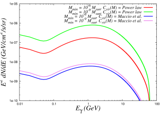
Figure 9: Comparison of the computed extragalactic gamma-ray fluxes from the annihilation of $\sim$ 63.5 GeV dark matter (benchmark point) in IHDM framework for different extragalactic parametrisations. We consider two models of the concentration parameter $c_{vir}$, namely a)power law model and b)Macciò et al. model. Also the minimum extragalactic subhalo mass $M_{\rm min}$ are chosen to be $10^{-6}M_{\odot}\,\,{\rm and}\,\,10^{-9}\,M_{\odot}$. Calculation with power law model yields enhanced $\gamma$-ray flux compared to that with Macciò et al. model. For low $M_{\rm min}$, $\gamma$-ray flux increases and this enhancement is smaller for Macciò et al. model compared to that for power law model. See text for details.

References

- Aalseth et al. (2011) Aalseth, C., et al. 2011, Phys.Rev.Lett., 106, 131301
- Abdo et al. (2010a) Abdo, A., et al. 2010a, Astrophys.J., 712, 147
- Abdo et al. (2010b) —. 2010b, Phys.Rev.Lett., 104, 101101
- Abdullah et al. (2014) Abdullah, M., DiFranzo, A., Rajaraman, A., et al. 2014, Phys.Rev., D90, 035004
- Ackermann et al. (2011) Ackermann, M., et al. 2011, Phys.Rev.Lett., 107, 241302
- Ackermann et al. (2014) —. 2014, Phys.Rev., D89, 042001
- Ackermann et al. (2015a) —. 2015a, arXiv:1501.05464
- Ackermann et al. (2015b) —. 2015b, Astrophys.J., 799, 86
- Ade et al. (2014) Ade, P., et al. 2014, Astron.Astrophys., 571, A16
- Agashe et al. (2014) Agashe, K., Cui, Y., Necib, L., & Thaler, J. 2014, JCAP, 1410, 062
- Agnese et al. (2013a) Agnese, R., et al. 2013a, Phys.Rev.Lett., 111, 251301
- Agnese et al. (2013b) —. 2013b, Phys.Rev., D88, 031104
- Agrawal et al. (2014a) Agrawal, P., Batell, B., Fox, P. J., & Harnik, R. 2014a, arXiv:1411.2592
- Agrawal et al. (2014b) Agrawal, P., Batell, B., Hooper, D., & Lin, T. 2014b, Phys.Rev., D90, 063512
- Agrawal et al. (2014c) Agrawal, P., Blanke, M., & Gemmler, K. 2014c, JHEP, 1410, 72
- Agrawal et al. (2009) Agrawal, P., Dolle, E. M., & Krenke, C. A. 2009, Phys.Rev., D79, 015015
- Ahmed et al. (2010) Ahmed, Z., et al. 2010, Science, 327, 1619
- Ajello et al. (2015) Ajello, M., Gasparrini, D., Sánchez-Conde, M., et al. 2015, Astrophys.J., 800, L27
- Akerib et al. (2014) Akerib, D., et al. 2014, Phys.Rev.Lett., 112, 091303
- Alves et al. (2014) Alves, A., Profumo, S., Queiroz, F. S., & Shepherd, W. 2014, Phys.Rev., D90, 115003
- Anchordoqui & Vlcek (2013) Anchordoqui, L. A., & Vlcek, B. J. 2013, Phys.Rev., D88, 043513
- Ando (2005) Ando, S. 2005, Phys.Rev.Lett., 94, 171303
- Ando (2009) —. 2009, Phys.Rev., D80, 023520
- Ando & Komatsu (2013) Ando, S., & Komatsu, E. 2013, Phys.Rev., D87, 123539
- Andreas et al. (2009) Andreas, S., Tytgat, M. H., & Swillens, Q. 2009, JCAP, 0904, 004
- Angloher et al. (2012) Angloher, G., Bauer, M., Bavykina, I., et al. 2012, Eur.Phys.J., C72, 1971
- Aprile (2013) Aprile, E. 2013, Springer Proc.Phys., C12-02-22, 93
- Aprile et al. (2011) Aprile, E., et al. 2011, Phys.Rev.Lett., 107, 131302
- Aprile et al. (2012) —. 2012, Phys.Rev.Lett., 109, 181301
- Arhrib et al. (2012) Arhrib, A., Benbrik, R., & Gaur, N. 2012, Phys.Rev., D85, 095021
- Arhrib et al. (2014) Arhrib, A., Tsai, Y.-L. S., Yuan, Q., & Yuan, T.-C. 2014, JCAP, 1406, 030
- Arina et al. (2015) Arina, C., Del Nobile, E., & Panci, P. 2015, Phys.Rev.Lett., 114, 011301
- Arina et al. (2009) Arina, C., Ling, F.-S., & Tytgat, M. H. 2009, JCAP, 0910, 018
- Atwood et al. (2009) Atwood, W., et al. 2009, Astrophys.J., 697, 1071
- Balázs & Li (2014) Balázs, C., & Li, T. 2014, Phys.Rev., D90, 055026
- Banik & Majumdar (2014) Banik, A. D., & Majumdar, D. 2014, arXiv:1408.5795
- Barger et al. (2008) Barger, V., Langacker, P., McCaskey, M., Ramsey-Musolf, M. J., & Shaughnessy, G. 2008, Phys.Rev., D77, 035005
- Basak & Mondal (2014) Basak, T., & Mondal, T. 2014, arXiv:1405.4877
- Battaglia et al. (2013) Battaglia, G., Helmi, A., & Breddels, M. 2013, New Astron.Rev., 57, 52
- Begeman et al. (1991) Begeman, K., Broeils, A., & Sanders, R. 1991, Mon.Not.Roy.Astron.Soc., 249, 523
- Belanger et al. (2011) Belanger, G., Boudjema, F., Brun, P., et al. 2011, Comput.Phys.Commun., 182, 842
- Belanger et al. (2014) Belanger, G., Boudjema, F., Pukhov, A., & Semenov, A. 2014, Comput.Phys.Commun., 185, 960
- Bell et al. (2015) Bell, N. F., Horiuchi, S., & Shoemaker, I. M. 2015, Phys.Rev., D91, 023505
- Bergstrom et al. (2001) Bergstrom, L., Edsjo, J., & Ullio, P. 2001, Phys.Rev.Lett., 87, 251301
- Berlin et al. (2014a) Berlin, A., Gratia, P., Hooper, D., & McDermott, S. D. 2014a, Phys.Rev., D90, 015032
- Berlin et al. (2014b) Berlin, A., Hooper, D., & McDermott, S. D. 2014b, Phys.Rev., D89, 115022
- Boehm et al. (2014a) Boehm, C., Dolan, M. J., & McCabe, C. 2014a, Phys.Rev., D90, 023531
- Boehm et al. (2014b) Boehm, C., Dolan, M. J., McCabe, C., Spannowsky, M., & Wallace, C. J. 2014b, JCAP, 1405, 009
- Borah & Dasgupta (2015) Borah, D., & Dasgupta, A. 2015, Phys.Lett., B741, 103
- Boucenna & Profumo (2011) Boucenna, M., & Profumo, S. 2011, Phys.Rev., D84, 055011
- Branco et al. (2012) Branco, G., Ferreira, P., Lavoura, L., et al. 2012, Phys.Rept., 516, 1
- Bringmann (2009) Bringmann, T. 2009, New J.Phys., 11, 105027
- Bringmann et al. (2014) Bringmann, T., Calore, F., Di Mauro, M., & Donato, F. 2014, Phys.Rev., D89, 023012
- Bryan & Norman (1998) Bryan, G., & Norman, M. 1998, Astrophys.J., 495, 80
- Buckley et al. (2013) Buckley, M. R., Hooper, D., & Kumar, J. 2013, Phys.Rev., D88, 063532
- Buckley et al. (2011a) Buckley, M. R., Hooper, D., & Rosner, J. L. 2011a, Phys.Lett., B703, 343
- Buckley et al. (2011b) Buckley, M. R., Hooper, D., & Tait, T. M. 2011b, Phys.Lett., B702, 216
- Burgess et al. (2001) Burgess, C., Pospelov, M., & ter Veldhuis, T. 2001, Nucl.Phys., B619, 709
- Cahill-Rowley et al. (2015) Cahill-Rowley, M., Gainer, J., Hewett, J., & Rizzo, T. 2015, JHEP, 1502, 057
- Calore et al. (2014a) Calore, F., Cholis, I., McCabe, C., & Weniger, C. 2014a, arXiv:1411.4647
- Calore et al. (2014b) Calore, F., Cholis, I., & Weniger, C. 2014b, arXiv:1409.0042
- Cao et al. (2014) Cao, J., Shang, L., Wu, P., Yang, J. M., & Zhang, Y. 2014, arXiv:1410.3239
- Cao et al. (2007) Cao, Q.-H., Ma, E., & Rajasekaran, G. 2007, Phys.Rev., D76, 095011
- Cerdeno et al. (2015) Cerdeno, D., Peiro, M., & Robles, S. 2015, arXiv:1501.01296
- Cerdeño et al. (2014) Cerdeño, D., Peiró, M., & Robles, S. 2014, JCAP, 1408, 005
- Chang & Ng (2014) Chang, W.-F., & Ng, J. N. 2014, Phys.Rev., D90, 065034
- Cheng et al. (2002) Cheng, H.-C., Feng, J. L., & Matchev, K. T. 2002, Phys.Rev.Lett., 89, 211301
- Cheung et al. (2014) Cheung, C., Papucci, M., Sanford, D., Shah, N. R., & Zurek, K. M. 2014, Phys.Rev., D90, 075011
- Cholis et al. (2014) Cholis, I., Hooper, D., & McDermott, S. D. 2014, JCAP, 1402, 014
- Cirelli et al. (2011) Cirelli, M., Corcella, G., Hektor, A., et al. 2011, JCAP, 1103, 051
- Cline et al. (2014) Cline, J. M., Dupuis, G., Liu, Z., & Xue, W. 2014, JHEP, 1408, 131
- Dall’Ora et al. (2006) Dall’Ora, M., Clementini, G., Kinemuchi, K., et al. 2006, Astrophys.J., 653, L109
- Daylan et al. (2014) Daylan, T., Finkbeiner, D. P., Hooper, D., et al. 2014, arXiv:1402.6703
- Deshpande & Ma (1978) Deshpande, N. G., & Ma, E. 1978, Phys.Rev., D18, 2574
- Detmold et al. (2014) Detmold, W., McCullough, M., & Pochinsky, A. 2014, Phys.Rev., D90, 115013
- Di Mauro (2015) Di Mauro, M. 2015, arXiv:1502.02566
- Di Mauro & Donato (2015) Di Mauro, M., & Donato, F. 2015, arXiv:1501.05316
- Diemand et al. (2007) Diemand, J., Kuhlen, M., & Madau, P. 2007, Astrophys.J., 667, 859
- Djouadi et al. (2012) Djouadi, A., Lebedev, O., Mambrini, Y., & Quevillon, J. 2012, Phys.Lett., B709, 65
- Dolle et al. (2010) Dolle, E., Miao, X., Su, S., & Thomas, B. 2010, Phys.Rev., D81, 035003
- Dolle & Su (2009) Dolle, E. M., & Su, S. 2009, Phys.Rev., D80, 055012
- Dominguez et al. (2011) Dominguez, A., Primack, J., Rosario, D., et al. 2011, Mon.Not.Roy.Astron.Soc., 410, 2556
- Duffy & van Bibber (2009) Duffy, L. D., & van Bibber, K. 2009, New J.Phys., 11, 105008
- Fermi-LAT Collaboration (2012) Fermi-LAT Collaboration. 2012, Astrophys.J.Suppl., 199, 31
- Fermi-LAT Collaboration (2015) —. 2015, arXiv:1501.02003
- Fichtel et al. (1978) Fichtel, C. E., Simpson, G. A., & Thompson, D. J. 1978, ApJ, 222, 833
- Fields et al. (2014) Fields, B. D., Shapiro, S. L., & Shelton, J. 2014, Phys.Rev.Lett., 113, 151302
- Franceschini et al. (2008) Franceschini, A., Rodighiero, G., & Vaccari, M. 2008, Astron.Astrophys., 487, 837
- Freytsis et al. (2015) Freytsis, M., Robinson, D. J., & Tsai, Y. 2015, Phys.Rev., D91, 035028
- Gao et al. (1991) Gao, Y.-T., Stecker, F. W., & Cline, D. B. 1991, Astron.Astrophys., 249, 1
- Geringer-Sameth & Koushiappas (2011) Geringer-Sameth, A., & Koushiappas, S. M. 2011, Phys.Rev.Lett., 107, 241303
- Geringer-Sameth & Koushiappas (2012) —. 2012, Phys.Rev., D86, 021302
- Ghorbani & Ghorbani (2014) Ghorbani, K., & Ghorbani, H. 2014, arXiv:1501.00206
- Ghosh et al. (2015) Ghosh, D. K., Mondal, S., & Saha, I. 2015, JCAP, 1502, 035
- Gonderinger et al. (2010) Gonderinger, M., Li, Y., Patel, H., & Ramsey-Musolf, M. J. 2010, JHEP, 1001, 053
- Goudelis et al. (2013) Goudelis, A., Herrmann, B., & Stål, O. 2013, JHEP, 1309, 106
- Guo et al. (2014) Guo, J., Li, J., Li, T., & Williams, A. G. 2014, arXiv:1409.7864
- Gustafsson et al. (2012) Gustafsson, M., Rydbeck, S., Lopez-Honorez, L., & Lundstrom, E. 2012, Phys.Rev., D86, 075019
- Hambye et al. (2009) Hambye, T., Ling, F.-S., Lopez Honorez, L., & Rocher, J. 2009, JHEP, 0907, 090
- Hambye & Tytgat (2008) Hambye, T., & Tytgat, M. H. 2008, Phys.Lett., B659, 651
- Heikinheimo & Spethmann (2014) Heikinheimo, M., & Spethmann, C. 2014, JHEP, 1412, 084
- Hooper (2012) Hooper, D. 2012, Phys.Dark Univ., 1, 1
- Hooper & Linden (2011) Hooper, D., & Linden, T. 2011, Phys.Rev., D84, 123005
- Hooper & Slatyer (2013) Hooper, D., & Slatyer, T. R. 2013, Phys.Dark Univ., 2, 118
- Hooper et al. (2012) Hooper, D., Weiner, N., & Xue, W. 2012, Phys.Rev., D86, 056009
- Huang et al. (2014) Huang, J., Liu, T., Wang, L.-T., & Yu, F. 2014, Phys.Rev., D90, 115006
- Huang et al. (2013) Huang, W.-C., Urbano, A., & Xue, W. 2013, arXiv:1307.6862
- Ipek et al. (2014) Ipek, S., McKeen, D., & Nelson, A. E. 2014, Phys.Rev., D90, 055021
- Izaguirre et al. (2014) Izaguirre, E., Krnjaic, G., & Shuve, B. 2014, Phys.Rev., D90, 055002
- Jenkins et al. (1998) Jenkins, A., et al. 1998, Astrophys.J., 499, 20
- Kanemura et al. (2010) Kanemura, S., Matsumoto, S., Nabeshima, T., & Okada, N. 2010, Phys.Rev., D82, 055026
- Kanemura et al. (2011) Kanemura, S., Okada, Y., Taniguchi, H., & Tsumura, K. 2011, Phys.Lett., B704, 303
- Kim et al. (2008) Kim, Y. G., Lee, K. Y., & Shin, S. 2008, JHEP, 0805, 100
- Klypin et al. (2002) Klypin, A., Zhao, H., & Somerville, R. S. 2002, Astrophys.J., 573, 597
- Ko et al. (2014) Ko, P., Park, W.-I., & Tang, Y. 2014, JCAP, 1409, 013
- Ko & Tang (2015) Ko, P., & Tang, Y. 2015, JCAP, 1501, 023
- Koch et al. (2007) Koch, A., Kleyna, J., Wilkinson, M., et al. 2007, Astron.J., 134, 566
- Komatsu et al. (2011) Komatsu, E., et al. 2011, Astrophys.J.Suppl., 192, 18
- Krawczyk et al. (2013) Krawczyk, M., Sokolowska, D., Swaczyna, P., & Swiezewska, B. 2013, JHEP, 1309, 055
- Kuhlen et al. (2008) Kuhlen, M., Diemand, J., & Madau, P. 2008, Astrophys.J., 686, 262
- Lacroix et al. (2014) Lacroix, T., Boehm, C., & Silk, J. 2014, Phys.Rev., D90, 043508
- Lebedev et al. (2012) Lebedev, O., Lee, H. M., & Mambrini, Y. 2012, Phys.Lett., B707, 570
- Logan (2011) Logan, H. E. 2011, Phys.Rev., D83, 035022
- Lopez Honorez & Yaguna (2010) Lopez Honorez, L., & Yaguna, C. E. 2010, JHEP, 1009, 046
- Lopez Honorez & Yaguna (2011) —. 2011, JCAP, 1101, 002
- Lundstrom et al. (2009) Lundstrom, E., Gustafsson, M., & Edsjo, J. 2009, Phys.Rev., D79, 035013
- Ma (2006) Ma, E. 2006, Phys.Rev., D73, 077301
- Maccio’ et al. (2008) Maccio’, A. V., Dutton, A. A., & Bosch, F. C. d. 2008, Mon.Not.Roy.Astron.Soc., 391, 1940
- Marshall & Primulando (2011) Marshall, G., & Primulando, R. 2011, JHEP, 1105, 026
- Martin et al. (2014) Martin, A., Shelton, J., & Unwin, J. 2014, Phys.Rev., D90, 103513
- Martinez (2013) Martinez, G. D. 2013, arXiv:1309.2641
- Martinez et al. (2009) Martinez, G. D., Bullock, J. S., Kaplinghat, M., Strigari, L. E., & Trotta, R. 2009, JCAP, 0906, 014
- Massey et al. (2007) Massey, R., Rhodes, J., Ellis, R., et al. 2007, Nature, 445, 286
- Mateo et al. (2008) Mateo, M., Olszewski, E. W., & Walker, M. G. 2008, Astrophys.J., 675, 201
- Mazziotta et al. (2012) Mazziotta, M., Loparco, F., de Palma, F., & Giglietto, N. 2012, Astropart.Phys., 37, 26
- Melfo et al. (2011) Melfo, A., Nemevsek, M., Nesti, F., Senjanovic, G., & Zhang, Y. 2011, Phys.Rev., D84, 034009
- Modak (2014) Modak, K. P. 2014, arXiv:1404.3676
- Modak & Majumdar (2013) Modak, K. P., & Majumdar, D. 2013, J.Phys., G40, 075201
- Modak et al. (2013) Modak, K. P., Majumdar, D., & Rakshit, S. 2013, arXiv:1312.7488
- Munoz et al. (2005) Munoz, R. R., Frinchaboy, P. M., Majewski, S. R., et al. 2005, Astrophys.J., 631, L137
- Murgia (2014) Murgia, S. 2014, Fifth International Fermi Symposium http://fermi.gsfc.nasa.gov/science/mtgs/symposia/2014/program/08_Murgia%.pdf
- Murray et al. (2013) Murray, S., Power, C., & Robotham, A. 2013, arXiv:1306.6721
- Navarro et al. (1996) Navarro, J. F., Frenk, C. S., & White, S. D. 1996, Astrophys.J., 462, 563
- Navarro et al. (1997) —. 1997, Astrophys.J., 490, 493
- Neto et al. (2007) Neto, A. F., Gao, L., Bett, P., et al. 2007, Mon.Not.Roy.Astron.Soc., 381, 1450
- Nezri et al. (2009) Nezri, E., Tytgat, M. H., & Vertongen, G. 2009, JCAP, 0904, 014
- Ng et al. (2014) Ng, K. C. Y., Laha, R., Campbell, S., et al. 2014, Phys.Rev., D89, 083001
- Oda et al. (2005) Oda, T., Totani, T., & Nagashima, M. 2005, Astrophys.J., 633, L65
- Okada & Seto (2014a) Okada, N., & Seto, O. 2014a, Phys.Rev., D90, 083523
- Okada & Seto (2014b) —. 2014b, Phys.Rev., D89, 043525
- Pieri et al. (2008) Pieri, L., Bertone, G., & Branchini, E. 2008, Mon.Not.Roy.Astron.Soc., 384, 1627
- Press & Schechter (1974) Press, W. H., & Schechter, P. 1974, Astrophys.J., 187, 425
- Randall & Sundrum (1999) Randall, L., & Sundrum, R. 1999, Nucl.Phys., B557, 79
- Sefusatti et al. (2014) Sefusatti, E., Zaharijas, G., Serpico, P. D., Theurel, D., & Gustafsson, M. 2014, Mon.Not.Roy.Astron.Soc., 441, 1861
- Servant & Tait (2003) Servant, G., & Tait, T. M. 2003, Nucl.Phys., B650, 391
- Sheth & Tormen (1999) Sheth, R. K., & Tormen, G. 1999, Mon.Not.Roy.Astron.Soc., 308, 119
- Sheth & Tormen (2004) —. 2004, Mon.Not.Roy.Astron.Soc., 350, 1385
- Silveira & Zee (1985) Silveira, V., & Zee, A. 1985, Phys.Lett., B161, 136
- Simon & Geha (2007) Simon, J. D., & Geha, M. 2007, Astrophys.J., 670, 313
- Simon et al. (2011) Simon, J. D., Geha, M., Minor, Q. E., et al. 2011, Astrophys.J., 733, 46
- Springel et al. (2008a) Springel, V., Wang, J., Vogelsberger, M., et al. 2008a, Mon.Not.Roy.Astron.Soc., 391, 1685
- Springel et al. (2008b) Springel, V., White, S., Frenk, C., et al. 2008b, Nature, 456N7218, 73
- Sreekumar et al. (1998) Sreekumar, P., et al. 1998, Astrophys.J., 494, 523
- Stecker (1978) Stecker, F. 1978, Astrophys.J., 223, 1032
- Strigari (2013) Strigari, L. E. 2013, Phys.Rept., 531, 1
- Swiezewska & Krawczyk (2013a) Swiezewska, B., & Krawczyk, M. 2013a, 563
- Swiezewska & Krawczyk (2013b) —. 2013b, Phys.Rev., D88, 035019
- Tavakoli et al. (2014) Tavakoli, M., Cholis, I., Evoli, C., & Ullio, P. 2014, JCAP, 1401, 017
- Taylor & Silk (2003) Taylor, J. E., & Silk, J. 2003, Mon.Not.Roy.Astron.Soc., 339, 505
- Ullio et al. (2002) Ullio, P., Bergstrom, L., Edsjo, J., & Lacey, C. G. 2002, Phys.Rev., D66, 123502
- Veltman & Yndurain (1989) Veltman, M., & Yndurain, F. 1989, Nucl.Phys., B325, 1
- Walker et al. (2009a) Walker, M. G., Mateo, M., & Olszewski, E. 2009a, Astron.J., 137, 3100
- Walker et al. (2009b) Walker, M. G., Mateo, M., Olszewski, E. W., et al. 2009b, Astrophys.J., 704, 1274
- Wang & Han (2014) Wang, L., & Han, X.-F. 2014, Phys.Lett., B739, 416
- Willman et al. (2011) Willman, B., Geha, M., Strader, J., et al. 2011, Astron.J., 142, 128
- Wolf et al. (2010) Wolf, J., Martinez, G. D., Bullock, J. S., et al. 2010, Mon.Not.Roy.Astron.Soc., 406, 1220
- Yu (2014) Yu, J.-H. 2014, Phys.Rev., D90, 095010
- Zhu (2011) Zhu, G. 2011, Phys.Rev., D83, 076011