Excitonic Spectra of Wide Parabolic Quantum Wells

Abstract

The optical properties of wide Quantum Wells are considered, taking into account the screened electron-hole interaction potential and parabolic confinement potentials, different for the electrons and for the holes. The role of the interaction potential which mixes the energy states according to different quantum numbers is stressed. The results obtained by our method are in agreement with the observed spectra and give the possibility to the assessment of the resonances.

1 Introduction

A single Quantum Well (QW) is formed when a thin layer of a narrow gap semiconductor material (Well) lies between layers of wider gap materials (Barriers). The size of QWs (taken in the growth direction) is generally between 1 and 20 nm (narrow QWs). Mostly the size is comparable with the effective excitonic Bohr radius $a^{*}$ of the QW material (for example, $a^{*}$ is about 10 nm for GaAs). When the size of the QW is of the order of a few excitonic Bohr radii, we speak about Wide Quantum Well (50-100 nm in the case of GaAs Wells). Typical property of the QWs is the confinement of the carriers (electrons and holes) inside the well. Mostly one considers a rectangular shape of the confinement potential, but also other shapes are considered. A special fabrication technique allows to create a parabolic shaped confinement, leading to the so-called Parabolic Quantum Wells (PQWs). More generally, we can speak about Parabolic Quantum Nanostructures (for example, Parabolic Quantum Dots). When the size of a PQW corresponds to the Wide QW region, we deal with Wide Parabolic Quantum Wells (WPQWs). The structures with parabolic confinement have attracted more attention in the recent decades (for example, Ref. [1]-[15]).

Each type of semiconductor structures has a specific property depending on its dimensionality, which influences the optical characteristic of a given structure. In bulk crystals the coupling between the external electromagnetic wave and the internal polariton modes gives rise to the so-called ABC problem, which was extensively examined in the past [16]-[25]). In low-dimensional structures as Quantum Wells, Quantum Wires and Quantum Dots mostly the long-wave approximation is used, so the electrodynamical aspect is simplified, however, on the other hand, due to the confinement, the separation of center-of-mass and relative e-h motion is not possible and the problem of solving 6-dimensional Schrödinger equation appears. The additional difficulty consists on the fact that the spherical symmetry of the Coulomb potential is not compatible with the cylindrical symmetry of most nanostructures. Thus several approximations have been proposed which used the lowering of the dimension of the problem (for example, [26]). Recently, also due to the increasing power of computers, direct numerical solution of the 6-dimensional 2-particles Schrödinger equation has been performed (for example, Refs. [27], [28]).

Here we consider Wide Quantum Wells (WQWs), nanostructures where the optical active layers have extension of a few excitonic Bohr radii in the growth direction. To a certain approximation, the polaritonic aspect can be here neglected, and the long-wave approximation sustained. The exciton is not squeezed as in other low-dimensional structures. In typical Quantum Wells with the dimension of, say, one excitonic Bohr radius in the growth direction we observe only a few excited states. In WQWs, due to the greater extension, significantly larger number of states is observed. The Coulomb potential and different confinement potentials for electrons and holes couples electron and hole confinement states of different quantum numbers. Such phenomena have been observed experimentally (see, for example, Ref. [1]). We propose the computational method which leads to analytical expression for the electric susceptibility of wide parabolic quantum well taking into account the screened electron-hole interaction and parabolic confinement potential. With the purpose of exemplification, we consider a quantum well with GaAs as the optically active layer and Ga_1-xAl_xAs as the barriers, where the active layer is of the extension of a few excitonic Bohr radii. The absorption spectra of such a structure show a large number of resonances ($n=8$ observed in [1]). The choice of optimal effective potential parameters as well as the damping constant used in our calculation is verified by numerical calculations of the total fitting error for maxima of susceptibility. We have chosen as reference the paper by Miller et al [1] because it contains a lot of experimental data which allowed to compare the obtained theoretical results with experiment. The agreement between our calculated spectrum and experimental data is very good with regard to the number and position of the maxima of susceptibility.

Our paper is organized as follows. In the section 2, we present the assumptions of considered model and solve the constitutive equation with effective electron-hole interaction potential. Section 3 is devoted to the details of the applied potential. Next, in section 4, the derived solution of constitutive equation is used to obtain the energy levels of the considered GaAs/Ga_1-xAl_xAs wide parabolic quantum well. Finally, in section 5, the susceptibility for such nanostructure is calculated and discussed. The comparison of obtained results with experimental data and a brief overview of optimizing procedure is included.

2 The Model

We will compute the linear optical response of a WPQW to a plain electromagnetic wave

$$E_{i}(z,t)=E_{i0}\exp({\rm i}k_{0}z-{\rm i}\omega t),\qquad k_{0}=\frac{\omega}{c},$$ (1)

attaining the boundary surface of the WPQQW active layer located at the plane $z=0$. The second boundary is located at the plane $z=L$. In the case of GaAs Well the extension $L$ will be of the order 2-40 nm.

Due to this extension, the following aspects should be taken into account. 1) Several confinement states resulting from the confinement in the $z$ direction are to be included in the consideration. 2) The electron-hole potential plays an important role and cannot be approximated by a 2-dimensional potential, as was sometimes done in the case of simple Quantum Wells (the limit $L\rightarrow 0$). 3) The parabolic shape of the confinement potential is assumed

$$V_{\rm uw}(z_{e},z_{h})=\frac{1}{2}m_{ez}\omega_{e}^{2}z_{e}^{2}+\frac{1}{2}m_{hz}\omega_{h}^{2}z_{h}^{2}.$$ (2)

4) The electron-hole interaction is described by the potential $V({\bf r}_{e},{\bf r}_{h})$. 5) We adopt the real density matrix approach to compute the optical properties. In this approach the linear optical response will be described by a set of coupled equations: two constitutive equations for the coherent amplitudes $Y_{\nu}(\textbf{r}_{e},\textbf{r}_{h})$, $\nu=\hbox{H,L}$ stands for heavy-hole (H) and light-hole exciton); from them the polarization can be obtained and used in Maxwell’s field equations. Having the field we can determine the QW optical functions (reflectivity, transmission, and absorption).

Thus the next steps are the following: We formulate the constitutive equations. The equations will be then solved giving the coherent amplitudes $Y$. From the amplitudes we compute the polarization inside the Quantum Well, the electric field of the wave, and the optical functions. This scheme will be applied for the case investigated in Ref. [1].

As was explained in, for example, Ref. [24], the constitutive equation for the coherent amplitude $Y$ in a Quantum Well has the form

$$\left[E_{g}-\hbar\omega-{\rm i}{\mit\Gamma}+\frac{\hat{p}_{ez}^{2}}{2m_{e}}+\frac{\hat{p}_{hz}^{2}}{2m_{hz}}+\frac{\hat{\bf p}_{\rho}^{2}}{2\mu_{\parallel}}+\frac{\hat{\bf p}_{\parallel}^{2}}{2M_{\parallel}}+V_{eh}(\rho,z_{e},z_{h})+V_{\rm conf}(z_{e},z_{h})\right]Y={\bf M}({\bf r}){\bf E}({\bf R}),$$ (3)

where ${\bf M}({\bf r})$ is the transition dipole density, which form we have assumed as

$${\bf M}({\bf r})={\bf M}(\rho,z,\phi)=\frac{\textbf{M}_{0}}{2\pi\rho_{0}}\delta(z)\delta\left(\rho-\rho_{0}\right),$$ (4)

$z=z_{e}-z_{h}$ being the relative coordinate in the $z$ direction, $\rho_{0}$ is the coherence radius, ${\bf R}$ jest is the excitonic center-of-mass coordinate and ${\bf E}({\bf R})$ is the electric field vector of the wave propagating in the QW; $V_{\rm conf}(z_{e},z_{h})$ is the confinement potential for electrons and holes, and $\hat{\bf p}_{\rho}$, $\hat{\bf p}_{\parallel}$ are the momentum operators for the excitonic relative- and center-of-mass motion in the QW plane.

In the following we assume that the propagating wave is linearly polarized in the $x$ direction, and that the vector M has a non-vanishing component in the same direction. Taking the confinement potential in the form (2) we find in the equation (3) Hamilton operators for the one-dimensional harmonic oscillator

$$H_{e}=\frac{\hat{p}_{ez}^{2}}{2m_{e}}+\frac{1}{2}m_{e}\omega_{e}^{2}z_{e}^{2},\,\,\,\,\,\,H_{h}=\frac{\hat{p}_{hz}^{2}}{2m_{h}}+\frac{1}{2}m_{h}\omega_{h}^{2}z_{h}^{2}.$$ (5)

Therefore we look for a solutions $Y$ in terms of the eigenfunctions of the operators $H_{e},H_{h}$

$$Y\left(\rho,z_{e},z_{h}\right)=\sum\limits_{j,n=0}^{N}\psi_{ej}(z_{e})\psi_{nh}(z_{h})Y_{jn}(\hbox{\boldmath$\rho$}),$$ (6)

The eigenfunctions $\psi_{j}$ have the form

$$\psi_{ej}(z_{e}) = \pi^{-1/4}\sqrt{\frac{\alpha_{e}}{2^{j}j!}}H_{j}\left(\alpha_{e}z_{e}\right)e^{-\frac{\alpha_{e}^{2}}{2}z_{e}^{2}};\qquad\alpha_{e}=\sqrt{\frac{m_{ez}\omega_{e}}{\hbar}},$$

$$\psi_{nh}(z_{h}) = \pi^{-1/4}\sqrt{\frac{\alpha_{h}}{2^{n}n!}}H_{n}\left(\alpha_{h}z_{h}\right)e^{-\frac{\alpha_{h}^{2}}{2}z_{h}^{2}};\qquad\alpha_{h}=\sqrt{\frac{m_{hz}\omega_{h}}{\hbar}},$$ (7)

with the Hermite polynomials $H_{n}(x)$, and the corresponding eigenvalues $E_{n}=\left(n+\frac{1}{2}\right)\hbar\omega$. Substituting (6) into the eq. (3) we obtain equations for the functions $Y_{jn}$

$$\sum\limits_{j,n=0}^{N}\left[E_{g}-\hbar\omega-{\rm i}{\mit\Gamma}+E_{je}+E_{nh}+\frac{\hat{\bf p}_{\hbox{\boldmath$\rho$}}^{2}}{2\mu_{\parallel}}+\frac{\hat{\bf p}_{\parallel}^{2}}{2M_{\parallel}}+V_{eh}(\hbox{\boldmath$\rho$},z_{e},z_{h})\right]\psi_{j}(z_{e})\psi_{n}(z_{h})Y_{jn}(\hbox{\boldmath$\rho$})={\bf M}({\bf r}){\bf E}({\bf R}).$$

Now we have to specify the shape of the interaction potential $V_{eh}(\hbox{\boldmath$\rho$},z_{e},z_{h})$ and the wave electric field ${\bf E}({\bf R})$. We assume the so-called long-wave approximation and consider ${\bf E}({\bf R})$ in the equation (2) as a constant quantity.The electron-hole interaction potential $V_{eh}(\hbox{\boldmath$\rho$},z_{e},z_{h})$ is, in general, the screened Coulomb potential

$$V_{eh}(\rho,z_{e},z_{h})=-\frac{e^{2}}{4\pi\epsilon_{b}\sqrt{\rho^{2}+\left(z_{e}-z_{h}\right)^{2}}},$$ (9)

$\epsilon_{b}$ being the dielectric constant of the QW material. Despite of the nanostructures with cylindrical symmetry considered in ref.[28], in the case of the wide QWs one does not have an orthonormal basis of functions so the use of an effective e-h interaction potential will be made

$$V_{eh}=-S\exp\left[-v\left(z_{e}-z_{h}\right)^{2}-w\rho^{2}\right].$$ (10)

where $v,w$ are certain parameters which will be estimated below. Using the above potential, the dipole density (4), and neglecting the center-of-mass in plane motion, we put the constitutive equation (3) into the form

$$\left(E_{rs}+\frac{\hat{\bf p}_{\hbox{\boldmath$\rho$}}^{2}}{2\mu_{\parallel}}\right)Y_{rs}-e^{-w\rho^{2}}\sum\limits_{nj}V_{rsnj}Y_{nj}=E\frac{M_{0}}{2\pi\rho_{0}}\langle r|s\rangle\delta\left(\rho-\rho_{0}\right),$$ (11)

where

$$E_{rs} = E_{g}+E_{re}+E_{sh}-\hbar\omega-{\rm i}{\mit\Gamma},\qquad r,s,=0,1,2,\ldots\,,$$

$$V_{rsnj} = S\langle rs\left|\exp\left[-v\left(z_{e}-z_{h}\right)^{2}\right]\right|nj\rangle$$ (12)

With regard to the shape of the functions $\psi$ only states of the same parity will give nonvanishing elements $\langle r|s\rangle$ so the states $|0e0h\rangle,|0e2h\rangle,|1e3h\rangle$ etc. will be taken into account. To summarize in order to calculate the optical response of a wide Quantum Well it is necessery to solve the constitutive equation (11) using the matrix elements $\langle r|s\rangle$ and the potential matrix elements (12).

3 The parameters of the effective potential

The further calculations require the estimation of parameters characterizing the effective potential (10). We make the following assumptions: 1) The potential is isotropic, in analogy to the Coulomb potential in isotropic materials. The nanostructure anisotropy is included in the quasiparticles effective masses. This assumption leads to the equality $u=v$. 2) We assume the value $S\approx 2R^{*}$ ($R^{*}$ being the effective excitonic Rydberg energy for the given crystal); the exact value $S$ will be established later. We determine the ground state energy of a hydrogen-like atom, where the interaction between the charges is given by (10). To this end we solve the Schrödinger equation

$$-\frac{\hbar^{2}}{2\mu}\left(\frac{{\rm d}^{2}}{{\rm d}r^{2}}+\frac{2}{r}\frac{\partial}{\partial r}\right)\psi-SR^{*}e^{-vr^{2}}\psi=E\psi.$$ (14)

Making use of the relation $\frac{\hbar^{2}}{2\mu}=R^{*}a^{*2}$ with the effective Bohr radius $a^{*}$, we introduce scaled variables

$$\rho=\frac{r}{a^{*}},\qquad\varpi=wa^{*2},\qquad\varepsilon=\frac{E}{R^{*}},$$ (15)

transforming the eq.(14) to $H\psi=\varepsilon\psi$ with the Hamiltonian

$$H=-\left(\frac{{\rm d}^{2}}{{\rm d}\rho^{2}}+\frac{2}{\rho}\frac{\rm d}{{\rm d}\rho}\right)-Se^{-\varpi\rho^{2}}.$$ (16)

The considered Schrödinger equation will be solved by the variational method. Using the trial function

$$\psi=e^{-\lambda\rho^{2}/2},$$ (17)

we arrive at

$$\varepsilon(\lambda)=\frac{3}{2}\lambda-S\left(\frac{\lambda}{\lambda+\varpi}\right)^{3/2}.$$ (18)

By assuming the condition $\epsilon=-1$ and the vanishing derivative $\epsilon^{\prime}=0$, for any given value of $\lambda,$ one obtains a system of equations for two unknown quantities $S$ and $\varpi$:

$$\frac{3}{2}\lambda-S\left(\frac{\lambda}{\lambda+\varpi}\right)^{3/2} = -1,$$

$$\frac{1}{S}-\frac{\varpi}{\lambda^{2}}\left(1+\frac{\varpi}{\lambda}\right)^{-5/2} = 0,$$ (19)

and their values will be than used to determine the elements (12). Looking for a solution which will reproduce the exact energy value $\varepsilon=-1$ we choose $\lambda=0.34$, $S=2.22$, and $\varpi=0.1$. In order to compute the optical spectra we have to solve the system (11) of coupled differential equations, but it will be easier to obtain the solutions by transforming the equations into linear algebraic equations. This can be done in the following way. Assume, for a moment, that the equation with indices (0,0) decouples from the remaining equations. Denoting $V_{0000}=V_{0}$ we obtain the following equation for the amplitude $Y_{00}$

$$\left[E_{g}+E_{0e}+E_{0h}-\hbar\omega-{\rm i}{\mit\Gamma}-\frac{\hbar^{2}}{2\mu_{\parallel}}\left(\frac{{\rm d}^{2}}{{\rm d}\rho^{2}}+\frac{1}{\rho}\frac{\rm d}{{\rm d}\rho}+\frac{1}{\rho^{2}}\frac{{\rm d}^{2}}{{\rm d}\phi^{2}}\right)-V_{0}e^{-w\rho^{2}}\right]Y_{00}=M_{0}\frac{\delta\left(\rho-\rho_{0}\right)}{2\pi\rho_{0}}E\langle 0|0\rangle.$$ (20)

After rescaling the spatial variables in the effective excitonic Bohr radius the above equation becomes

$$k_{00}^{2}Y_{00}+\left(-\frac{{\rm d}^{2}}{{\rm d}\rho^{2}}-\frac{1}{\rho}\frac{\rm d}{{\rm d}\rho}-\frac{1}{\rho^{2}}\frac{{\rm d}^{2}}{{\rm d}\phi^{2}}-v_{0}e^{-\varpi\rho^{2}}\right)Y_{00}=\frac{2\mu_{\parallel}}{\hbar^{2}}M_{0}E\frac{\delta\left(\rho-\rho_{0}\right)}{2\pi\rho_{0}}\langle 0\hbox{e}|0\hbox{h}\rangle,$$ (21)

where now $\rho$ denotes the scaled variable $\rho/a^{*}$, and

$$k_{00}^{2}=\frac{E_{g}+E_{0e}+E_{0h}-\hbar\omega-{\rm i}{\mit\Gamma}}{R^{*}},\qquad v_{0}=\frac{V_{0}}{R^{*}}.$$ (22)

Assuming the $s$-symmetry for the ground state, we first solve the Schrödinger equation

$$\left(-\frac{{\rm d}^{2}}{{\rm d}\rho^{2}}-\frac{1}{\rho}\frac{\rm d}{{\rm d}\rho}-v_{0}e^{-\varpi\rho^{2}}\right)\psi=\varepsilon\psi.$$ (23)

Using the variational method we solve above equation, using the trial function $\psi=e^{-\lambda\rho^{2}/2}$. Denoting by $H$ the left-hand-side operator, we compute the expression which should be minimized

$$\varepsilon(\lambda)=\frac{\langle\psi|H\psi\rangle}{\langle\psi|\psi\rangle}=\lambda-\frac{\lambda v_{0}}{(\lambda+\varpi)}.$$ (24)

The condition for the minimum yields

$$(\varpi-v_{0})x^{2}+2\varpi x+\varpi=0,$$ (25)

where $x=\frac{\varpi}{\lambda}.$ The function

$$\psi_{0}(\rho,\phi)=\frac{\sqrt{2\lambda}}{\sqrt{2\pi}}e^{-\lambda\rho^{2}/2},$$ (26)

with the value of $\lambda$ obtained from the above equation can be considered as the normalized eigenfunction of the Schrödinger equation with the Hamiltonian

$$H_{0}=-\frac{{\rm d}^{2}}{{\rm d}\rho^{2}}-\frac{1}{\rho}\frac{\rm d}{{\rm d}\rho}-v_{0}e^{-\varpi\rho^{2}}=\hat{\bf p}_{\rho}^{2}-v_{0000}e^{-\varpi\rho^{2}}.$$ (27)

The index 0 denotes that this is the lowest energy state for the relative electron-hole motion with the assumed effective e-h interaction potential. Now we put $Y_{00}(\rho)$ into the form

$$Y_{00}(\rho)=A\psi_{0}(\rho).$$ (28)

With regard to $H_{0}\psi_{0}=\varepsilon_{0}\psi_{0}$, where $\epsilon_{0}=\epsilon$ corresponds to the above estimated energy value, we obtain from (21)

$$A=\frac{1}{k_{00}^{2}+\varepsilon_{0}}\frac{2\mu_{\parallel}}{\hbar^{2}}M_{0}E\langle 0|0\rangle\psi_{0}(\rho_{0}),$$ (29)

and the amplitude $Y(\rho,z_{e},z_{h})$ has the form

$$Y(\rho,z_{e},z_{h})=\frac{1}{k_{00}^{2}+\varepsilon_{0}}\frac{2\mu_{\parallel}}{\hbar^{2}}M_{0}E\langle 0\hbox{e}|0\hbox{h}\rangle\psi_{0}\left(\rho_{0}\right)\psi_{0}(\rho)\psi_{0e}\left(z_{e}\right)\psi_{0h}\left(z_{h}\right).$$ (30)

4 The solution of the constitutive equation

Making use of the above calculated function $\psi_{0}$, we put the amplitude (6) into the form

$$Y\left(\rho,z_{e},z_{h}\right)=\psi_{0}(\rho)\sum\limits_{j,n=0}^{N}\psi_{ej}(z_{e})\psi_{nh}(z_{h})Y_{jn},$$ (31)

where now $Y_{jn}$ are constant coefficients. Equation (11) takes now the form

$$\left(E_{rs}+\frac{\hat{\bf p}_{\hbox{\boldmath$\rho$}}^{2}}{2\mu_{\parallel}}\right)\psi_{0}(\rho)Y_{rs}-e^{-\varpi\rho^{2}}\psi_{0}(\rho)\sum\limits_{nj}V_{rsnj}Y_{nj}=E\frac{M_{0}}{2\pi\rho_{0}}\langle\hbox{e}r|\hbox{h}s\rangle\delta\left(\rho-\rho_{0}\right).$$ (32)

After rescaling the spatial variable $\rho\rightarrow\rho/a^{*}$ we obtain from (32) the relation

$$\left(k_{rs}^{2}+\hat{\bf p}_{\rho}^{2}\right)\psi_{0}(\rho)Y_{rs}-e^{-\varpi\rho^{2}}\psi_{0}(\rho)\sum\limits_{nj}v_{rsnj}Y_{nj}=\frac{2\mu_{\parallel}}{\hbar^{2}}E\frac{M_{0}}{2\pi\rho_{0}}\langle\hbox{e}r|\hbox{s}\rangle\delta\left(\rho-\rho_{0}\right),$$ (33)

which, using the quantities $k_{rs}^{2}=\frac{E_{rs}}{R^{*}},v_{rsnj}=\frac{V_{rsnj}}{R^{*}}$ can be written as

$$\left(k_{rs}^{2}+\hat{\bf p}_{\rho}^{2}-v_{0000}e^{-\varpi\rho^{2}}\right)\psi_{0}(\rho)Y_{rs}+v_{0000}e^{-\varpi\rho^{2}}\psi_{0}(\rho)Y_{rs}$$

$$-e^{-\varpi\rho^{2}}\psi_{0}(\rho)\sum_{nj}v_{rsnj}Y_{nj}=\frac{2\mu_{\parallel}}{\hbar^{2}}E\frac{M_{0}}{2\pi\rho_{0}}\langle\hbox{e}r|\hbox{h}s\rangle\delta\left(\rho-\rho_{0}\right),$$ (34)

and, in consequence,

$$\left(k_{rs}^{2}+\epsilon_{0}\right)Y_{rs}+v_{0000}\frac{\lambda}{\lambda+\varpi}Y_{rs}-\frac{\lambda}{\lambda+\varpi}\sum\limits_{nj}v_{rsnj}Y_{nj}=\frac{2\mu_{\parallel}}{\hbar^{2}}E{M_{0}}\langle\hbox{e}r|\hbox{h}s\rangle\psi_{0}\left(\rho_{0}\right).$$ (35)

We obtained a system of linear algebraic equations for the coefficients $Y_{nj}$. Having them, we determine the amplitude $Y$ (or amplitudes, when accounting the heavy- and light hole excitons H and L. Given the amplitude, we compute the polarization inside the quantum well and the electric field. For the further calculations we introduce dimensionless quantities $\mathcal{Y}_{rs}$

$$\frac{2M_{0}}{\epsilon_{0}\epsilon_{b}\pi a^{*}}Y_{rs}=\mathcal{Y}_{rs}\cdot E$$ (36)

and arrived to the formula

$$\left(k_{rs}^{2}+\epsilon_{0}\right)\mathcal{Y}_{rs}+v_{0000}\frac{\lambda}{\lambda+\varpi}\mathcal{Y}_{rs}-\frac{\lambda}{\lambda+\varpi}\sum_{nj}v_{rsnj}\mathcal{Y}_{nj}=\frac{\Delta_{LT}}{R^{*}}\langle\hbox{e}r|\hbox{h}s\rangle\psi_{0}\left(\rho_{0}\right),$$ (37)

where we used the relation $2\frac{2\mu_{\parallel}}{\hbar^{2}}\frac{M_{0}^{2}}{\epsilon_{0}\epsilon_{b}\pi a*}=\frac{\Delta_{LT}}{R*},$ with $\Delta_{LT}$ being the transversal-longitudinal splitting energy, (see for example,[24]). The described method can be used when we define the confinement energies $\hbar\omega_{e},\hbar\omega_{h}$ and thus the parameters $\alpha_{e},\alpha_{h}$ We will choose them to compare our theoretical results with the experimental findings of Miller et al.[1]. They obtained optical spectra for GaAs(Well)/Ga_0.7Al_0.3As (Barrier) QWs of three thicknesses: $L=51\pm\leavevmode\nobreak\ 3,5\leavevmode\nobreak\ \hbox{nm},L=32,5\pm\leavevmode\nobreak\ 3.5\leavevmode\nobreak\ \hbox{nm},L=33.6\pm\leavevmode\nobreak\ 3.5\leavevmode\nobreak\ \hbox{nm}$. It can be noticed the uncertainty in determining the well thickness. The confinement parameters are obtained as follows. We consider a symmetric QW with a rectangular confinement potential $V$

$$V=E_{g}(\hbox{Ga}_{0,7}\hbox{Al}_{0,3}\hbox{As})-E_{g}(\hbox{GaAs})=482.8\leavevmode\nobreak\ \hbox{meV},$$ (38)

see Table 1. The confinement potentials for electrons $V_{e}$ and holes $V_{h}$ are chosen as

$$V_{e}=0.85\,V=410.38\leavevmode\nobreak\ \hbox{meV},\qquad V_{h}=0.15\,V=72.42\leavevmode\nobreak\ \hbox{meV}.$$ (39)

Then we compute the lowest energy states in the QW with potentials $V_{e},V_{h}$. We follow the scheme from Ref. [29] where the lowest energies result from the equation

$$\left\{\left[\frac{m_{W}}{m_{B}}\left(\frac{\theta_{0}^{2}}{\theta^{2}}-1\right)\right]+1\right\}^{-1}-\cos^{2}\theta=0,$$ (40)

where the dimensionless parameters $\theta,\theta_{0}$ are defined as

$$\theta=\frac{kL}{2}=\frac{1}{2}\sqrt{\frac{E}{R^{*}}}\frac{L}{a^{*}},\,\,\,\,\,\,\theta_{0}^{2}=\frac{m_{W}VL^{2}}{2\hbar^{2}}=\frac{1}{4}\left(\frac{V}{R^{*}}\right)\left(\frac{L}{a^{*}}\right)^{2},$$ (41)

and the index $W$ means Well; the values $a^{*}$, $R^{*}$ are appropriate for electrons and holes for the QW material, and are defined as

$$R^{*}=\frac{me^{4}}{2(4\pi\epsilon_{0}\epsilon_{b})^{2}\hbar^{2}},\,\,\,\,\,\,\,\,a^{*}=\frac{\hbar^{2}(4\pi\epsilon_{0}\epsilon_{b})}{me^{2}}.$$ (42)

The below listed values are obtained when we insert in (42) the appropriate effective masses: $m_{e}$ for $R^{*}_{e},a^{*}_{e}$, and $\mu_{\parallel H,L}$ for $R^{*}_{H},a^{*}_{H}$ and $R^{*}_{L},a^{*}_{L}$; $\mu_{\parallel H,L}$ are the in-plane reduced masses for the electron-hole pair and for the heavy- and light-hole exciton data.

Table 1: Band parameter values for GaAs, AlAs, and Ga_0,7Al_0,3As, AlAs data from [30], for Ga_0.7Al_0.3As by linear interpolation. Energies in meV, masses in free electron mass $m_{0}$, $\gamma_{1},\gamma_{2}$ are Luttinger parameters

Parameter	GaAs		AlAs	Ga0.7Al0.3As
$E_{g}$	1519.2		3130	2002
$m_{e}$	0.0665		0.124	0.084
$\gamma_{1}$	6.85		3.218
$\gamma_{2}$	2.1		0.628
$m_{h\parallel H}$	0.112		0.26
$m_{h\parallel L}$	0.210		0.386
$\mu_{\parallel H}$	0.042
$\mu_{\parallel L}$	0.05
$m_{hzH}$	0.38		0.51	0.39
$m_{hzL}$	0.09		0.22	0.13
$R^{*}_{H}$	3.64		13.32
$R^{*}_{L}$	4.3		19.35
$R^{*}_{e}$	5.76
$a^{*}_{H}$	15.78		7.03
$a^{*}_{L}$	13.265		4.84
$a^{*}_{e}$	9.97
$\epsilon_{b}$	12.53		11.16	12.12

First we determine the electron energy. For the further calculations we choose the well of GaAs thickness $L=51\leavevmode\nobreak\ \hbox{nm}$. For the considered GaAs/Ga_0.7Al_0.3As QW we have (Table 1) $m_{W}=0.0665\leavevmode\nobreak\ m_{0},m_{B}=0.0840\leavevmode\nobreak\ m_{0}$. Using the values for GaAs from table 1 and substituting $L=51\leavevmode\nobreak\ \hbox{nm}$ into eq. (41) we obtain $\theta_{0}=21.59$. With this value we have $\theta=4.972$ from (40) and the lowest electron energy

$$E_{e0}=4R^{*}_{e}\left(\frac{\theta a_{e}^{*}}{L}\right)^{2}=21.78\leavevmode\nobreak\ \hbox{meV}.$$ (43)

Quite analogous calculations can be performed for heavy- and light holes. For the heavy hole one obtains

$$\theta_{0H}=\frac{1}{2}\sqrt{\frac{m_{hzH}V_{h}}{\mu_{\parallel H}R_{H}^{*}}}\frac{L}{a_{H}^{*}}.$$ (44)

Putting the appropriate data from Table 1 we have $\theta_{0H}=20.61$, $\theta_{H}=4.99$ and the heavy-hole energy

$$E_{h0zH}=E_{h0H}=\frac{\mu_{\parallel H}}{m_{hzH}}\left(\frac{2\theta_{H}a_{H}^{*}}{L}\right)^{2}R^{*}_{H}=4.23\leavevmode\nobreak\ \hbox{meV}.$$ (45)

For the light hole $\theta_{0L}=10.82$, $\theta_{L}=5.27$ and the energy

$$E_{h0zL}=E_{h0L}=\frac{\mu_{\parallel L}}{m_{hzL}}\left(\frac{2\theta_{L}a_{L}^{*}}{L}\right)^{2}R^{*}_{L}=17.20\leavevmode\nobreak\ \hbox{meV}.$$ (46)

Thus the lowest confinement energy for the pair electron-heavy hole results

$$E_{0zH}=E_{e0z}+E_{h0zH}=21.78+4.23=26.01\leavevmode\nobreak\ \hbox{meV}$$ (47)

and for the pair electron-light hole

$$E_{0zL}=E_{e0z}+E_{h0zL}=21.78+17.20=38.98\leavevmode\nobreak\ \hbox{meV}.$$ (48)

Now we identify the confinement energies with the lowest parabolic confinement energies:

$$E_{e0}=\frac{\hbar\omega_{e}}{2},\qquad E_{h0}=\frac{\hbar\omega_{h}}{2},$$ (49)

and obtain the confinement parameters $\alpha$

$$\alpha_{e}a_{H}^{*} = \alpha_{H}^{*}\sqrt{\frac{m_{e}\omega_{e}}{\hbar}}=\sqrt{\frac{m_{e}}{\mu_{\parallel H}}\frac{E_{e0}}{R_{H}^{*}}}=3.07,$$ (50)

$$\alpha_{h}a_{H}^{*} = \sqrt{\frac{m_{hzH}}{\mu_{\parallel H}}\frac{E_{h0H}}{R_{H}^{*}}}=3.08.$$ (51)

with analogous calculations for the light hole. For the pair electron-heavy hole (heavy-hole exciton) we obtain

$$v_{0000H}=\frac{V_{0000}}{R_{H}^{*}}=2\frac{(\tilde{\alpha}_{eH}\tilde{\alpha}_{hH})\tilde{\alpha}_{eH}^{2}}{\tilde{\alpha}_{eH}^{2}+\tilde{\alpha}_{hH}^{2}}\left[\frac{\tilde{\alpha}_{eH}^{4}}{\tilde{\alpha}_{eH}^{2}+\tilde{\alpha}_{hH}^{2}}\left(\frac{\tilde{\alpha}_{eH}^{2}\tilde{\alpha}_{hH}^{2}}{\tilde{\alpha}_{eH}^{2}+\tilde{\alpha}_{hH}^{2}}+\varpi\right)\right]^{-1/2}$$ (52)

where

$$\tilde{\alpha}_{eH}=a_{H}^{*}\alpha_{e},\qquad\tilde{\alpha}_{hH}=a_{H}^{*}\alpha_{hH}.$$ (53)

Making use of eqn. (50), (51), and putting $\varpi=0.1$, we obtain $v_{0000}=v_{0}=1.98$. This value inserted into eq. (25) gives $x=0.184$ and $\lambda=0.545$, and from (24) the lowest heavy-hole exciton energy $\epsilon_{0H}=-1.128$. The lowest absorption peak observed in Ref. [1] corresponds to the energy 1535 meV, and the highest at about 1750 meV. Our calculations give the lowest heavy-hole exciton energy at

$$E_{g}+E(\hbox{e}0)+E(\hbox{h}0)+\varepsilon_{0H}R^{*}_{H}=E_{g}+E_{e0}+E_{h0H}+\varepsilon_{0H}R^{*}_{H}\approx 1541\leavevmode\nobreak\ \hbox{meV}.$$ (54)

The resonance at 1750 meV will be obtained for the state $|\hbox{e}4\hbox{h}4\rangle$, i.e.

$$E_{g}+\left(4+\frac{1}{2}\right)\hbar\omega_{e}+\left(4+\frac{1}{2}\right)\hbar\omega_{h}+\varepsilon_{0H}R^{*}_{H}=E_{g}+9(E_{e0}+E_{h0H})+\varepsilon_{0H}R^{*}_{H}\approx 1749\leavevmode\nobreak\ \hbox{meV}.$$ (55)

The lowest resonance for the light-hole exciton is at energy

$$E_{g}+E(\hbox{e}0)+E(\hbox{h}0)+\varepsilon_{0}=E_{g}+E_{{e}0}+E_{{h}0L}+\varepsilon_{0L}R^{*}_{L}\approx 1553\leavevmode\nobreak\ \hbox{meV}.$$ (56)

whereas for the state $|\hbox{e}2\hbox{h}2\rangle$ we have

$$E_{g}+\left(2+\frac{1}{2}\right)\hbar\omega_{e}+\left(2+\frac{1}{2}\right)\hbar\omega_{h}+\varepsilon_{0L}R^{*}_{L}=E_{g}+5(E_{e0}+E_{h0L})+\varepsilon_{0L}R^{*}_{L}\approx 1709\leavevmode\nobreak\ \hbox{meV}.$$ (57)

Thus we conclude that the resonances observed in Ref. [1] come from the confinement states labeled by quantum numbers 0, 1, 2, 3, 4.

As it follows from the relations (11), (2), and (12), the nonvanishing elements $\langle\hbox{e}r|\hbox{h}s\rangle$ will be obtained for the confinement functions of the same parity, it means that either $r=2k,s=2m;k,m=0,1,2$ or $r=2k+1,s=2m+1$. The same holds for the potential matrix elements. With regard to this property we choose the following 13 electron-hole states with appropriate renumbering (both for heavy- and light-hole exciton)

$$|\hbox{e}0\hbox{h}0\rangle \rightarrow|1\rangle,\quad |\hbox{e}1\hbox{h}1\rangle \rightarrow|2\rangle$$

$$|\hbox{e}2\hbox{h}2\rangle \rightarrow|3\rangle,\quad |\hbox{e}3\hbox{h}3\rangle \rightarrow|4\rangle,$$

$$|\hbox{e}4\hbox{h}4\rangle \rightarrow|5\rangle,\quad |\hbox{e}0\hbox{h}2\rangle \rightarrow|6\rangle,$$

$$|\hbox{e}0\hbox{h}4\rangle \rightarrow|7\rangle,\quad |\hbox{e}1\hbox{h}3\rangle \rightarrow|8\rangle,$$ (58)

$$|\hbox{e}2\hbox{h}0\rangle \rightarrow|9\rangle,\quad |\hbox{e}2\hbox{h}4\rangle \rightarrow|10\rangle,$$

$$|\hbox{e}3\hbox{h}1\rangle \rightarrow|11\rangle,\quad |\hbox{e}4\hbox{h}0\rangle \rightarrow|12\rangle,$$

$$|\hbox{e}4\hbox{h}2\rangle \rightarrow|13\rangle,$$

where the notation means, for example

$$|\hbox{e}2\hbox{h}0\rangle=\psi_{e2}(z_{e})\psi_{h0}(z_{h}),\quad\hbox{etc.}$$ (59)

The same operation is performed for energies for light and heavy hole excitons

$$E_{g}+E_{er}+E_{hs}-\hbar\omega-{\rm i}{\mit\Gamma} \rightarrow Ejh,$$

$$E_{g}+E_{er}+E_{ls}-\hbar\omega-{\rm i}{\mit\Gamma} \rightarrow Ejl,\qquad j=1,2,\ldots,13,$$ (60)

The potential matrix elements become now a square matrix

$$V_{rsnj}=\langle\hbox{e}r\hbox{h}s|\exp[-v\left(z_{e}-z_{h}\right)^{2}]\hbox{e}n\hbox{h}j\rangle\rightarrow V_{jl}.$$ (61)

Using this notation we transform the equations (37) into a system of linear equations for the 13 unknown quantities $\mathcal{Y}_{j}$

$$(k_{j}^{2}+\epsilon_{0})\mathcal{Y}_{j}+v_{11}\frac{\lambda}{\lambda+\varpi}\mathcal{Y}_{j}-\frac{\lambda}{\lambda+\varpi}\sum\limits_{n}v_{jn}\mathcal{Y}_{n}=b_{j}$$ (62)

where

$$b_{j}=\frac{\Delta_{LT}}{R^{*}}\langle\hbox{e}r|\hbox{h}s\rangle\psi_{0}(\rho_{0}).$$ (63)

Equation (62) can be written in a matrix form

$$A\mathcal{Y}=B,$$ (64)

where $\mathcal{Y}$, $B$ are vectors

$$\mathcal{Y}=(\mathcal{Y}_{1},\ldots,\mathcal{Y}_{13}),\quad\quad B=(b_{1},...,b_{13}),$$ (65)

and the matrix elements of $A$ are defined as

$$A_{jj} = k_{j}^{2}+\epsilon_{0}+\frac{\lambda}{\lambda+\varpi}(v_{11}-v_{jj}),$$

$$A_{jn} = -\frac{\lambda}{\lambda+\varpi}v_{jn},\qquad n\neq j.$$ (66)

5 Results for GaAs/Ga_1-xAl_xAs parabolic Quantum Well and discussion

We have computed the optical functions of a GaAs/Ga_1-xAl_xAs parabolic Quantum Well with a chosen total thickness of 51 nm. The values of the relevant parameters are well known, and are given in Table 1. In our scheme the polarization inside the QW is related to the coherent amplitudes

$$Y(\rho,z_{e},z_{h})=\psi_{0}\sum\limits_{j,n=0}^{N}|\hbox{e}j\hbox{h}n\rangle Y_{jn},$$ (67)

by the relation

$$P(z)=2M_{0}\psi_{0}(\rho_{0})\sum\limits_{j,n=0}^{N}|\hbox{e}j\hbox{h}n\rangle(z),$$ (68)

with the notation

$$|\hbox{e}j\hbox{h}n\rangle(z)=\psi_{ej}(z)\psi_{hn}(z).$$ (69)

Having the polarization, we compute the mean dielectric susceptibility

$$\overline{\chi}=\pi\epsilon_{b}\psi_{0}(\rho_{0})\sum\limits_{\ell=0}^{N}\mathcal{Y}_{\ell}\langle 1|\ell\rangle_{\Lambda/2}$$ (70)

where $\langle 1|\ell\rangle_{\Lambda/2}=\frac{1}{\Lambda}\int\limits_{-\Lambda/2}^{\Lambda/2}|\ell\rangle(\zeta){\rm d}\zeta,\Lambda=\frac{L}{a^{*}}$. Having the susceptibility, one can compute, using the appropriate boundary conditions, the optical functions (reflectivity, transmission, and absorption). We choose the absorption, which is related to the effective dielectric function by the formula

$$\alpha=\frac{2\omega}{c}\hbox{Im}\sqrt{\epsilon_{b}+\overline{\chi}}$$ (71)

$\epsilon_{b}$ being the dielectric constant of the QW material. Now we can compare the theoretical absorption spectra obtained by (71) with the luminescence spectra from Ref.[1]. We have computed the absorption coefficient for the described above Wide parabolic QW of the thickness $51\leavevmode\nobreak\ \hbox{nm}$. The first step was to determine the coefficients $S,\varpi$ satisfying the equations (3). Then, by using the potential partition (39) and the formerly obtained value $v$, we have computed the potential matrix elemnts $V_{rsnj}$ and the matrix elements $\langle r|s\rangle$. Assuming a certain value of the coherence radius $\rho_{0}$, we have determined the lowest excitonic eigenfunction $\psi_{0}$. Finally, taking a certain value of the damping parameter $\mit\Gamma$, we have solved the constitutive equation (11), obtaining the coherent amplitudes. From the amplitudes we have computed the mean dielectric susceptibility (70) and the absorption coefficient (71). The results for the real and imaginary part of the mean susceptibility of the considered QW are displayed in Fig. 1. The parameters used in the calculations are listed in the figure caption. The arrows indicate the positions of absorption maxima from Ref. [1]. The good agreement of theory and experiment (both in positions of maxima and their oscillator strengths) can be seen. In general, we observe 17 resonance peaks, from which 15 can be identified with those observed in experiment. The detailed comparison with peaks enumerated by rising energy is shown in the Table 2.

Figure 1: The real and imaginary part of the mean QW susceptibility for the heavy-hole (H) and light-hole (L) exciton. The parameters used in calculations are $\varpi=0.154,S=2.6,v=0.5,{\mit\Gamma}=0.5$ and the coherence radii $\rho_{0L}=0.17\leavevmode\nobreak\ a^{*}_{L},\rho_{0H}=0.1\leavevmode\nobreak\ a^{*}_{H}$, respectively. The electron-hole states and their energies are assessed (indexed by $1,\ldots,11$) and the corresponding maxima from [1] are indicated below, with the heights of the bars indicating the oscillator strengths.

We have chosen the parameters to obtain the best fit to the experimental results of Ref. [1]. The accuracy of the optimal choice of the effective potential parameters and damping can be tested in the following way. We have computed the total fitting error for the first 13 maxima as a function of the parameters $S$, $\varpi$, $\Gamma$ and $v$. The results are shown on the Fig. 2 (a) and (b). We learned that the positions of the absorption maxima is mainly affected by the values $\varpi$ and $S$. One can see that the change the values of these parameters stretches the whole spectrum, causing a linear shift of the peak position, as shown on the Fig. 2 (c). When using the value $S=2.6$, we obtain $\varpi\approx 0.154$, which represents a local minimum of fitting error. The assumed value of $v=0.5$ is also a good choice. For the global minimum at $v=1.2$, some parts of the absorption spectrum became negative, which was deemed unphysical. As expected, small values of $\Gamma$ have no effect on the location of the peaks. For significant values of $\Gamma$, some peaks become indistinguishable, which is seen as a sudden jump in the fitting error. The selected parameter values gave the theoretical maxima close to the experimental values with mean error of less than 3.5 meV and enabled to identify the electron-hole states.

Table 2: The identification of the electron-hole states

Number of maximum	State description	Nearest maximum from Ref. [1].
1	E1h (1533 meV)	E1h (1530 meV), E1l (1536 meV)
2	E1l (1546 meV)	E13h (1550 meV)
3	E6h (1566 meV)	E2h (1565 meV), E2l (1567 meV)
4	E7h (1583 meV)	E24h (1583 meV)
5	E2h (1588 meV)	E24h (1583 meV), E3h (1595 meV)
6	E8h (1618 meV)	E35h (1613 meV)
7	E2l (1632 meV)	E4h (1626 meV), E46h (1640 meV)
8	E9h (1636 meV)	E46h (1640 meV)
9	E6l (1636 meV)	E46h (1640 meV)
10	E3h (1642 meV)	E46h (1640 meV)
11	E9l (1654 meV)	E5h (1655 meV)
12	E10h (1671 meV)	E57h (1671 meV)
13	E4h (1688 meV)	E6h (1686 meV)
14	E11h (1696 meV)	E6h (1686 meV), E68h (1700 meV)
15	E7l (1704 meV)	E68h (1700 meV)

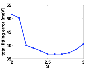
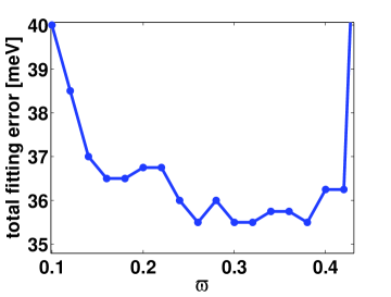
(a) Total fitting error as a function of $S$ and $\varpi$.

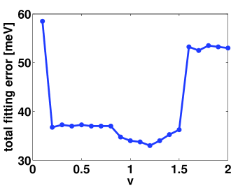
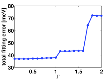
(b) Total fitting error as a function of $v$ and $\Gamma$.

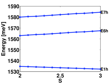
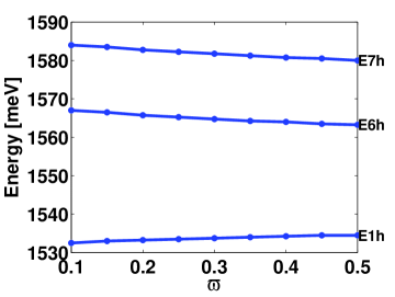
(c) The effect of the parameters $S$ and $\varpi$ on the position of the first three heavy hole exciton peaks.

Figure 2: The choice of the optimal calculation parameters.

In the next step we tried to fit the experimental line shapes (oscillator strengths). We have observed that variations of the coherence radius change substantially the lineshapes. The best fit was obtained for $\rho_{0L}=0.17\leavevmode\nobreak\ a^{*}_{L},\rho_{0H}=0.1\leavevmode\nobreak\ a^{*}_{H}$. It can be also verified that the increase of the damping parameter $\mit\Gamma$ results the lowering of the oscillator strength.

6 Conclusions

We have developed a simple mathematical procedure to calculate the optical functions of wide parabolic quantum wells. Our procedure describes the optical properties of a QW, taking into account the Coulomb interaction between electrons and holes. Our treatment includes anisotropic properties of the QW, and takes into account coherence of the electron-hole pair with the radiation field. The presented method has been used to investigate the optical functions of GaAs/Ga_1-xAl_xAs parabolic Quantum Well for the case of radiation incidence parallel to the growth direction and it shows an excellent agreement with the experimental data, explaining the number and the positions of the absorption maxima. The justification of the choice of effective potential parameters and the damping constant is also presented.

References

[1]
R. C. Miller, A. C. Gossard, D. A.Kleinman, and O. Munteanu,
Phys. Rev. B 29, 3740 (1984).
[2]
E. G. Gwinn, R. M. Westervelt, P. F. Hopkins, A. J. Rimberg, M.
Sundaram, and A. C. Gossard, Phys. Rev. B 39, 6260
(1989).
[3]
L. Brey, N. F. Johnson, and B. I. Halperin, Phys. Rev. B
40, 10647 (1989).
[4]
K. Karraï, M. Stopa, X. Ying, H. D. Drew, S. Das Sarma, and M.
Shayegan, Phys. Rev. B 42, 9732 (1990).
[5]
A. Wixforth, M. Sundaram, K. Ensslin, J. H. English, and A. C.
Gossard, Phys. Rev. B 43, 10000 (1991).
[6]
M. Sundaram, S. J. Allen, Jr., M. R. Geller, P. F. Hopkins, K. L.
Campman, and A. C. Gossard, Appl. Phys. Lett. 65, 2226 (1994).
[7]
H. Sari, Y. Ergün, and I. Sökmen, Superlatt. and
Microstruct. 17, 187 (1995).
[9]
N. A. El-Meshad, H. M. Hassanain, and H. H. Hassan, Egypt. J. Sol.
24, 1 (2001).
[10]
A. Matos-Abiague, Semicond. Sci. Technol. 17, 150 (2002).
[11]
R. T. Senger and K. K. Bajaj, Phys. Stat. Sol. B 236, 82
(2003).
[12]
G. Czajkowski and Ł. Skowroński, Adv. Studies Theor. Phys.
1, 187 (2007).
[13]
A. Tabata, M. R. Martins, J. B. B. Oliveira, T. E. Lamas, C. A.
Duarte, E. C. F. da Silva, and G. M. Gusev, J. Appl. Phys. 102,
093715 (2007).
[14]
A. Tabata, J. B. B. Oliveira, E. C. F. da Silva, T. E. Lamas, C.
A. Duarte, and G. M. Gusev, J. Phys. Conf. Series. 210, 012052
(2010).
[15]
A. Taqi and J. Diouri, Semicon.Phys., Quantum Electronic and
Optoelectronics 15, 21 (2012).
[16]
J. L. Birman, Electrodynamics and Nonlocal Optical Effects
mediated by Excitonic Polaritons, in Excitons, Modern
Problems in Condensed Matter Sciences, edited by E. I. Rashba,
and M. G. Sturge, Vol.2 (North-Holland, Amsterdam, 1982), p. 27.
[17]
S. I. Pekar, Crystal Optics and Additional Light Waves
(Benjamin- Cummings, Menlo Park, 1983).
[18]
V. M. Agranovich and V. L. Ginzburg, Crystal Optics with
spatial Dispersion and Excitons (Springer Verlag, Berlin, 1984).
[19]
A. D’Andrea and R. Del Sole, Phys. Rev. B 32, 2337 (1985).
[20]
K. Cho, J. Phys. Soc. Japan 55, 4113 (1986).
[21]
A. Stahl and I. Balslev, Electrodynamics of the Semiconductor
Band Edge (Springer-Verlag, Berlin-Heidelberg-New York, 1987).
[22]
A. D’Andrea and R. Del Sole, Phys. Rev. B 38, 1197 (1988).
[23]
G. Czajkowski, F. Bassani, and A. Tredicucci,
Phys. Rev. B 54, 2035 (1996).
[24]
G. Czajkowski, F. Bassani, and L. Silvestri, Rivista del Nuovo
Cimento 26, 1-150 (2003).
[25]
V. M. Agranovich, Excitations in Organic Solids (Oxford
University Press, Oxford, 2009).
[26]
G. Czajkowski and L. Silvestri 2006. Central European Journ. of
Physics 4, 254 (2006).
[27]
M. Tadić, F. M. Peeters, Phys. Rev. B 79
153305-1-4 (2009).
[28]
P. Schillak, European Phys. Journ. B 84
17 (2011).
[29]
J. H. Davies, The Physics of Low-Dimensional
Semiconductors (University Press Cambridge, 1998).
[30]
M. Grundmann,O. Stier, and D. Bimberg, Phys. Rev. B 52,
11969 (1995).