Local reversibility and entanglement structure of many-body ground states.

Abstract

The low-temperature physics of quantum many-body systems is largely governed by the structure of their ground states. Minimizing the energy of local interactions, ground states often reflect strong properties of locality such as the area law for entanglement entropy and the exponential decay of correlations between spatially separated observables. Here, we present a novel characterization of quantum states, which we call ‘local reversibility’. It characterizes the type of operations that are needed to reverse the action of a general disturbance on the state. We prove that unique ground states of gapped local Hamiltonian are locally reversible. This way, we identify new universal features of many-body ground states, which cannot be derived from the aforementioned properties. We use local reversibility to distinguish between states enjoying microscopic and macroscopic quantum phenomena. To demonstrate the potential of our approach, we prove specific properties of ground states, which are relevant both to critical and non-critical theories.

I Introduction

Gapped ground states define quantum phases of matter at zero temperature. Even though they occupy a tiny fraction of the possible many-body Hilbert space, these states manifest a rich and diverse structure. Standard examples are states with local order-parameter such as paramagnetic and ferromagnetic ground states, the superfluid and insulator ones in bosonic and fermionic many-body systems, etc. Other instances, such as quantum Hall and quantum spin liquids, can arise because of more subtle orders that can be established in the system. A central goal of condensed matter theory is to understand their structure and how it relates to the physics of different phases Wen (2004); Chen et al. (2010). A natural approach to this problem is to find the constraints that these states satisfy, which set them apart from generic many-body states Hayden et al. (2006). Such analysis can serve for the understanding of which type of entanglement that ground states can indeed harbour. To this aim, it is important to understand aspects of locality in these states. We ask: ‘to what extent can such states be described by a collection of local degrees of freedom, which are only loosely correlated with each other?’

Rigorous tools to tackle this question are scarce, even though various properties have been known in empirical ways (see Osborne (2012)). An example is provided by the exponential decay of correlations, also known as exponential clustering: it has been proved that gapped ground states on a lattice have a finite correlation length, beyond which the correlations between spatially separated observables decay exponentially Hastings (2004); Hastings and Koma (2006); Nachtergaele and Sims (2006). More recently, other quantitative tools have been devised, which characterize the ground state’s locality by looking at its entanglement structure Eisert et al. (2010); Amico et al. (2008). A notable example is area law of the entanglement entropy Eisert et al. (2010), which states that the entanglement entropy of a region with respect to the rest of the lattice should scale like the boundary area of the region rather than its volume. It is expected to hold for all gapped ground states on a lattice, but has only been rigorously proved in one spatial dimension (1D) by Hastings Hastings (2007a) (see Refs. Arad et al. (2012, 2013); Cho (2014); Brandão and Horodecki (2013); Arad et al. (2016a) for further results). Hastings’ celebrated result yields a complete characterization of 1D gapped ground states as matrix product states (MPS) Verstraete et al. (2008), which, to a large extent, provides a full understanding of the 1D case Chen et al. (2011).

Unfortunately, in higher spatial dimensions our understanding of the problem is still very much limited. Not only that a proof for the area law is lacking, but it is also unclear how an area law would imply an efficient representation of the ground state Ge and Eisert (2016). Moreover, when the system has long-range interactions, or it is hosted in a lattice with a large dimensionality (like an expander graph Hoory et al. (2006)), locality properties of the ground state are even more illusive: exponential decay of correlations no longer holds (since all particles are essentially close to each other), and in general, area law become meaningless as surface areas become as large as volumes. For such systems, very well studied in the Hamiltonian complexity field, spatial distance might no longer a good figure of merit for identifying entanglement Kempe et al. (2006); Hastings (2007b); Aharonov et al. (2013). As we will shortly show, an alternative approach is to study entanglement and locality by analyzing the collective properties of a subsystem with respect to the number of local degrees of freedom it contains rather than the distance between them.

In this paper, we introduce a new constraint on a many-body gapped ground states which complements some of the shortcomings of the existing approaches. We call it local reversibility. It is based on the intuition that macroscopic-scale entanglement cannot be recovered by any local operation once it has been broken. Therefore, states which allow this sort of local recovery, necessarily contain a ’small amount of macroscopic superposition’. Here, we observe that we use the term locality in a broader meaning than the usual spatial locality.

We will show that such local reversibility holds for all unique gapped ground states of local Hamiltonians, including systems with long-range interactions or a diverging lattice dimensionality (for which the existing approaches to the locality properties, like the exponential decay of correlation, do not apply). We therefore believe that it exposes fundamental features of gapped ground states that cannot be captured by existing properties. To demonstrate its potential, we study specific problems in many-body physics. We work out rigorous bounds for the quantum fluctuations of locally reversible states. This, in turn, implies new constraints on the critical exponents and rigorous bounds on the quality of the mean-field ansatz, which is often used to treat complicated quantum many-body systems. An important outcome of our approach is an effective way to identify quantum macroscopic superposition.

II Local reversibility

To motivate our approach, we begin with a heuristic discussion (Fig. 1). Consider a state $|\psi\rangle$ that is defined over $N$ localized spins, each with a $d$-dimensional Hilbert space, and let $\Gamma_{L}$ be an operator acting on a spin subset $L$; the total system is given by $L\cup L^{\rm c}$ with $L^{\rm c}$ the complement of $L$. Applying $\Gamma_{L}$ to $|\psi\rangle$, we can potentially disrupt the entanglement between $L$ and $L^{\rm c}$, even when $\Gamma_{L}|\psi\rangle$ has a constant overlap with $|\psi\rangle$. It is useful to think of $|\psi\rangle$ as a superposition of several states $|\psi\rangle=|\psi_{1}\rangle+|\psi_{2}\rangle+\cdots$ and of $\Gamma_{L}$ as a projector that “kills” some (but not all) of these states. Intuitively, if $|\psi\rangle$ contains some “global entanglement” on the scale of $|L|$ spins, we may only be able to reconstruct $|\psi\rangle$ by acting on $\Gamma_{L}|\psi\rangle$ with (at least) an operator that acts non-trivially on the same portion $L$ of the system (i.e., it would be an $|L|$-local operator). However, when $|\psi\rangle$ contains mostly short-range entanglement, we might be able to return to $|\psi\rangle$ by using an operator of a much smaller support. How much smaller should that support be for a slightly entangled state? Specifically, as we shall see shortly, the minimal size of support that is needed to reconstruct a product state is $\mathcal{O}(\sqrt{|L|})$. This indicates that states that can be reversed by operators of $\mathcal{O}(\sqrt{|L|})$ support constitute a class of states with a small amount of entanglement. In the following, we refer to such a class as locally reversible states.

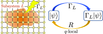
Figure 1: Schematic picture of the local reversibility (LR). We disturb a quantum state $|\psi\rangle$ by an operator $\Gamma_{L}$, which is supported in a subsystem $L$. We then try to recover the state $\Gamma_{L}|\psi\rangle$ by the use of a $q$-local operator $R$. If the state $|\psi\rangle$ is a product state, we can recover the original state by an operator $R$ with $q=\mathcal{O}(\sqrt{|L|})$; then, ‘locally reversible state’ is defined as the class of states which have the same property as product state in terms of the non-locality of the reverse operator. The entanglement properties of LR states are expected to be highly restricted since entanglement cannot be recovered by local operations once it has been broken.

We now put the discussion above on a formal ground. We first defines the notion of $q$-local operator, which may be often called a “few-body operator:”

Definition II.1 (${\bm{q}}$-local)

Given an integer $q>0$, a $q$-local operator is an operator of the form $O:=\sum_{|X|\leq q}o_{X}$, where each $o_{X}$ is an operator supported on a finite subset of spins $X=\{i_{1},i_{2},\ldots,i_{|X|}\}$ of cardinality $|X|$. The $o_{X}$ operators are not necessarily sitting next to each other on the lattice.

We formulate the reversibility property in terms of such operators $o_{X}$.

Definition II.2 (Local Reversibility)

We say that a state $|\psi\rangle$ is locally reversible (LR) if there exists a function $f(x)$ that decays faster than any power law, such that for every subset of spins $L$ and an operator $\Gamma_{L}$ defined on it, and for every integer $q>0$, there exists a $q$-local operator $R$ such that

$$\|R\Gamma_{L}|\psi\rangle-|\psi\rangle\|\leq\frac{\|\Gamma_{L}\|}{|\langle\psi|\Gamma_{L}|\psi\rangle|}f\biggl{(}\frac{q}{\sqrt{|{L}|}}\biggr{)}\,,$$ (1)

where $\|\cdots\|$ is the operator norm.

Three remarks are in order. i) Both the shape and the size of $L$ are left completely general. In particular, we can take $L$ to be the entire system ($|L|=N$). ii) In some cases, it will make sense to only consider operators $R$ that respect certain symmetries. We will later use this restricted definition of local reversibility for states with symmetry protected topological order (SPTO) Chen et al. (2013). The last remark is on the status of function $f(x)$ in (1). Despite $f(x)$ need to be a superpolynomially decaying function in II.2, the statement (1) itself can be proved for a fixed generic $f(x)$. In this sense, the statement is non-asymptotic and valid for finite systems. In order (1) to be effective in putting bounds on the state in a meaningful way, however, $f(x)$ need to be specific and non-trivial (see our main theorem III.1 for an example of $f(x)$); such a feature will be thoroughly exploited in the rest of the paper.

We claim that LR states show a specific degree of locality, while non-LR states correspond to states with non-local features due to global entanglement. This assertion can be explained by the following two lemmas characterizing the entanglement structure of LR states.

The first lemma refers to the so-called macroscopicity of the states. Namely, we will demonstrate how non-LR states correspond to states with macroscopic superposition.

Let’s consider states of the type $|\psi\rangle=\alpha|\psi_{a}\rangle+\beta|\psi_{b}\rangle$ and discuss the possibility that $|\psi_{a}\rangle$ and $|\psi_{b}\rangle$ are macroscopically distinct (meaning that a collection of local operators exists to $|\psi_{a}\rangle\leftrightarrow|\psi_{b}\rangle$). Then:

Lemma II.3

Let $|\psi\rangle$ be a state which satisfies (1) for a fixed function $f(x)$. Then, for any decomposition $|\psi\rangle=P_{L}|\psi\rangle+({\mathbb{I}}-P_{L})|\psi\rangle:=\alpha|\psi_{a}\rangle+\beta|\psi_{b}\rangle$ with $P_{L}^{2}=P_{L}$, we have

$$O|\psi_{a}\rangle=|\psi_{b}\rangle+|\delta\rangle,$$

where $O$ is a $q$-local operator and ${\|\delta\|^{2}}:=\langle\delta|\delta\rangle\leq|\alpha^{2}\beta|^{-1}f(q/\sqrt{|L|})$. When $|\psi\rangle$ is a LR state, $f(x)$ decays superpolynomially and only a difference of $\mathcal{O}(\sqrt{|L|})$ exists between the two states $|\psi_{a}\rangle$ and $|\psi_{b}\rangle$.

The proof is provided in the Appendix A.

By contraposition of the lemma, any quantum state such that we can find a bipartition $P_{L}$ for which two states $|\psi_{a}\rangle$ and $|\psi_{b}\rangle$ are macroscopically distinct over a $\sqrt{|L|}$ spatial scale, is non-LR; for example, the GHZ state over $n$ particles, $|\psi\rangle=\frac{1}{\sqrt{2}}(|0\cdots 0\rangle_{n}+|1\cdots 1\rangle_{n})$ is not LR since $|0\cdots 0\rangle_{n},|1\cdots 1\rangle_{n}$ are clearly macroscopically distinct over the scale of $n-1$, and we may write $|\psi\rangle=P_{L}|\psi\rangle+({\mathbb{I}}-P_{L})|\psi\rangle$ with $P_{L}:=|0\cdots 0\rangle\langle 0\cdots 0|_{n}$. As we show later, this simple lemma also shows that degenerate topologically ordered states are not LR.

The second lemma shows that fluctuations in an LR state are strongly suppressed. Indeed, consider an LR state $|\psi\rangle$ together with a subset of spins $L$, and let $A_{L}$ be an additive operator of the form $A_{L}:=\sum_{i\in L}a_{i}$. Here, each $a_{i}$ is an Hermitian operator with $\|a_{i}\|\leq 1$, which acts only on the $i$th spin. Since the $a_{i}$ operators are commuting with each other, they can be viewed as classical random variables whose joint probability distribution is given by the underlying state $|\psi\rangle$. The following lemma shows that their sum resembles a sum of independent random variables: its probability distribution is strongly concentrated around its mean with a width of $\mathcal{O}(\sqrt{|L|})$.

Lemma II.4

Let $\Pi^{A}_{\leq x}$ and $\Pi^{A}_{>x}$ be the projectors onto the eigenspaces of $A_{L}$ with eigenvalues $\leq x$ and $>x$ respectively, and let $m$ be the median of $A_{L}$ with respect to $|\psi\rangle$ satisfying (1) in the sense that $\langle\psi|\Pi^{A}_{\leq m}|\psi\rangle\geq 1/2$ and $\langle\psi|\Pi^{A}_{\geq m}|\psi\rangle\geq 1/2$. Then, for any positive $h$ the following inequality holds:

$$\|\Pi^{A}_{\geq m+h}|\psi\rangle\|\leq 2f\biggl{(}\frac{\lceil h/2\rceil-1}{\sqrt{|L|}}\biggr{)}\,.$$ (2)

with a fixed function $f(x)$. An equivalent statement is valid for $\|\Pi^{A}_{\leq m-h}|\psi\rangle\|$.

The proof is given by choosing $P_{L}=\Pi^{A}_{\leq m}$ in Lemma II.3. After a short algebra, we get $\|\Pi^{A}_{\geq m+h}|\psi\rangle\|\leq|\beta|\cdot\|\Pi^{A}_{\geq m+h}O\Pi^{A}_{\leq m}\|+2f(q/\sqrt{|L|})$ with $O$ $q$-local, where we use the facts $|\alpha|^{2}=\langle\psi|\Pi^{A}_{\leq m}|\psi\rangle\geq 1/2$ and $\|\Pi^{A}_{\geq m+h}|\psi_{b}\rangle\|=\|\Pi^{A}_{\geq m+h}|\psi\rangle\|/\beta$. To finish the proof we will show that $\|\Pi^{A}_{\geq m+h}O\Pi^{A}_{\leq m}\|=0$ for $q<h/2$. This follows from the fact that $A_{L}$ is a sum of (commuting) 1-local operators of norm 1, and therefore every $q$-local operator can take an eigenvector $|a\rangle$ of $A_{L}$ with eigenvalue $a$ to a superposition of eigenvectors $\sum c_{a^{\prime}}|a^{\prime}\rangle$ with $|a^{\prime}-a|\leq 2q$. Thus, choosing $q=\lceil h/2\rceil-1$ proves the lemma.

An immediate consequence of Lemma II.4 with the assumption that $f(x)$ is a super polynomially decaying function, is that the fluctuations of every additive operator $A_{L}$, which is defined on the entire systems ($|L|=N$) must satisfy

$$\langle(\Delta A_{L})^{2}\rangle:=\langle\psi|A_{L}^{2}|\psi\rangle-\langle\psi|A_{L}|\psi\rangle^{2}\leq\mathcal{O}(N)\,.$$ (3)

We point out that the well-known notion of macroscopicity measured by the Fisher information Shimizu and Morimae (2005); Fröwis and Dür (2012) is implied by the Lemma II.3 and Lemma II.4. This feature emerges clearly from the following reasoning. The Fisher information of a pure state $|\psi\rangle$ with respect to an operator $A$ is given by $\mathcal{F}(\psi,A)=4\langle(\Delta A)^{2}\rangle$ Fröwis and Dür (2012). In LABEL:frowis2012 the authors suggest to define the ‘effective macroscopic size’ of a state as $N_{\text{eff}}(\psi):=\max_{A}\mathcal{F}(\psi,A)/(4N)$, where the maximization is over all extensive operators $A:=\sum_{i}a_{i}$ as in (3). States showing maximal quantum macroscopicity, such as the GHZ state, have $N_{\text{eff}}=\mathcal{O}(N)$, whereas states with no quantum macroscopicity have $N_{\text{eff}}=\mathcal{O}(1)$. Inequality (3) therefore implies that LR states have $N_{\text{eff}}=\mathcal{O}(1)$. Equivalently, states with $N_{\text{eff}}=\mathcal{O}(N^{p})$ for $p>0$ are necessarily non-LR.

On the other hand, the converse is not true: there are states with $N_{\text{eff}}=\mathcal{O}(1)$ that are also non-LR. For instance, as we shall see, degenerate topologically ordered states turn out non-LR, but still satisfy the inequality (2), namely $N_{\text{eff}}=\mathcal{O}(1)$. Thereby, LR provides us a more stringent characterization of the macroscopic superposition encoded in a many-body state.

III Reversibility of ground states

We now introduce our main tool for identifying LR states. The following theorem states that unique gapped ground states of local Hamiltonians are LR. It holds for a very wide class of quantum systems that are described by $k$-local Hamiltonians of the form

$$H=\sum_{|X|\leq k}h_{X}\quad{\rm with}\sum_{X:X\ni{i}}\|h_{X}\|\leq g\quad\forall i\,,$$ (4)

where $g$ is a constant of $\mathcal{O}(1)$. Note that $k$ is not necessarily equal to $q$ from the definition of the operator $R$ above. Also note that we implicitly assume that the spins sit on a lattice, but we make no direct use of the lattice structure or its dimensionality. Instead, we use the second condition in (4), meaning that the total strength of all interactions in which the $i$th spin participates is bounded by a constant of $\mathcal{O}(1)$. This definition of $H$ captures a very wide class of quantum systems: with short-range interactions such as the the $XY$ model, the Heisenberg model Haldane (1983) and the AKLT model Affleck et al. (1987), as well as models with long-range interactions such as the Lipkin-Meshcov-Glick model Lipkin et al. (1965). Typically, we have $k=2$ (i.e., two-body interaction), but several exceptions exist such as the 1D cluster-Ising model Cui et al. (2013) ($k=3$), the toric code model on a square lattice Kitaev (2003) ($k=4$) and the string-net model on a honeycomb lattice Levin and Wen (2005) ($k=12$). We denote the ground state of $H$ by $|\Omega\rangle$, and fix its energy to be $E_{0}=0$. The rest of the energies are denoted by $0=E_{0}<E_{1}\leq E_{2}\leq\cdots$. Finally, we let $\delta E:=E_{1}-E_{0}$ be the spectral gap just above the ground state. With this notation at hand, our main theorem is given as follows.

Theorem III.1

With the above notations, for every spin subset $L$ and every operator $\Gamma_{L}$ defined on it, and for any positive integer $q$, there exists a $q$-local operator $R$ that satisfies

$$\|R\Gamma_{L}|\Omega\rangle-|\Omega\rangle\|\leq\frac{6\|\Gamma_{L}\|}{|\langle\Omega|\Gamma_{L}|\Omega\rangle|}e^{-2n_{0}/\xi},$$ (5)

where $n_{0}:=\lfloor q/k\rfloor$ and

$$\xi:=\sqrt{1+\frac{2E_{c}}{\delta E}},\quad E_{c}={g|L|}+8gkn_{0}.$$ (6)

Inequality (5), together with the definitions of $n_{0}$ and $\xi$, implies that $\|R\Gamma_{L}|\Omega\rangle-|\Omega\rangle\|\leq\frac{6\|\Gamma_{L}\|}{|\langle\Omega|\Gamma_{L}|\Omega\rangle|}e^{-\mathcal{O}(q\sqrt{\delta E/|L|})}$, and therefore $|\Omega\rangle$ is LR when $\delta E=\mathcal{O}(1)$. Hence the existence of a spectral gap places strong restrictions on structure of the ground states for very wide class of Hamiltonians. We note that the theorem requires no assumption on a spectral gap or the size of $|L|$ and $N$; hence, the theorem is not asymptotic and applicable for arbitrary ground states in finite systems.

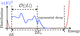
Figure 2: Schematic picture of the proof. After applying the operator $\Gamma_{L}$ to the ground state $|\Omega\rangle$, the energies at most of order $\mathcal{O}(|L|)$ are excited (blue curve). We then filter out the excited states by an approximate boxcar function in the range $[\delta E,2E_{c}+\delta E]$ (red curve). Although the function rapidly increases for $x\geq 2E_{c}+\delta E$, this can be cancelled by the exponential decay of the energy excitation.

The full proof of Theorem III.1 is given in Appendix B. Here we summarize its main ideas. Using recent results from LABEL:ref:Arad14-Edist, we conclude that after applying the operator $\Gamma_{L}$ to the ground state $|\Omega\rangle$, we get a state which consists mainly of excitations with energies of at most $\mathcal{O}(|L|)$. Beyond that scale, the weight of the excitations decays exponentially. This is shown schematically by the blue curve in Fig. 2. Then following ideas from a recent new proof of the 1D area law Arad et al. (2013), we construct the operator $R$ by approximating the ground-state projector using a polynomial of $H$. This polynomial is essentially a scaled version of the Chebyshev polynomial (red curve in Fig. 2), chosen such that it approximately behaves as a boxcar function in the range $[\delta E,2E_{c}+\delta E]$, thereby suppressing the majority of excitations in $\Gamma_{L}|\Omega\rangle$. Crucially, even though it rapidly increases for $x\geq 2E_{c}+\delta E$, this blowup is cancelled by the exponential decay of the high-energy excitation.

IV Examples of locally vs. non-locally reversible states

Let us now apply Lemmas II.3, II.4 and Theorem III.1 to several exemplary states emerging in different contexts. The list of states is summarized in Table 1. In particular, we will demonstrate how local reversibility implies the absence of macroscopic superposition. We begin with LR states.

1. Product states. A product state $|\psi\rangle=|\psi_{1}\rangle\otimes|\psi_{2}\rangle\otimes\cdots\otimes|\psi_{N}\rangle$ is LR because it is the unique ground state of the local Hamiltonian $H=\sum_{i=1}^{N}({\mathbb{I}}-|\psi_{i}\rangle\langle\psi_{i}|\otimes{\mathbb{I}}_{\rm rest})$. As $H$ is made of commuting projectors, its spectral gap is necessarily $\delta E=1$.

2. Graph states with bounded degree. These states are defined on a graph in which each node has at most $\mathcal{O}(1)$ neighboring nodes Raussendorf and Briegel (2001); Briegel and Raussendorf (2001) . The graph state is a non-degenerate gapped ground states of a Hamiltonian which is the summation of the following commuting stabilizers Hein et al. (2004) $\{g_{i}\}_{i=1}^{N}$: ${g_{i}=\sigma_{i}^{x}\otimes(\sigma_{j_{1}}^{z}\sigma_{j_{2}}^{z}\cdots\sigma_{j_{k_{i}}}^{z}),}$ where $[g_{i},g_{i^{\prime}}]=0$ for $\forall i,i^{\prime}$, $\{\sigma^{x},\sigma^{y},\sigma^{z}\}$ are the Pauli matrices and $\{j_{1},j_{2},\ldots,j_{k_{i}}\}$ are nodes which connect to the node $i$. By assumption, $k_{i}=\mathcal{O}(1)$, and hence the Hamiltonian is $\mathcal{O}(1)$-local. By the commutativity of its terms, we conclude that it has a spectral gap $\delta E=\mathcal{O}(1)$, and so by Theorem III.1 such graph states are LR.

3. Short-range entanglement (SRE) states. The third example are states that can be obtained by a constant-depth quantum circuit acting on a product state. In the literature they are often dubbed as “trivial states” Hastings (2011); Freedman and Hastings (2014), or “short-range-entanglement (SRE) states” Chen et al. (2010). A constant-depth quantum circuit is a unitary operator that can be written as a product of $k=\mathcal{O}(1)$ unitary operators $U=U_{1}\cdots U_{k}$ where each unitary $U_{i}$ is given as a product of unitary operators $U_{i}=U_{i,1}\cdot U_{i,2}\cdots U_{i,n_{i}}$ with non-overlapping support of $\mathcal{O}(1)$. To see why these are LR states, we write $|\psi\rangle=U|\phi\rangle$, where $U$ is the constant-depth circuit, and $|\phi\rangle=|\phi_{1}\rangle\otimes|\phi_{2}\rangle\otimes\cdots$ is a product state. Then it is easy to see that for any operator $O$ with a support of $\mathcal{O}(1)$, $UOU^{-1}$ has also an $\mathcal{O}(1)$ support, and therefore if $H$ is a local Hamiltonian for which $|\phi\rangle$ is the unique ground state (see the first example), then $H^{\prime}=UHU^{-1}$ is also a local Hamiltonian. Furthermore, $H^{\prime}$ has the same spectrum as $H$, and so it is gapped with the unique ground state, which is exactly $|\psi\rangle$. By Theorem III.1 this state is LR.

We note that not all LR states are also SRE states, or, equivalently, long-range entanglement (LRE) does not necessarily imply non-LR. For example, Kitaev’s toric code Kitaev (2003) on a sphere is a commuting local Hamiltonian and has a non-degenerate ground state with an $\mathcal{O}(1)$ gap, and therefore by Theorem III.1 it is LR. Nevertheless, it cannot be generated by a constant depth circuit working on a product state, and is therefore not an SRE state Hastings (2012). This point is also explained in Appendix C.

Table 1: Locally Vs non-locally reversible states
LR	Non-LR
Product state	GHZ state
Bounded-degree graph states	States with large fluctuation
Short-range entangled state	Degenerate, topologically ordered ground states
	Degenerate, SPTO states (Symmetry-restricted non-LR)

We now turn to non-LR states. We will use Lemmas II.3 and II.4 to identify such states.

5. “Schrödinger Cat” like states. States like the GHZ are not LR by Lemma II.3.

6. States with Fisher information of $\mathcal{O}(N^{p})$ with $p>1$. As we already mentioned, this result comes directly from Lemma II.4. Also here, a quintessential example of this class is the GHZ state Fröwis and Dür (2012), which has the scaling with $p=2$. Moreover, the ground states at critical point are typically non-LR since they have $p=1+(2-\eta-z)/D$ (see Appendix E), where $z$ is the dynamical critical exponent, $\eta$ is the anomalous critical exponent, and $D$ is the dimension of the system. For example, the critical point of the 1D transverse Ising model has $z=1$ and $\eta=1/4$, which yields $p=7/4$.

7. States with degenerate topological order. While the local fluctuations in Lemma II.4 (as well as the Fisher information) cannot detect a locally hidden order such as the topological order, we can use Lemma II.3 to see that states with a degenerate topological order are not LR. We demonstrate this point using Kitaev’s toric code model on a torus Kitaev (2003) with $\sqrt{n}\times\sqrt{n}$ sites. The idea is that by taking $L$ to be a non-trivial loop in the torus of size $\sqrt{n}$, there exists an operator $T_{L}$ that takes one ground state $|\Omega_{1}\rangle$ to another ground state $|\Omega_{2}\rangle$, i.e., $|\Omega_{2}\rangle=T_{L}|\Omega_{1}\rangle$. The properties of the topological order guarantee that for any observable $O$ that is supported on less than $\sqrt{n}$ sites (the size of a Wilson loop), $\langle\Omega_{1}|O|\Omega_{1}\rangle=\langle\Omega_{2}|O|\Omega_{2}\rangle$ and $\langle\Omega_{1}|O|\Omega_{2}\rangle=0$. Therefore, we may invoke Lemma II.3 with $P_{L}:=({\mathbb{I}}-T_{L})/2$, such that $|\Omega_{1}\rangle=P_{L}|\Omega_{1}\rangle+({\mathbb{I}}-P_{L})|\Omega_{1}\rangle:=\alpha|\Omega_{+}\rangle+\beta|\Omega_{-}\rangle$, where $|\Omega_{\pm}\rangle=\frac{1}{\sqrt{2}}(|\Omega_{1}\rangle\pm|\Omega_{2}\rangle)$. It is easy to verify from the above properties that $|\Omega_{+}\rangle,|\Omega_{-}\rangle$ are macroscopically distinct over a scale of $\mathcal{O}(n^{1/4})$ (they are in fact distinct over a scale of $\sqrt{n}$, i.e., the size of $L$), and therefore by Lemma II.3, these degenerate ground states are not LR.

We remark that non-degenerate topological order (e.g., in the toric code on the surface) results LR (from Theorem III.1). In this context, we observe that, despite the topological entropy is non vanishing for both degenerate and non degenerate topologically ordered ground states, the two cases are clearly distinct in terms of the irreducible multiparty correlation (the issue has been recently addressed in Refs Zhou (2008); Kato et al. (2016); Liu et al. (2016); see also Appendix C): Being our approach able to detect a ‘fine structure’ in the nature of the multipartite correlations, LR tells degenerate topological order apart from non-degenerate topological order.

8. States with a degenerate symmetry protected topological order. The same arguments showing that degenerate topologically ordered states are not LR can be applied to the case of degenerate symmetry protected topological order. Such states show topological order only to a restricted set of operators defining a certain symmetry $G$ Chen et al. (2013). They cannot be adiabatically connected to a product state using only operators from $G$, and in that restricted sense they are not SRE (see the following for the definition). An important example of states with SPTO can be obtained from graph state’s Hamiltonian on an open lattice, where one removes the boundary stabilizers. This removal introduces degeneracy to the groundspace. Much like the case of Kitaev’s toric code, we can also show here that the resulting ground states are non-LR as long as we restrict the operator $R$ to satisfy the symmetry of the graph Hamiltonian without the boundary stabilizers. We refer to these states as symmetry restricted non-LR states. We present an example of such states for 1D case Son et al. (2012) in the Appendix D.

V Fluctuations in locally reversible states

Theorem III.1, together with Lemma II.4 provides a remarkable insight into the structure of unique ground states. For any such ground state $|\Omega\rangle$, and for any additive operator $A_{L}=\sum_{i\in L}a_{i}$ defined on a spin subset $L$, $\|\Pi^{A}_{\geq m+h}|\Omega\rangle\|\leq e^{-c_{1}h\sqrt{\delta E/|L|}}\,,$ with $c_{1}$ a constant of $\mathcal{O}(1)$ (with $m$ as defined in Lemma II.4). This implies that $|\langle A_{L}\rangle-m|=\mathcal{O}(|L|/\delta E)$, where $\langle A_{L}\rangle=\langle\Omega|A_{L}|\Omega\rangle$ is the expectation of $A_{L}$ in the ground state, and therefore

$$\|\Pi^{A}_{\geq\langle A_{L}\rangle+h}|\Omega\rangle\|\leq e^{-c_{2}h\sqrt{\delta E/|L|}}\,,$$ (7)

$c_{2}$ being a constant depending on the Hamiltonian’s parameters $k$ and $g$. Taking $A_{L}$ to be an order parameter (i.e., the magnetization in $L$), we arrive at the conclusion that the deviations of any order parameter from its expectation are exponentially suppressed in unique gapped ground states. It is interesting to contrast this inequality with the corresponding statistics of a product state. In such a case, $A_{L}$ can be viewed as a sum of independent random variables, and by the Hoeffding’s inequality  Hoeffding (1963), $\|\Pi^{A}_{\geq\langle A_{L}\rangle+h}|\psi\rangle\|\leq e^{-\mathcal{O}(h^{2}/|L|)}$. In this sense, unique gapped ground states enjoy a weaker, yet still non-trivial, notion of local independence.

It is also worth noting that this independence cannot be (at least directly) deduced from the exponential decay of correlation of gapped ground states Hastings and Koma (2006); Nachtergaele and Sims (2006), since it can be applied to sets of observables that may sit very close to each other on the lattice. Moreover, we can apply it to systems with long-range interactions, such as the Lipkin-Meshcov-Glick model Lipkin et al. (1965) and systems defined on the expander graphs Hoory et al. (2006), in which the maximal distance between any two spins is $\mathcal{O}(1)$ and $\mathcal{O}(\log N)$, respectively. We remark that inequality (7) can be extended to generic few-body operators Kuwahara (2016): $A=\sum_{|X|\leq q}a_{X}$ with $q=\mathcal{O}(1)$; finally we can derive a similar bound for low-lying energy states, i.e., not necessarily the exact ground state (T.K., I.A., L.A. and V. V., manuscript in preparation).

A simple consequence of inequality (7) is a trade-off relationship between the spectral gap and the fluctuation $\Delta A_{L}:=(\langle\Omega|A_{L}^{2}|\Omega\rangle-\langle\Omega|A_{L}|\Omega\rangle^{2})^{1/2}$ of $A$ in the ground state:

$$\delta E\cdot(\Delta A_{L})^{2}\leq{\rm const}\cdot|L|,.$$ (8)

This has two interesting implications:

1. Bounds on the critical exponents. As noted above, Theorem III.1 does not assume the spectral gap of $\mathcal{O}(1)$ and therefore can be applied to arbitrary ground states. Below, we apply it to quantum critical points to obtain a general inequality for critical exponents.

Let us consider the critical regime, $\delta E\to 0$. Define $A_{L}=\sum_{i=1}^{N}a_{i}$ with $L$ a total system and $\{a_{i}\}_{i=1}^{N}$ order parameters (e.g. magnetization). We then introduce the critical exponents $z$, $\eta$, $\gamma$ and $\nu$ as in Refs. Continentino (1994); $z$ is the dynamical critical exponent, $\eta$ is the anomalous critical exponent, $\gamma$ is the susceptibility critical exponent and $\nu$ is the correlation length exponent. By applying the finite-scaling ansatz Continentino (1994) to (8), we can obtain

$$z\geq 1-\frac{\eta}{2}=\frac{\gamma}{2\nu},$$ (9)

where the second equality comes from the Fisher equality $2-\eta=\gamma/\nu$. We remark that (9) holds for very general settings both for homogeneous and disordered critical systems (see Vojta and Schmalian (2005) for a non-trivial example where our inequality can be applied). Incidentally, we note that (8) gives non-trivial bounds for the critical Lipkin-Meshcov-Glick model, a system with long-range interactions Lipkin et al. (1965); Dusuel and Vidal (2004). The details of this calculation are given in Appendix E

2. Validity of mean-field approximations. Under the assumption of inequality (8) for ground states, we can estimate the validity of the mean-field approximation. Just as the first implication, the full details are given in Appendix F. The idea is that since the operators $A_{L}$ in (8) are arbitrary (as long as they are additive on $L$), we can use them to probe the two-spin reduced density matrix $\rho_{ij}$ and its relation with its mean-field approximation $\rho_{i}\otimes\rho_{j}$. Specifically, it can be shown that for every spin subset $L$ and an arbitrary spin $i$ outside of it,

$$\sum_{j\in L}\|\rho_{ij}-\rho_{i}\otimes\rho_{j}\|\leq{\rm const}\cdot\sqrt{|L|/\delta E}\,.$$ (10)

This implies that on average, for each spin $j\in L$, $\|\rho_{ij}-\rho_{i}\otimes\rho_{j}\|\leq\mathcal{O}(1/\sqrt{|L|\delta E})$. If our system is defined by a nearest-neighbor two-body Hamiltonian on a regular grid with coordination number $Z$ (the number of neighbors of each spin), then taking $L$ to be the set of neighbors ($|L|=Z$), one immediately obtains a bound on the quality of the mean-field approximation for the energy density for $\forall i$:

$$\biggl{|}\frac{1}{Z}\sum_{<i,j>}\langle h_{ij}\rangle_{\rm MF}-\frac{1}{Z}\sum_{<i,j>}\langle h_{ij}\rangle_{\rm exact}\bigg{|}\leq{\rm const}\cdot\frac{1}{\sqrt{Z\delta E}}\,,$$

where the sum is taken over the spins adjacent to $i$. We therefore obtain a quantitative bound on how the error of the mean-field approximation decreases as the lattice dimension (on which the coordination number depends) goes to infinity. This result is consistent with the folklore knowledge in condensed-matter physics that the mean-field becomes exact in infinite dimension. Recently, similar results have been obtained in different manners by Brandão et al. Brandão and Harrow (2013) and Osterloh et al. Osterloh and Schützhold (2015) In Ref. Brandão and Harrow (2013), the setup is more general (i.e., the system is not assumed to be gapped) but the error estimation is weaker than ours, scaling as $\mathcal{O}(Z^{-1/3})$: In Ref. Osterloh and Schützhold (2015), the error estimation is as good as ours, $\mathcal{O}(Z^{-1/2})$, but under the additional assumptions of having a regular, isotropic, and bipartite lattice of $\frac{1}{2}$-spins.

VI Summary and open questions

In this work, we introduced a new notion of locality in quantum states, the local reversibility, which is defined in terms of the type of local operations that are needed to reverse the action of perturbations to the state.

We proved that all unique ground states of gapped local Hamiltonians are locally reversible (Theorem III.1), and, on the other hand, we showed how local reversibility implies a suppression of quantum fluctuations (Lemma II.4). Together, these two results provide new insights into the structure of unique ground states of gapped local-Hamiltonians: i) a low Fisher information, which is an indication for the lack of quantum macroscopicity in these states; ii) a novel inequality for the critical exponents in these systems; iii) a quantitative analysis of the mean-field approximation; and finally, iv) since an adiabatic (local unitary) evolution of product states is locally reversible, our result clearly implies that all the gapped quantum phases of matter, disordered or with local order parameter (Landau symmetry breaking quantum phases), are reversible. In contrast, degenerate topological phases or the symmetry protected topological phases, are not reversible. We note that LR can detect the difference between degenerate and non degenerate topological order. Indeed, it was discovered that, although both with non vanishing topological entropy they have very different irreducible multipartite correlation (see paragraph 8 of SectIV and the Appendix C). In this context, we observe that LR can be further restricted (with a similar logic we pursued in this article to deal with symmetry protected topological phases) to improve and refine the characterisation of the ground state. Such a strategy might lead to catch properties of the state originating from the geometry of its ambient space.

Our work provides an instrumental view for several research directions.

Based on the bounds on the fluctuations we found, we might argue that, fluctuations in gapped ground state obey a Gaussian statistics (as they do in non interacting theories). A recent proof of the Berry-Esseen theorem for the quantum case by Brandão et al. Brandão and Cramer (2015) hints that this might be the case. A natural approach to this would be to tighten our main theorem, replacing the exponential decay in the RHS of inequality (5) by a Gaussian.

Another intriguing direction to pursue is to incorporate LR, or one of its consequences, such as Lemma II.4 or inequality (8), – explicitly or implicitly – in the construction of tensor networks in higher dimension (e.g., Projected entangled pair state, or PEPS Verstraete et al. (2008)). By construction, these states satisfy the area-law, but we now know that they should also satisfy local reversibility. This will speed up the contraction of such tensor networks, which is the main bottleneck in the variational algorithms Lubasch et al. (2014a, b); Anshu et al. (2016); Schwarz et al. (2016). A goal of paramount importance in this context is to prove that PEPS are faithful representations of gapped ground states. A good place to start studying this question is in the 1D world. We know that MPS can describe both LR and non-LR states (i.e., GHZ). The natural problem is then to pinpoint what is needed for an MPS to describe an LR state.

Proving the area-law conjecture for gapped systems in 2D and beyond remains a challenge. It would be interesting to see if the additional structure of local reversibility of these states can assist in such proofs, or at least provide new insights regarding this important conjecture. As a specific route, we suggest to harness the LR in addition to the clustering, to improve the upper bound by Brandão and Horodecki Brandão and Horodecki (2013).

Finally, it would be interesting to understand if local reversibility could somehow be used to characterize unique gapped ground states. In other words, is local reversibility also a sufficient condition for unique gapped ground states? Strictly speaking, this is incorrect, as there are LR states which are not gapped ground states. For example, the state $|000\cdots 0\rangle+\epsilon(N)|111\cdots 1\rangle$ where $\epsilon(N)$ decays faster than any polynomial is trivially LR, but can never be a unique gapped ground state of $k$-local Hamiltonians as long as $k\leq N/2$ (see LABEL:ref:Facchi11-GHZ). Nevertheless, we may still ask if, in some sense, every LR state can be approximated by a unique gapped ground state. If this is not the case, it would be interesting to understand which are these LR states that cannot be even approximated by gapped ground states.

Generalising our approach to mixed states and devising experimental protocols to measure local reversibility are important future challenge.

Appendix A Proof of Lemma II.3

Assume that $|\psi\rangle$ satisfies inequality (1). Then for every integer $q>0$, there exists a $q$-local operator $R$ such that $RP_{L}|\psi\rangle=|\psi\rangle+|\delta^{\prime}\rangle$, where $\|\delta^{\prime}\|^{2}\leq\frac{\|P_{L}\|}{|\langle\psi|P_{L}|\psi\rangle|}f(q/\sqrt{|L|})\leq\frac{1}{|\alpha|^{2}}f(q/\sqrt{|L|})$. Therefore,

$$\beta|\psi_{b}\rangle ={\mathbb{I}}|\psi\rangle-P_{L}|\psi\rangle=(R-{\mathbb{I}})P_{L}|\psi\rangle-|\delta^{\prime}\rangle$$

$$=\alpha(R-{\mathbb{I}})|\psi_{a}\rangle-|\delta^{\prime}\rangle\,.$$

By denoting $O=\alpha(R-{\mathbb{I}})/\beta$ and $|\delta\rangle=-\beta^{-1}|\delta^{\prime}\rangle$, we have $|\psi_{b}\rangle=O|\psi_{a}\rangle+|\delta\rangle$, where $\|\delta\|^{2}=\|\delta^{\prime}\|^{2}/|\beta|\leq\frac{1}{|\alpha^{2}\beta|}f(q/\sqrt{|L|})$. This completes the proof of Lemma II.3.

Appendix B Proof of Theorem III.1

B.1 Outline

The proof of Theorem III.1 is rather technical, and therefore we first sketch it here, giving the full details in the following section.

Multiplying inequality (5) by $|\langle\Omega|\Gamma_{L}|\Omega\rangle|$, and writing for brevity $\tilde{R}:=\langle\Omega|\Gamma_{L}|\Omega\rangle R$, we obtain

$$\|(\tilde{R}-|\Omega\rangle\langle\Omega|)\cdot\Gamma_{L}|\Omega\rangle\|\leq 6\|\Gamma_{L}\|e^{-2n_{0}/\xi}\,.$$ (11)

So for the state to be LR, we need to find a $\tilde{R}$ whose action on $\Gamma_{L}|\Omega\rangle$ approximates the action of the ground state projector $|\Omega\rangle\langle\Omega|$ on it. In addition, in order to satisfy the premise of the theorem, it has to be a $q$-local operator. To this aim, we look for a low-degree polynomial $F_{R}(x)$ and write $\tilde{R}:=F_{R}(H)$. Specifically, choosing a polynomial of degree $n_{0}:=\lfloor q/k\rfloor$ guarantees that it will contain at most $q$-local terms, since, by definition, each term in $H$ is $k$-local.

To understand the restrictions on $F_{R}(x)$ that inequality (11) poses, it is convenient to work in the energy basis $\{|E\rangle\}$: expanding $\Gamma_{L}|\Omega\rangle=\sum_{E}c(E)|E\rangle$, we want i) $F_{R}(0)=1$ (recall that have set $E_{0}=0$), and ii) $\left(\sum_{E\geq\delta E}|c(E)\cdot F_{R}(E)|^{2}\right)^{1/2}\leq 6\|\Gamma_{L}\|e^{-2n_{0}/\xi}$. This is achieved using two ideas, which are demonstrated in Fig. 2.

The first idea is that the expansion of $\Gamma_{L}|\Omega\rangle$ is dominated by energies of at most $\mathcal{O}(|L|)$; beyond that scale, $c(E)$ is exponentially decaying. This is a direct corollary of Theorem 2.1 in LABEL:ref:Arad14-Edist, which for our case implies:

Corollary B.1 (from Theorem 2.1 in LABEL:ref:Arad14-Edist)

Let $\Pi^{H}_{\geq E}$ be the projector into the eigenspace of $H$ with energies greater than or equal to $E$. Then

$$\sum_{E^{\prime}\geq E}|c(E^{\prime})|^{2}=\|\Pi^{H}_{\geq E}\Gamma_{L}|\Omega\rangle\|^{2}\leq\|\Gamma_{L}\|^{2}e^{-(E-2g|L|)/4gk}\,.$$ (12)

In LABEL:ref:Arad14-Edist, this theorem was proved under the more restricted condition that every particle participates in at most $g$ interactions of norm 1, but this can be easily relaxed to the current condition, given in definition (4).

The bound in (12) implies that our polynomial should mainly “kill” the energy excitations of $\Gamma_{L}|\Omega\rangle$ in the range $[\delta E,\mathcal{O}(|L|)]$. Following LABEL:ref:Arad-AL13, we let $F_{R}(x)$ be the $n_{0}$th order Chebyshev polynomial Abramowitz and Stegun (1972), scaled such that $x:[-1,1]\mapsto[\delta E,2E_{c}+\delta E]$ and $F_{R}(0)=1$. As discussed in the following section, this polynomial fluctuates between $\pm e^{-2n_{0}/\xi}$ in the range $[\delta E,2E_{c}+\delta E]$, and then diverges like $\mathcal{O}((2x/E_{c})^{n_{0}})$. It is our choice of $E_{c}$ in Theorem III.1 which guarantees that this divergence is cancelled by the exponential decay of Corollary B.1. After a rather straightforward calculation, one can show that total contributions of the energy segments $[\delta E,2E_{c}+\delta E]$ and $[2E_{c}+\delta E,\infty)$ to $\|(\tilde{R}-|\Omega\rangle\langle\Omega|)\cdot\Gamma_{L}|\Omega\rangle\|$ is exponentially small.

B.2 Full proof

Following the proof’s sketch in the previous section of the main text of the paper, we start from inequality (12). Our goal is to find a polynomial $F_{R}(x)$ such that the action of the operator $\tilde{R}:=F_{R}(H)$ on the state $\Gamma_{L}|\Omega\rangle$ approximates the action of the ground state projector $|\Omega\rangle\langle\Omega|$ on it. As $H$ is a $k$-local operator, choosing $n_{0}:=\lfloor q/k\rfloor$ guarantees that $\tilde{R}$ is a $q$-local operator.

Working in the eigenbasis of $H$, we expand $\Gamma_{L}|\Omega\rangle=\sum_{E}c(E)|E\rangle$, and as $F_{R}(H)$ is diagonal in this basis,

$$[F_{R}(H)-|\Omega\rangle\langle\Omega|]\Gamma_{L}|\Omega\rangle =(F_{R}(0)-1)c(0)|\Omega\rangle+\sum_{E\geq\delta E}F_{R}(E)c(E)|E\rangle\,.$$

Therefore, for inequality $(12)$ to hold, it is sufficient that

$$F_{R}(0)=1$$ (13)

$$\left(\sum_{E>\delta E}|c(E)F_{R}(E)|^{2}\right)^{1/2}\leq 6\|\Gamma_{L}\|e^{-2n_{0}/\xi}\,.$$ (14)

As noted in the outline of the proof in the previous section, to prove these properties we use two ideas. The first is that the weight of the high energy excitations in $\Gamma_{L}|\Omega\rangle$ decays exponentially, as shown in Corollary B.1 of Section B.1. The second is to take $F_{R}(x)$ to be a scaled version of the $n_{0}$’th order Chebyshev polynomial. Let us start from the second idea. The $n$th order Chebyshev polynomial Abramowitz and Stegun (1972) of the first kind is given by

$$T_{n}(x):=\frac{(x+\sqrt{x^{2}-1})^{n}+(x-\sqrt{x^{2}-1})^{n}}{2}\,.$$ (15)

Equivalently, for $x\in[-1,1]$ it is given by $T_{n}(x)=\cos(n\arccos(x))$, and for $|x|>1$ by $T_{n}(x)=\cosh(n\operatorname{arccosh}(x))$. What makes the Chebyshev polynomial so useful to our purpose are the properties that are summarized in the following lemma, whose proof is given in Sec. B.2.1:

Lemma B.2

$$|T_{n}(x)| \leq 1\ , |x|\leq 1$$ for (16)

$$|T_{n}(x)| \leq\frac{1}{2}(2|x|)^{n}\ , |x|\geq 1$$ for (17)

$$|T_{n}(x)| \geq\frac{1}{2}\exp{\left(2n\sqrt{\frac{|x|-1}{|x|+1}}\right)}\ , |x|\geq 1$$ for (18)

Setting

$$\xi:=\sqrt{1+\frac{2E_{c}}{\delta E}},\quad\text{and}\quad E_{c}:=g|L|+8gkn_{0}\,,$$ (19)

we define $F_{R}(x)$ to be the polynomial

$$F_{R}(x):=\frac{T_{n_{0}}(\frac{x-\delta E}{E_{c}}-1)}{T_{n_{0}}(\frac{-\delta E}{E_{c}}-1)}\,.$$ (20)

In other words, we defined it to be the $n_{0}$th order Chebyshev polynomial, scaled such that $x:[-1,1]\mapsto[\delta E,2E_{c}+\delta E]$ and $F_{R}(0)=1$. Clearly, this definition satisfies Eq. (13). Let us see why it also satisfies inequality (14).

We begin by applying Lemma B.2 to the definition of $F_{R}(x)$, which implies that for $\delta E\leq x\leq 2E_{c}+\delta E$,

$$|F_{R}(x)|\leq 2e^{-2n_{0}/\xi}\,,$$ (21)

and for $x\geq 2E_{c}+\delta E$,

$$|F_{R}(x)| \leq\biggl{(}\frac{2x-2\delta E}{E_{c}}-2\biggr{)}^{n_{0}}e^{-2n_{0}/\xi}\,.$$ (22)

For brevity, we define the low and high energy ranges $I_{\rm LOW}:=[\delta E,2E_{c}+\delta E)$ and $I_{\rm HI}:=[2E_{c}+\delta E,\infty)$. Then using the triangle inequality, we split the sum in the LHS of (14)

$$\left(\sum_{E>\delta E}|c(E)F_{R}(E)|^{2}\right)^{1/2}\leq\left(\sum_{E\in I_{\rm LOW}}|c(E)F_{R}(E)|^{2}\right)^{1/2}+\left(\sum_{E\in I_{\rm HI}}|c(E)F_{R}(E)|^{2}\right)^{1/2}\,,$$

and bound each term separately. The low-energy term is bounded by

$$2e^{-2n_{0}/\xi}\left(\sum_{E\in I_{\rm LOW}}|c(E)|^{2}\right)^{1/2}\leq 2e^{-2n_{0}/\xi}\|\Gamma_{L}|\Omega\rangle\|\leq 2\|\Gamma_{L}\|e^{-2n_{0}/\xi}\,,$$ (23)

which follows from Inequality (21) and the fact that $\sum_{E\in I_{\rm LOW}}|c(E)|^{2}\leq\sum_{E}|c(E)|^{2}=\|\Gamma_{L}|\Omega\rangle\|^{2}$.

To finish the proof, we will show that the high energies term is upper bounded by $4\|\Gamma_{L}\|e^{-2n_{0}/\xi}$. To this aim, we write $I_{\rm HI}=I_{1}\cup I_{2}\cup I_{3}\cup\ldots$, where $I_{j}:=[2E_{c}+\delta E+(j-1)\eta,2E_{c}+\delta E+j\eta)$ and $\eta$ is a positive constant which will be set afterward. Using the triangle inequality once more, we get

$$\left(\sum_{E\in I_{\rm HI}}|c(E)F_{R}(E)|^{2}\right)^{1/2}\leq\sum_{j=1}^{\infty}\left(\sum_{E\in I_{j}}|c(E)F_{R}(E)|^{2}\right)^{1/2}\,.$$

Clearly, for each $I_{j}$ segment

$$\left(\sum_{E\in I_{j}}|c(E)F_{R}(E)|^{2}\right)^{1/2} \leq\max_{x\in I_{j}}|F_{R}(x)|\left(\sum_{E\in I_{j}}|c(E)|^{2}\right)^{1/2}\,.$$

As $|F_{R}(x)|$ monotonically increases for $x\geq 2E_{c}+\delta E$ (which follows from the fact that the Chebyshev polynomial is monotonic for $x\geq 1$), it follows that

$$\max_{x\in I_{j}}|F_{R}(x)|\leq|F_{R}(2E_{c}+\delta E+j\eta)|\,.$$

To bound the other term, we use Corollary B.1, which gives us

$$\left(\sum_{E\in I_{j}}|c(E)|^{2}\right)^{1/2}\leq\left(\sum_{E\geq 2E_{c}+\delta E+(j-1)\eta}|c(E)|^{2}\right)^{1/2}\leq\|\Gamma_{L}\|e^{-\lambda(2E_{c}+\delta E+(j-1)\eta-2g|L|))}\,,$$

where we have defined

$$\lambda:=\frac{1}{4gk}\,.$$ (24)

Together, this gives us

$$\left(\sum_{E\in I_{j}}|c(E)F_{R}(E)|^{2}\right)^{1/2}\leq\|\Gamma_{L}\|e^{\lambda\eta}\cdot\left|F_{R}(2E_{c}+\delta E+j\eta)\right|e^{-\lambda(2E_{c}+\delta E+j\eta-2g|L|)}\,.$$

The final step is to show that for $x\geq 2E_{c}+\delta E$,

$$|F_{R}(x)|\cdot e^{-\lambda(x-2g|L|)}\leq e^{-2n_{0}/\xi}\cdot e^{-\lambda(x-2g|L|)/2}$$ (25)

(see Subsection B.2.2 for a proof), which leads to

$$\left(\sum_{E\in I_{j}}|c(E)F_{R}(E)|^{2}\right)^{1/2}\leq\|\Gamma_{L}\|e^{-2n_{0}/\xi}e^{\lambda\eta}\cdot e^{-\lambda(2E_{c}+\delta E+j\eta-6g|L|)/2}\,.$$

Summing over all $j\geq 1$, then gives us

$$\left(\sum_{E\in I_{\rm HI}}|c(E)F_{R}(E)|^{2}\right)^{1/2}\leq\|\Gamma_{L}\|e^{-2n_{0}/\xi}\cdot e^{-\lambda(2E_{c}+\delta E-2g|L|)/2}\cdot e^{\lambda\eta}\sum_{j=1}^{\infty}e^{-j\eta\lambda/2}\,.$$

Using the definition of $E_{c}$ in Eq. (19), we find that $e^{-\lambda(2E_{c}+\delta E-2g|L|)/2}=e^{-\lambda(16gkn_{0}+\delta E)/2}\leq 1$, and calculating the geometrical sum we get $e^{\lambda\eta}\sum_{j=1}^{\infty}e^{-j\eta\lambda/2}=e^{\lambda\eta/2}/(1-e^{-\lambda\eta/2})$, which can be minimized to $4$ by choosing $\eta$ such that $e^{\lambda\eta/2}=2$. All together, we therefore get

$$\left(\sum_{E\in I_{\rm HI}}|c(E)F_{R}(E)|^{2}\right)^{1/2}\leq 4\|\Gamma_{L}\|e^{-2n_{0}/\xi}\,,$$ (26)

which completes the proof.

B.2.1 Proof of Lemma B.2

• Inequality (16) follows directly from the identity $T_{n}(x)=\cos(n\arccos(x))$, which is valid for $|x|\leq 1$. For the other inequalities, first note that $T_{n}(-x)=(-1)^{n}T_{n}(x)$, which implies $|T_{n}(x)|=|T_{n}(|x|)|$, and so it is sufficient to prove inequalities (17, 18) for $x>1$.

  To prove inequality (17), consider the general inequality

  $$(2x-y)^{n}+y^{n}\leq(2x)^{n}\,,$$ (27)

  which is valid for any $x\geq 1$ and $0\leq y\leq 1$ (the inequality can be proved by differentiating $(2x)^{n}-\big{(}(2x-y)^{n}+y^{n}\big{)}$ with respect to $x$, and noting for $x\geq 1$ and $0\leq y\leq 1$ it is a monotonically increasing function of $x$, and its minimum value 0, which is obtained for $x=1$ and $y=0$). Choosing $y=x-\sqrt{x^{2}-1}$, the LHS of inequality (27) becomes $2T_{n}(x)$, which proves (17).

  For inequality (18), we set $t:=\operatorname{arccosh}(x)$, and then by the identity $T_{n}(x)=\cosh(n\operatorname{arccosh}(x))$, we conclude that for $x>1$,

  $$T_{n}(x)=\cosh(nt)=\frac{1}{2}\left(e^{nt}+e^{-nt}\right)\geq\frac{1}{2}e^{nt}\,.$$

  To finish the proof, we need to show that for $x>1$, $t\geq 2\sqrt{\frac{x-1}{x+1}}$. This follows from the fact that $t/2\geq\tanh(t/2)$, and the trigonometric identity $\tanh(t/2)=\sqrt{\frac{\cosh(t)-1}{\cosh(t)+1}}$.  

B.2.2 Derivation of the inequality (25)

From inequality (22), we have

$$|F_{R}(x)|\leq e^{-2n_{0}/\xi}\biggl{(}\frac{2x-2\delta E}{E_{c}}-2\biggr{)}^{n_{0}}\,,$$

for $x\geq 2E_{c}+\delta E$. To prove inequality (25), we will show that $\bigl{[}(2x-2\delta E)/E_{c}-2\bigr{]}^{n_{0}}e^{-\lambda(x-6g|L|)/2}\leq 1$ for $x\geq 2E_{c}+\delta E$, or, equivalently, that its logarithm

$$G(x):=-\frac{\lambda}{2}(x-6g|L|)+n_{0}\log\Bigl{(}\frac{2x-2\delta E}{E_{c}}-2\Bigr{)}$$

is negative. This follows from the facts that

$$G(2E_{c}+\delta E)=-2n_{0}-\frac{\lambda\delta E}{2}+n_{0}\log 2<0\,,$$

and for every $x\geq 2E_{c}+\delta E$,

$$\frac{dG(x)}{dx}=-\frac{\lambda}{2}+\frac{n_{0}}{x-E_{c}-\delta E}\leq-\frac{\lambda}{2}+\frac{n_{0}}{E_{c}}=-\frac{\lambda}{2}+\frac{\lambda}{2+\frac{3g\lambda|L|}{n_{0}}}<0\,.$$

Appendix C Difference between degenerate and non-degenerate topological orders

In the case of the toric code model, we find that the LR depends on the topology of the ambient manifold: LR holds on a sphere but is violated on non simply connected geometries (implying a non trivial ground-manifold). It is well-known, however, that the topological entanglement entropy is non-vanishing for toric code model ground states living in lattice with any topology Kitaev and Preskill (2006); Levin and Wen (2006). Indeed, the difference between the two kind of ground states can be resolved in terms of the irreducible multiparty correlation.

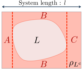
Figure 3: Multipartite correlations in the surface code. In the ground states of the Kitaev model on sphere, it has no multi-party correlation (or contains only low-degree of correlations), but collective properties of the low-degree of correlations induce multi-party correlation when we look at reduced region of the system, say $L^{{\rm c}}$. Indeed, if we split the region $L^{{\rm c}}$ into $A$, $B$ and $C$, we obtain non-trivial value of the topological entanglement entropy.

The notion of irreducible multipartite correlation has been first introduced in Ref. Linden et al. (2002) to characterize the multipartite correlations in a quantum state. It was noted recently that such notion is equivalent to the topological entanglement entropy if the state has zero-correlation length Kato et al. (2016). As explained in Refs Zhou (2008); Liu et al. (2016), we have two kinds of multipartite correlation, which we refer to as ‘effective multiparty correlations’, distinct from ‘inherent multipartite correlations.’ The topological entanglement entropy cannot distinguish them. We have:

i) The degenerate topological order, as that one of the toric code on a torus, has genuine multiparty correlation of the ‘inherent’ type involving $\mathcal{O}(l)$ spins ($l$: the system length).

ii) The non-degenerate topological order, as the toric code on the sphere, has low degree of inherent multiparty correlations involving $\mathcal{O}(1)$ spins, but have the ‘effective’ type involving $\mathcal{O}(l)$ spins.

In other words, a non-vanishing topological entanglement entropy in non-degenerate topological order arises just because of such multiparty low-degree correlations. There, we have no high-degree multiparty correlations if we look at the total system; in contrast, multiparty correlations of $\mathcal{O}(l)$ can be effectively induced by tracing out some finite suregions (See Fig. 3) Liu et al. (2016). Such a conditional many-body correlations can appear in short-range entangled state Bravyi ; Haah or even in classical models Galla and Gühne (2012).

In this way, we can see qualitative difference between the degenerate and the non-degenerate topological orders in terms of the irreducible multiparty correlation, which results in LR of the surface code and non-LR of the toric code. Being our approach able to detect such ‘fine structure’ in the nature of the multipartite correlations, the LR tells degenerate topological order apart from non-degenerate topological order.

Appendix D Symmetry-restricted Local Reversibility

Symmetry restricted LR states (SRL) can be introduced along very similar lines used in Sec. II. Let’s consider a given Hamiltonian $H$ enjoying a global symmetry $G$; let $|\psi\rangle$ be the ground state of $H$. We say that the state $|\psi\rangle$ is SLR iff the property (1) holds with a $q$-local operator $R$ enjoying the same symmetry group of the Hamiltonian: $[R,G]=0$.

Here we present an example of states which are not SLR. Cluster states provide an example of SPTO. The 1D cluster states Son et al. (2011) are the ground states of the Hamiltonian

$$H_{C}=\sum_{i=1}^{L}\sigma_{i-1}^{x}\sigma_{i}^{z}\sigma_{i+1}^{x}\,,$$ (28)

which enjoys a global symmetry $Z_{2}\times Z_{2}$ Son et al. (2012). With the boundary conditions $\sigma_{0}^{x}=\sigma_{L+1}^{x}={\mathbb{I}}$, the ground space of $H_{C}$ is unique with a spectral gap. For $\sigma_{0}^{x}=\sigma_{L+1}^{x}=0$, in contrast, the ground space is four-fold degenerate because the two stabilizers (out of $L$) $\sigma_{0}^{x}\sigma_{1}^{z}\sigma_{2}^{x}$ and $\sigma_{L-1}^{x}\sigma_{L}^{z}\sigma_{L+1}^{x}$ can be fixed at will Son et al. (2012). Let {$|\Omega_{\alpha}\rangle,\alpha=0,1,2,3\}$ be spanning the ground state manifold. Due to the symmetry-protected topological order of the system, it follows that the ground states $|\Omega_{\alpha}\rangle$ cannot be distinguished by any local operator $o_{X}$ in $Z_{2}\times Z_{2}$:

$$\langle\Omega_{\alpha}|o_{X}|\Omega_{\alpha}\rangle=\langle\Omega_{\beta}|o_{X}|\Omega_{\beta}\rangle,\quad{\rm and}\quad\langle\Omega_{\alpha}|o_{X}|\Omega_{\beta}\rangle=0.$$ (29)

with $|X|\leq cN$ ($c=\mathcal{O}(1)$). Using these conditions, the symmetry-restricted non-LR of $|\Omega_{\alpha}\rangle$ follows from the same arguments that were used in the proof of the non-LR of the toric code.

Appendix E Critical exponents

Here, we derive inequality (9) for the critical exponents $z$, $\eta$, $\gamma$ and $\nu$ under the scaling ansatz (31) Vojta (2003); Continentino (1994). Recall that we are considering a local Hamiltonian system at $T=0$ which is driven towards critically, and let $A=\sum_{i}a_{i}$, where $a_{i}$ are single particle operators that correspond to a local order parameter (e.g., spin localized at site $i$ leading to the magnetization along a given axes). Our starting point is inequality (8), namely

$$\delta E\cdot(\Delta A)^{2}\leq{\rm const}\cdot N\,.$$ (30)

We first define the variance $(\Delta A_{t})^{2}$ which depends on time as $(\Delta A_{t})^{2}:=\big{\langle}\big{(}A(t)-\langle A\rangle\big{)}\cdot\big{(}\langle A-\langle A\rangle\big{)}\big{\rangle}$, where $A(t)=e^{-iHt}Ae^{iHt}$. The variance $(\Delta A_{t})^{2}$ reduces to the summation of the correlation functions:

$$(\Delta A_{t})^{2} =\sum_{i,j=1}^{N}\langle a_{i}(t)a_{j}\rangle-\langle a_{i}\rangle\langle a_{j}\rangle:=\sum_{i,j=1}^{N}C_{i,j}(t),$$

where $a_{i}(t):=e^{-iHt}a_{i}e^{iHt}$ for $i=1,2,\ldots N$. Note that $(\Delta A_{t=0})^{2}$ is equal to $(\Delta A)^{2}=\langle A^{2}\rangle-\langle A\rangle^{2}$. In the following, we denote $C_{i,j}(t)=C({\bm{r}},t)$ under the assumption of the translation symmetry.

Now, we adopt the following scaling ansatz Continentino (1994):

$$S({\bm{q}},\omega;\xi)=\xi^{2-\eta}D({\bm{q}}\xi,\omega\xi^{z}),$$ (31)

where $\xi$ is the correlation length and $S({\bm{q}},\omega;\xi)$ is the spatial-temporal Fourier component of $C({\bm{r}},t)$, namely

$$S({\bm{q}},\omega;\xi) =\int_{{\bm{r}}}\int_{t}C({\bm{r}},t)e^{-i({\bm{q}}\cdot{\bm{r}}+\omega t)}d{\bm{r}}dt.$$ (32)

We also define $S({\bm{q}};\xi)$ as

$$S({\bm{q}};\xi)=\frac{1}{2\pi}\int_{-\infty}^{\infty}S({\bm{q}},\omega;\xi)d\omega.$$ (33)

We can see that the static fluctuation $(\Delta A_{t=0})^{2}$ is equal to $NS({\bm{q}}=0;\xi)$ by expanding $S({\bm{q}}=0;\xi)$.

We then obtain the scaling of $S({\bm{q}}=0;\xi)\propto\xi^{2-\eta-z}$ by taking the scaling (31) for $S({\bm{q}},\omega;\xi)$, and hence we have $(\Delta A_{t=0})^{2}/N\propto\xi^{2-\eta-z}$. We also have the scaling of the energy gap as $\delta E_{0}\propto\xi^{-z}$ Continentino (1994) by the use of the dynamical critical exponent $z$. At a critical point, where the correlation length is as large as the system length, the inequality (30) reduces to

$$-z\leq-(2-\eta-z)$$ (34)

in the infinite volume limit ($N\to\infty$). This reduces to the inequality (9) in the main manuscript.

We close the section applying inequality (8) to a system with long-range interactions: the Lipkin-Meshcov-Glick model $H_{\rm LMG}=-\frac{\lambda}{N}\sum_{i<j}(\sigma_{i}^{x}\sigma_{j}^{x}+\gamma\sigma_{i}^{y}\sigma_{j}^{y})+\sum_{i=1}^{N}h\sigma_{i}^{x}$ with $|\gamma|\leq 1$. At the critical point $\lambda=|h|$, we have the scaling Dusuel and Vidal (2004) of $\delta E\propto N^{-1/3}$ and $(\Delta M_{x})^{2}\propto N^{4/3}$, where $M_{x}$ is the magnetization in the $x$ direction, $M_{x}=\sum_{i=1}^{N}\sigma_{i}^{x}$. Thus, the spectral gap and the fluctuation can give the non-trivial sharp upper bounds to each other.

Appendix F The quality of the mean-field approximation

Let $|\Omega\rangle$ be the unique ground state of a gapped local Hamiltonian, and let $\rho_{ij},\rho_{i},\rho_{j}$ be its two-particles and one-particles reduced density matrices. We want to estimate the error of the mean-field approximation $\rho_{ij}\to\rho_{i}\otimes\rho_{j}$ by proving inequality (10) in the main text. For simplicity, we set $i=1$ and show that

$$\sum_{j\in L}\|\rho_{1,j}-\rho_{1}\otimes\rho_{j}\|\leq{\rm const}\cdot\sqrt{|L|/\delta E}\,.$$ (35)

First, note that we can always find a set of $d^{2}$ projectors $\{P_{1}^{(m)}\}$ onto the spin $i=1$ that satisfy

$$\|\rho_{1,j}-\rho_{1}\otimes\rho_{j}\|\leq\sum_{m=1}^{d^{2}}\|P_{1}^{(m)}(\rho_{1,j}-\rho_{1}\otimes\rho_{j})P_{1}^{(m)}\|\,,$$ (36)

where $d$ is the local spin dimension. For example, in the case of spin-1/2 systems ($d=2$), we can take $P_{1}^{(1)}=|0_{1}\rangle\langle 0_{1}|$, $P_{1}^{(2)}=|1_{1}\rangle\langle 1_{1}|$, $P_{1}^{(3)}=|+_{1}\rangle\langle+_{1}|$, $P_{1}^{(4)}=|-_{1}\rangle\langle-_{1}|$, with $|\pm_{1}\rangle:=(|0_{1}\rangle\pm|1_{1}\rangle)/\sqrt{2}$. Indeed, defining $\delta\rho_{1,j}:=\rho_{1,j}-\rho_{1}\otimes\rho_{j}$, we get

$$\|\delta\rho_{1,j}\| \leq\|\langle 0_{1}|\delta\rho_{1,j}|0_{1}\rangle\|+\|\langle 1_{1}|\delta\rho_{1,j}|1_{1}\rangle\|+\|\langle 0_{1}|\delta\rho_{1,j}|1_{1}\rangle+\langle 1_{1}|\delta\rho_{1,j}|0_{1}\rangle\|$$

$$=\|\langle 0_{1}|\delta\rho_{1,j}|0_{1}\rangle\|+\|\langle 1_{1}|\delta\rho_{1,j}|1_{1}\rangle\|+\|\langle+_{1}|\delta\rho_{1,j}|+_{1}\rangle-\langle-_{1}|\delta\rho_{1,j}|-_{1}\rangle\|$$

$$\leq\|\langle 0_{1}|\delta\rho_{1,j}|0_{1}\rangle\|+\|\langle 1_{1}|\delta\rho_{1,j}|1_{1}\rangle\|+\|\langle+_{1}|\delta\rho_{1,j}|+_{1}\rangle\|+\|\langle-_{1}|\delta\rho_{1,j}|-_{1}\rangle\|\,.$$

The proof for higher $d$ follows the same lines.

Summing inequality (36) over all $j\in L$ gives

$$\sum_{j\in L}\|\rho_{1,j}-\rho_{1}\otimes\rho_{j}\|\leq\sum_{m=1}^{d^{2}}\sum_{j\in L}\|P_{1}^{(m)}(\rho_{1,j}-\rho_{1}\otimes\rho_{j})P_{1}^{(m)}\|\,.$$

To prove inequality (35), we will show an upper bound of $\sum_{j\in L}\|P_{1}^{(m)}(\rho_{1,j}-\rho_{1}\otimes\rho_{j})P_{1}^{(m)}\|$ for arbitrary $m$.

Defining $\rho_{j}^{(m)}:=\mathop{\rm Tr}\nolimits_{1}(P_{1}^{(m)}\rho_{1,j}P_{1}^{(m)})$, where $\mathop{\rm Tr}\nolimits_{i}(\cdots)$ is the partial trace over the $i$th spin, we get

$$P_{1}^{(m)}(\rho_{1,j}-\rho_{1}\otimes\rho_{j})P_{1}^{(m)}=P_{1}^{(m)}\otimes\bigl{(}\rho_{j}^{(m)}-\langle\Omega|P_{1}^{(m)}|\Omega\rangle\cdot\rho_{j}\bigr{)}\,.$$

Clearly, $\|P_{1}^{(m)}\otimes\bigl{(}\rho_{j}^{(m)}-\langle\Omega|P_{1}^{(m)}|\Omega\rangle\cdot\rho_{j}\bigr{)}\|=\|\rho_{j}^{(m)}-\langle\Omega|P_{1}^{(m)}|\Omega\rangle\cdot\rho_{j}\|$. Moreover, there always exists a rank-1 projector $P_{j}^{(m)}$ such that

$$\|\rho_{j}^{(m)}-\langle\Omega|P_{1}^{(m)}|\Omega\rangle\cdot\rho_{j}\|=s_{j}^{(m)}\cdot\mathop{\rm Tr}\nolimits\Bigl{[}P_{j}^{(m)}\bigl{(}\rho_{j}^{(m)}-\langle\Omega|P_{1}^{(m)}|\Omega\rangle\cdot\rho_{j}\bigr{)}\Bigr{]}\,,$$

where $s_{j}^{(m)}:=\textrm{sign}\Bigl{\{}\mathop{\rm Tr}\nolimits\bigl{[}P_{j}^{(m)}(\rho_{j}^{(m)}-\langle\Omega|P_{1}^{(m)}|\Omega\rangle\cdot\rho_{j})\bigr{]}\Bigr{\}}$. Therefore,

$$\|P_{1}^{(m)}(\rho_{1,j}-\rho_{1}\otimes\rho_{j})P_{1}^{(m)}\| =s_{j}^{(m)}\cdot\mathop{\rm Tr}\nolimits\Bigl{[}P_{j}^{(m)}\bigl{(}\rho_{j}^{(m)}-\langle\Omega|P_{1}^{(m)}|\Omega\rangle\cdot\rho_{j}\bigr{)}\Bigr{]}$$

$$=s_{j}^{(m)}\cdot\bigl{[}\langle\Omega|P_{1}^{(m)}P_{j}^{(m)}|\Omega\rangle-\langle\Omega|P_{1}^{(m)}|\Omega\rangle\cdot\langle\Omega|P_{j}^{(m)}|\Omega\rangle\bigr{]}\,.$$

We now define the additive operator

$$A^{(m)}:=\sum_{j\in L}s_{j}^{(m)}\cdot P_{j}^{(m)}\,.$$

Then from the above calculation,

$$\sum_{j\in L}\|P_{1}^{(m)}(\rho_{1,j}-\rho_{1}\otimes\rho_{j})P_{1}^{(m)}\|=\langle\Omega|P_{1}^{(m)}A^{(m)}|\Omega\rangle-\langle\Omega|P_{1}^{(m)}|\Omega\rangle\cdot\langle\Omega|A^{(m)}|\Omega\rangle\,.$$

But

$$\langle\Omega|P_{1}^{(m)}A^{(m)}|\Omega\rangle-\langle\Omega|P_{1}^{(m)}|\Omega\rangle\cdot\langle\Omega|A^{(m)}|\Omega\rangle =\langle\Omega|P_{1}^{(m)}\cdot\Big{[}A^{(m)}|\Omega\rangle-\langle\Omega|A^{(m)}|\Omega\rangle|\Omega\rangle\Big{]}$$

$$\leq\|P^{(m)}_{1}|\Omega\rangle\|\cdot\|A^{(m)}|\Omega\rangle-\langle\Omega|A^{(m)}|\Omega\rangle|\Omega\rangle\|\,,$$

and as $\|A^{(m)}|\Omega\rangle-\langle\Omega|A^{(m)}|\Omega\rangle|\Omega\rangle\|=\Delta A^{(m)}$, we conclude that

$$\sum_{j\in L}\|P_{1}^{(m)}(\rho_{1,j}-\rho_{1}\otimes\rho_{j})P_{1}^{(m)}\| \leq\Delta A^{(m)}\leq{\rm const}\cdot\sqrt{|L|/\delta E}\,.$$

Here, the last inequality comes from the inequality (8) in the main text, which applies in this case since $A^{(m)}$ is an additive operator on $L$. Combining this with inequality (36) completes the proof.

Optimality of the bound
When $\delta E=\mathcal{O}(1)$, inequality (35) reduces to

$$\sum_{j\in L}\|\rho_{1,j}-\rho_{1}\otimes\rho_{j}\|\leq{\rm const}\cdot\sqrt{|L|}\,.$$ (37)

We can ensure that this upper bound is qualitatively optimal by considering the state

$$\frac{1}{\sqrt{2}}|0_{1}\rangle|0_{2}0_{3}\cdots 0_{N}\rangle+\frac{1}{\sqrt{2}}|1_{1}\rangle|{\rm W}_{2,\ldots,N}\rangle\,,$$ (38)

where $|{\rm W}_{2,\ldots,N}\rangle$ is the W state for the spins $2,3,\ldots,N$. We note that this state satisfies inequality $(\Delta A)^{2}\leq\mathcal{O}(|L|)$  Shimizu and Morimae (2005), which is equivalent to the inequality (8) in the case of $\delta E=\mathcal{O}(1)$. Interestingly, the state in (38) also gives the upper limit of the monogamy inequality of the entanglement Osborne and Verstraete (2006).

References

- Wen (2004) X.-G. Wen, Quantum Field Theory of Many-body Systems from the Origin of Sound to an Origin of Light and Electrons by Xiao-Gang Wen. Published in the United States by Oxford University Press Inc., New York, 2004. ISBN 019853094. 1 (2004).
- Chen et al. (2010) X. Chen, Z.-C. Gu, and X.-G. Wen, Phys. Rev. B 82, 155138 (2010).
- Hayden et al. (2006) P. Hayden, W. D. Leung, and A. Winter, Communications in Mathematical Physics 265, 95 (2006).
- Osborne (2012) T. J. Osborne, Reports on Progress in Physics 75, 022001 (2012), arXiv:arXiv:1106.5875 [quant-ph] .
- Hastings (2004) M. B. Hastings, Phys. Rev. B 69, 104431 (2004), arXiv:cond-mat/0305505 .
- Hastings and Koma (2006) M. B. Hastings and T. Koma, Communications in Mathematical Physics 265, 781 (2006).
- Nachtergaele and Sims (2006) B. Nachtergaele and R. Sims, Communications in Mathematical Physics 265, 119 (2006).
- Eisert et al. (2010) J. Eisert, M. Cramer, and M. B. Plenio, Rev. Mod. Phys. 82, 277 (2010), arXiv:0808.3773 .
- Amico et al. (2008) L. Amico, R. Fazio, A. Osterloh, and V. Vedral, Rev. Mod. Phys. 80, 517 (2008).
- Hastings (2007a) M. B. Hastings, Journal of Statistical Mechanics: Theory and Experiment 2007, P08024 (2007a), arXiv:0705.2024 .
- Arad et al. (2012) I. Arad, Z. Landau, and U. Vazirani, Phys. Rev. B 85, 195145 (2012).
- Arad et al. (2013) I. Arad, A. Kitaev, Z. Landau, and U. Vazirani, ArXiv:1301.1162 (2013), arXiv:1301.1162 .
- Cho (2014) J. Cho, Phys. Rev. Lett. 113, 197204 (2014).
- Brandão and Horodecki (2013) F. G. Brandão and M. Horodecki, Nature Physics 9, 721 (2013).
- Arad et al. (2016a) I. Arad, Z. Landau, U. Vazirani, and T. Vidick, arXiv preprint arXiv:1602.08828 (2016a), arXiv:1602.08828 .
- Verstraete et al. (2008) F. Verstraete, V. Murg, and J. I. Cirac, Advances in Physics 57, 143 (2008).
- Chen et al. (2011) X. Chen, Z.-C. Gu, and X.-G. Wen, Phys. Rev. B 84, 235128 (2011).
- Ge and Eisert (2016) Y. Ge and J. Eisert, New Journal of Physics 18, 083026 (2016), arXiv:1411.2995 .
- Hoory et al. (2006) S. Hoory, N. Linial, and A. Wigderson, Bulletin of the American Mathematical Society 43, 439 (2006).
- Kempe et al. (2006) J. Kempe, A. Kitaev, and O. Regev, SIAM Journal on Computing 35, 1070 (2006), arXiv:quant-ph/0406180 .
- Hastings (2007b) M. B. Hastings, Phys. Rev. B 76, 035114 (2007b).
- Aharonov et al. (2013) D. Aharonov, I. Arad, and T. Vidick, Acm sigact news 44, 47 (2013), arXiv:1309.7495 .
- Chen et al. (2013) X. Chen, Z.-C. Gu, Z.-X. Liu, and X.-G. Wen, Phys. Rev. B 87, 155114 (2013).
- Shimizu and Morimae (2005) A. Shimizu and T. Morimae, Phys. Rev. Lett. 95, 090401 (2005).
- Fröwis and Dür (2012) F. Fröwis and W. Dür, New Journal of Physics 14, 093039 (2012).
- Haldane (1983) F. D. M. Haldane, Phys. Rev. Lett. 50, 1153 (1983).
- Affleck et al. (1987) I. Affleck, T. Kennedy, E. H. Lieb, and H. Tasaki, Phys. Rev. Lett. 59, 799 (1987).
- Lipkin et al. (1965) H. Lipkin, N. Meshkov, and A. Glick, Nuclear Physics 62, 188 (1965).
- Cui et al. (2013) J. Cui, L. Amico, H. Fan, M. Gu, A. Hamma, and V. Vedral, Phys. Rev. B 88, 125117 (2013).
- Kitaev (2003) A. Kitaev, Annals of Physics 303, 2 (2003).
- Levin and Wen (2005) M. A. Levin and X.-G. Wen, Phys. Rev. B 71, 045110 (2005).
- Arad et al. (2016b) I. Arad, T. Kuwahara, and Z. Landau, Journal of Statistical Mechanics: Theory and Experiment 2016, 033301 (2016b), arXiv:1406.3898 .
- Raussendorf and Briegel (2001) R. Raussendorf and H. J. Briegel, Phys. Rev. Lett. 86, 5188 (2001).
- Briegel and Raussendorf (2001) H. J. Briegel and R. Raussendorf, Phys. Rev. Lett. 86, 910 (2001).
- Hein et al. (2004) M. Hein, J. Eisert, and H. J. Briegel, Phys. Rev. A 69, 062311 (2004).
- Hastings (2011) M. B. Hastings, Phys. Rev. Lett. 107, 210501 (2011), arXiv:1106.6026 .
- Freedman and Hastings (2014) M. H. Freedman and M. B. Hastings, Quantum Information & Computation 14, 144 (2014).
- Hastings (2012) M. B. Hastings, “Locality in quantum systems,” in Quantum Theory from Small to Large Scales: Lecture Notes of the Les Houches Summer School: Volume 95, August 2010 (Oxford Scholarship Online, 2012) p. see pg. 24 on arXiv version arXiv:1008.5137, arXiv:1008.5137 .
- Zhou (2008) D. L. Zhou, Phys. Rev. Lett. 101, 180505 (2008).
- Kato et al. (2016) K. Kato, F. Furrer, and M. Murao, Phys. Rev. A 93, 022317 (2016).
- Liu et al. (2016) Y. Liu, B. Zeng, and D. L. Zhou, New Journal of Physics 18, 023024 (2016), arXiv:1402.4245 .
- Son et al. (2012) W. Son, L. Amico, and V. Vedral, Quantum Information Processing 11, 1961 (2012).
- Hoeffding (1963) W. Hoeffding, Journal of the American Statistical Association 58, 13 (1963).
- Kuwahara (2016) T. Kuwahara, Journal of Statistical Mechanics: Theory and Experiment 2016, 053103 (2016).
- Continentino (1994) M. A. Continentino, Physics Reports 239, 179 (1994).
- Vojta and Schmalian (2005) T. Vojta and J. Schmalian, Phys. Rev. Lett. 95, 237206 (2005).
- Dusuel and Vidal (2004) S. Dusuel and J. Vidal, Phys. Rev. Lett. 93, 237204 (2004).
- Brandão and Harrow (2013) F. G. Brandão and A. W. Harrow, in Proceedings of the Forty-fifth Annual ACM Symposium on Theory of Computing, STOC ’13 (ACM, New York, NY, USA, 2013) pp. 871–880.
- Osterloh and Schützhold (2015) A. Osterloh and R. Schützhold, Phys. Rev. B 91, 125114 (2015).
- Brandão and Cramer (2015) F. G. S. L. Brandão and M. Cramer, ArXiv:1502.03263 (2015), arXiv:arXiv:1502.03263 [quant-ph] .
- Lubasch et al. (2014a) M. Lubasch, J. I. Cirac, and M.-C. Bañuls, Phys. Rev. B 90, 064425 (2014a), arXiv:1405.3259 .
- Lubasch et al. (2014b) M. Lubasch, J. I. Cirac, and M.-C. Bañuls, New Journal of Physics 16, 033014 (2014b), arXiv:1311.6696 .
- Anshu et al. (2016) A. Anshu, I. Arad, and A. Jain, arXiv preprint arXiv:1603.06049 (2016), arXiv:1603.06049 .
- Schwarz et al. (2016) M. Schwarz, O. Buerschaper, and J. Eisert, arXiv preprint arXiv:1606.06301 (2016), arXiv:1606.06301 .
- Facchi et al. (2011) P. Facchi, G. Florio, S. Pascazio, and F. V. Pepe, Phys. Rev. Lett. 107, 260502 (2011).
- Abramowitz and Stegun (1972) M. Abramowitz and I. A. Stegun, Handbook of mathematical functions: with formulas, graphs, and mathematical tables, 55 (Courier Dover Publications, 1972).
- Kitaev and Preskill (2006) A. Kitaev and J. Preskill, Phys. Rev. Lett. 96, 110404 (2006).
- Levin and Wen (2006) M. Levin and X.-G. Wen, Phys. Rev. Lett. 96, 110405 (2006).
- Linden et al. (2002) N. Linden, S. Popescu, and W. K. Wootters, Phys. Rev. Lett. 89, 207901 (2002).
- (60) S. Bravyi, unpublished .
- (61) J. Haah, Coogee’15, talk slide, 16page .
- Galla and Gühne (2012) T. Galla and O. Gühne, Phys. Rev. E 85, 046209 (2012).
- Son et al. (2011) W. Son, L. Amico, R. Fazio, A. Hamma, S. Pascazio, and V. Vedral, EPL (Europhysics Letters) 95, 50001 (2011).
- Vojta (2003) M. Vojta, Reports on Progress in Physics 66, 2069 (2003).
- Osborne and Verstraete (2006) T. J. Osborne and F. Verstraete, Phys. Rev. Lett. 96, 220503 (2006).