Complexity and self-organization in Turing

1 Introduction: “converting chemical information into a geometrical form”

Alan Turing’s celebrated paper “The Chemical Basis of Morphogenesis” [22] published in 1952 in the Philosophical Transactions of the Royal Society of London is a typical example of a pioneering and inspired work in the domain of mathematical modelling.

1. The paper presents a new key idea for solving an old problem. As Lionel Harrison said in his 1987 paper [6] “it is a theoretical preconception preceeding experience”.

2. It contains right away the germ of quite the whole theory associated to the new ideas.

3. Its forsightedness is striking. It anticipates by many years its experimental confirmations and mathematical developments.

The key idea is formulated from the outset in the first sentence:

“It is suggested that a system of chimical substances, called morphogens, reacting together and diffusing through a tissue, is adequate to account for the main phenomena of morphogenesis.”

Later (1953), Turing used a striking formulation (see below figure 2):

“It was suggested in Turing (1952) that this might be the main means by which the chemical information contained in the genes was converted into a geometrical form.”

Turing’s colleague Claude Wilson Wardlaw, a botanist at the Department of Cryptogamic Botany at Manchester University who wrote with Turing the paper “A diffusion reaction theory of morphogenesis in plants” [24], said in 1952 that Turing’s working hypothesis was that:

“a localized accumulation of gene-determined substances may be an essential prior condition [for cell differentiation].” (p. 40)

and that what is needed in addition to biochemistry for understanding emerging spatial forms in morphogenetic processes is a “patternized distribution of morphogenetic substances”. There exist many homologies of organization between different biological species and it must therefore exist general morphogenetics mechanisms largely independent of specific genes. As he claimed, “certain physical processes are of very general occurrence” (p. 46).

Wardlaw summarizes Turing’s key idea in the following way:

“In an embryonic tissue in which the metabolic substances may initially be distributed in a homogeneous manner, a regular, patternized distribution of specific metabolites may eventually result, thus affording the basis for the inception of morphological or histological patterns.” (p. 44)

So, for understanding how a spatial order can emerge from biochemical reactions genetically controlled – which, according to Turing, is the main problem of morphogenesis – Turing defines from the outset a form as a breaking of homogeneity of some spatially extended biological tissue and, therefore, as a breaking of the symmetries underlying such an homogeneity.

2 The framework

2.1 Turing diffusion-driven instability

The components of Turing’s theorization are the following. Inside the biological tissue under consideration, chimical reactions occur, which we will call internal chimical dynamics. In the spatial extension of this substrate, processes of spatial diffusion occur, which we will call external spatial dynamics. The key idea is that the coupling of these two very different kinds of dynamics can trigger, under certain conditions, morphogenetic processes, which can be mathematically modelled by using what are called since Turing reaction-diffusion differential equations. Why and how? Because the external spatial diffusion can destabilize, under certain conditions, the internal chimical equilibria.

We must emphasize the fact that the notion of diffusion-driven instabilities is to some extent paradoxical. Indeed, diffusion is a stabilizing process and therefore the idea amounts to posit that the coupling of two stabilities can induce an instability!

We will see that Turing assumes that there exists only one equilibrium of the internal chimical dynamics. A diffusion-induced instability could therefore make the chimical state diverge, but in general non-linearities of the equations bound such divergences. Another possibility would be that there exist several equilibria. Then Turing instabilities would induce bifurcations from one equilibrium state to another one. It is this idea that has been worked out in the late 1960s by René Thom [20], [21] to explain also morphogenesis.

2.2 Turing’s objective

Today, reaction-diffusion equations are mainly used to explain the formation of patterns in material substrates. But Turing’s objective was deeper and more ambitious and concerned embryogenesis. As he claimed in his Introduction,

“The purpose of this paper is to discuss a possible mechanism by which the genes of a zygote may determine the anatomical structure of the resulting organism.” (p. 37)

As this general objective was too ambitious, he assumed many simplifications. The first simplification was to eliminate any direct reference to specific genes and to reduce the internal chemical dynamics to reaction equations between concentrations of morphogens. As explains Philip Maini in [9], a morphogen is

“a chemical to which cells respond by differentiating in a concentration-dependent way.”

Turing was inspired by what Waddington [25] called “form producers” or “evocators”. Morphogens are controlled by genes which catalize their production, but, contrary to genes, they can diffuse in the developing tissues and carry the positional information (e.g. in the sense of Wolpert) which is needed for morphogenesis.

The second simplification made by Turing was to eliminate the mechano-chemical aspects of embryogenesis, although he was aware of their importance during the development. These aspects will be worked out later by specialists such as George Oster and James Murray

But, even so drastically simplified, the search for good mathematical models remains a

“a problem of formidable mathematical complexity” (p. 38).

In fact, it seems that Turing was looking for a kind of universal equation for morphogenesis. In his last paper “Morphogen theory of phyllotaxis”, which remained unpublished because of his suicide and is kept at the King’s College Archives, he proposed the equation

$$\frac{d\Gamma_{m}}{dt}=\mu_{m}\nabla^{2}\Gamma_{m}+f_{m}\left(\Gamma_{1},\cdots,\Gamma_{M}\right)$$

where the $\Gamma_{m}$ are the respective concentrations of the $M$ morphogens, $\nabla^{2}$ the spatial Laplacian, that is the diffusion operator, the $\mu_{m}$ the diffusibility coefficients, and the $f_{m}$ the reaction equations (see figure 1)

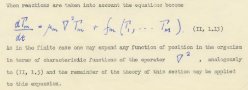
Figure 1: Turing’s general equation for morphogenesis.

The point was that, when you vary the $f_{m}$ and the $\mu_{m}$, the solutions of such a universal equation can be extremely diverse (see figure 2). Hence the idea that, as with Newton’s equation for Mechanics, it could be possible to classify a lot of very different kinds of forms using the same general equation.

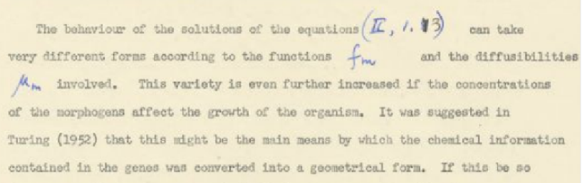
Figure 2: Turing’s anticipation of the richness of the general equation for morphogenesis.

Indeed, we can vary three classes of parameters:

1. For the chemical part, the eigenvalues provided by the spectral analysis of the linearized system of the $f_{m}$.

2. The diffusibility coefficients $\mu_{m}$.

3. For the geometrical part, the eigenfunctions of the Laplacian operator (harmonic analysis).

2.3 Turing’s foresightedness

In his 1990 paper “Turing’s theory of morphogenesis. Its influence on modelling biological pattern and form” [15], James Murray claims that Turing’s 1952 paper is “one of the most important papers in theoretical biology of this century” (p. 119). Indeed,

“What is astonishing about Turing’s seminal paper is that, with very few exceptions, it took the mathematical world more than 20 years to realise the wealth of fascinating problems posed by his theory. What is even more astonishing is that it was closer to 30 years before a significant number of experimental biologists took serious notice of its implications and potential applications in developmental biology, ecology and epidemiology.” (p. 121)

These inspired anticipations proved to be exact in chemistry. There exist today a lot of models of chimical reaction-diffusion phenomena: clocks, travelling waves, etc. Their analysis constitutes a rapidly expanding research domain while, at Turing’s time, no empirical example was known. Turing discovered theoretically the basic phenomenon and was the first to compute simulations on the computer he had himself constructed at Manchester. In embryogenesis, the exact limits of validity of Turing model are still under discussion.

3 The context

3.1 The bibliography

It is interesting to look at Turing’s bibliography, which is very short. First, it includes two books which are not really used, the Theory of Elasticity and Magnetism of James Jeans (1927) and The permeability of natural membranes of Hugh Dawson and James Danielli (1943). Then, it cites a fundamental paper of Leonor Michaelis and Maud Menten (1913) on Die Kinetik der Invertinwirkung [13] whose pioneering mathematical model is typical of the internal chimical dynamics used by Turing. Finally, there are three masterpieces on embryology and morphogenesis: Charles Manning Child’s “summa” Patterns and problems of development (1941), Sir D’Arcy Thompson’s masterpiece On Growth and Form (1942) [1] and Conrad Hal Waddington’s key work on Organizers and Genes (1940) [25]. Introduced by Hans Spemann, “organizers” were thought to be the cause of the embryological induction observed when the tissues of some part of an embryo (e.g. a leg) were transplanted in another part (e.g. the head). The idea (much speculative at that time) was that there must exist chemical signals triggering cellular differenciations. It is in the second part of this work that Waddington assumed that, through morphogens, gene concentrations could be important for cellular differenciation and that the developmental units of an organism are “morphogenetic fields”.

3.2 The kinetic model

Building on previous very precise numerical experimental data collected by Victor Henri (1903), the Michaelis-Menten model of the kinetics of invertase enzyme (1913) was the first to explain the catalysis of the hydrolysis of sucrose into glucose and fructose. Let $E$ be an enzyme bounding with a substrate $S$ to give a complex $ES$ which converts itself into a product $P$ through a chain of two elementary chemical reactions:

$$E+S\overset{k_{1}}{\underset{k_{2}}{\rightleftarrows}}ES\overset{k_{3}}{\rightarrow}E+P$$

where the $k_{i}$ are the rate constants of the reactions. Let us denote by $\left[X\right]$ the concentration of $X$. Then the law of mass action saying that a reaction rate is proportional to the product of the concentrations of the reactants implies the system of nonlinear differential equations:

$$\left\{\begin{array}[]{l}\overset{\cdot}{\left[S\right]}=-k_{1}\left[E\right]\left[S\right]+k_{2}\left[ES\right]\\ \overset{\cdot}{\left[E\right]}=-k_{1}\left[E\right]\left[S\right]+k_{2}\left[ES\right]+k_{3}\left[ES\right]\\ \overset{\cdot}{\left[ES\right]}=k_{1}\left[E\right]\left[S\right]-k_{2}\left[ES\right]-k_{3}\left[ES\right]\\ \overset{\cdot}{\left[P\right]}=k_{3}\left[ES\right]\end{array}\right.$$

where the relation $\overset{\cdot}{\left[E\right]}+\overset{\cdot}{\left[ES\right]}=0$ implies the conservation law $\left[E\right]+\left[ES\right]=E_{0}=$ constant. Under an hypothesis of adiabaticity according to which the equilibrium between $S$ and $ES$ is “instantaneous”, that is $\overset{\cdot}{\left[S\right]}=0$, then $k_{1}\left[E\right]\left[S\right]=k_{2}\left[ES\right]$, $\left[ES\right]=\frac{k_{1}}{k_{2}}\left[E\right]\left[S\right]=\frac{k_{1}}{k_{2}}\left[S\right]\left(E_{0}-\left[ES\right]\right)$, $\left[ES\right]\left(1+\frac{k_{1}}{k_{2}}\left[S\right]\right)=\frac{k_{1}}{k_{2}}\left[S\right]E_{0}$ and

$$\left[ES\right]=\frac{k_{1}}{k_{2}}\left[S\right]E_{0}\left(\frac{1}{\left(1+\frac{k_{1}}{k_{2}}\left[S\right]\right)}\right)=\left[S\right]E_{0}\frac{1}{K}\left(\frac{1}{\left(1+\frac{1}{K}\left[S\right]\right)}\right)=\frac{E_{0}\left[S\right]}{K+\left[S\right]}$$

with $K=\frac{k_{2}}{k_{1}}$, and therefore

$$\overset{\cdot}{\left[P\right]}=k_{3}\frac{E_{0}\left[S\right]}{K+\left[S\right]}$$

4 Turing’s numerical example

So, Turing start with morphogens diffusing and reacting inside a tissue. Diffusion flows from regions of strong concentrations towards regions of weak concentrations with a velocity proportional to the gradients of the concentrations and to the diffusibility coefficients. According to the law of mass action, reaction rates are proportional to the product of concentrations. Hence a huge variety of nonlinear differential equations.

Turing gives several examples and develop one of them in minute detail in his §10 “A numerical example”. He considers a ring of $N=20$ cells and two morphogens $X$ and $Y$ and makes several numerical assumptions on their size, the diffusibility constants, the permeability of membranes (it is here that the reference to Dawson-Danielli is used), etc. With great acuity, he argues that the system must be (thermodynamically) open and include a “fuel substance” $A$ providing it with energy through its degradation into another substance $B$.

“In order to maintain the wave pattern a continual supply of free energy is required. It is clear that this must be so since there is a continual degradation of energy through diffusion. This energy is supplied through the ‘fuel substances’ ($A$, $B$ in the last example), which are degraded into ‘waste products’.” (p. 65)

For modelling catalysis, Turing add three other substances $C$, $C^{\prime}$, and $W$.

It must be emphasized that it will be only thirty years later that open thermodynamical systems out of equilibrium will be systematically investigated (see e.g. Prigogine’s dissipative structures).

4.1 The internal chimical dynamics

The system of $7$ elementary reactions proposed by Turing is the following:

$$\begin{array}[]{llccl}\left[1\right]&Y+X\rightarrow W&&&\text{rate: }\frac{25}{16}XY\\ \left[2\right]&W+A\rightarrow 2Y+B&&&\begin{array}[]{l}\text{(instantly)}\\ A=1000=\text{constant (fuel substance)}\end{array}\\ \left[3\right]&2X\rightarrow W&&&\text{rate: }\frac{7}{64}X^{2}\\ \left[4\right]&A\rightarrow X&&&\text{rate: }\frac{1}{16}10^{-3}A=\frac{1}{16}\\ \left[5\right]&Y\rightarrow B&&&\text{rate: }\frac{1}{16}Y\\ \left[6\right]&Y+C\rightarrow C^{\prime}&&&\begin{array}[]{l}\text{(instantly)}\\ C=C^{\prime}=10^{-3}\left(1+\gamma\right)\end{array}\\ \left[7\right]&C^{\prime}\rightarrow X+C&&&\text{rate: }\frac{55}{32}10^{3}C^{\prime}=\frac{55}{32}\left(1+\gamma\right)\end{array}$$

So, $X$ converts into $Y$ at the rate $\frac{1}{32}\left[50XY+7X^{2}-55\left(1+\gamma\right)\right]$ (because of $\left[1\right]$, $\left[3\right]$, and $\left[7\right]$) while self-reproducing (because of $\left[4\right]$) at the constant rate $\frac{1}{16}$ and destroying $Y$ (because of $\left[5\right]$) at the rate $\frac{1}{16}Y$. So the kinetic equations for the time varying concentrations $X\left(t\right)$, $Y\left(t\right)$ of the morphogens $X$, $Y$ – i.e. the internal chimical dynamics – are

$$\left\{\begin{array}[]{l}\overset{\cdot}{X}=\frac{1}{32}\left[-50XY-7X^{2}+57+55\gamma\right]=f\left(X,Y\right)\\ \overset{\cdot}{Y}=\frac{1}{32}\left[50XY+7X^{2}-55-55\gamma-2Y\right]=g\left(X,Y\right)\end{array}\right.$$

where $57$ in the first equation is $55+2$ with $2$ coming from $\left[4\right]$ and $-2Y$ in the second equation comes from $\left[5\right]$.

4.2 Equilibria and linearization

A chemical internal equilibrium corresponds to values $\left(X_{e},Y_{e}\right)$ such that $f\left(X_{e},Y_{e}\right)=0$ and $g\left(X_{e},Y_{e}\right)=0$. For $\gamma=0$ the system is

$$\left\{\begin{array}[]{l}\overset{\cdot}{X}=\frac{1}{32}\left[-50XY-7X^{2}+57\right]=f\left(X,Y\right)\\ \overset{\cdot}{Y}=\frac{1}{32}\left[50XY+7X^{2}-55-2Y\right]=g\left(X,Y\right)\end{array}\right.$$

and an evident equilibrium is $X_{0}=Y_{0}=1$. Another is $X_{1}=-\frac{57}{7},Y_{1}=1$ but it is non physical since a concentration cannot be negative.

Then, Turing linearizes the system near the equilibrium $\left(X_{0},Y_{0}\right)$ and analyzes the stability of the linear system. The method was already well known at his time: the matrix of the linearized system is the Jacobian $J_{0}$ of $\left\{f,g\right\}$ at $\left(X_{0},Y_{0}\right)$ and the stability depends upon the fact that the real part of all eigenvalues $\lambda$ of $J_{0}$ are $<0$. Let us briefly remind non mathematicians of it. It is immediate to compute $J_{0}$ for $\gamma=0$:

$$J_{0}=\left(\begin{array}[]{cc}\frac{\partial f}{\partial X}&\frac{\partial f}{\partial Y}\\ \frac{\partial g}{\partial X}&\frac{\partial g}{\partial Y}\end{array}\right)$$

and, as

$$\left\{\begin{array}[]{l}\frac{\partial f}{\partial X}=a=\frac{1}{32}\left[-50Y_{0}-14X_{0}\right]=-2\\ \frac{\partial f}{\partial Y}=b=\frac{1}{32}\left[-50X_{0}\right]=-\frac{25}{16}=-1.5625\\ \frac{\partial g}{\partial X}=c=\frac{1}{32}\left[50Y_{0}+14X_{0}\right]=2\\ \frac{\partial g}{\partial Y}=d=\frac{1}{32}\left[50X_{0}-2\right]=\frac{48}{32}=\frac{3}{2}=1.5\end{array}\right.$$

we get

$$J_{0}=\left(\begin{array}[]{cc}-2&-\frac{25}{16}\\ 2&\frac{3}{2}\end{array}\right)$$

In a small neighbourhood of $\left(X_{0},Y_{0}\right)$ we can write $X=X_{0}+x$, $Y=Y_{0}+y$ and write at first order

$$\left(\begin{array}[]{c}\dot{x}\\ \dot{y}\end{array}\right)=J_{0}\left(\begin{array}[]{c}x\\ y\end{array}\right),~{}\text{i.e. }\left\{\begin{array}[]{l}\dot{x}=ax+by\\ \dot{y}=cx+dy\end{array}\right.$$

As the system is linear, we look at solutions of the form

$$\left(\begin{array}[]{c}x\left(t\right)\\ y\left(t\right)\end{array}\right)=e^{\lambda t}\left(\begin{array}[]{c}x_{0}\\ y_{0}\end{array}\right)$$

where $\left(x_{0},y_{0}\right)$ is the state of the system at time $t=0$. They are straight trajectories on the line $\left(0,0\right)-\left(x_{0},y_{0}\right)$ with an exponential temporal law. Computing the derivatives in two different ways, we get

$$\left(\begin{array}[]{c}\dot{x}\\ \dot{y}\end{array}\right)=J_{0}\left(\begin{array}[]{c}x\\ y\end{array}\right)=\lambda e^{\lambda t}\left(\begin{array}[]{c}x_{0}\\ y_{0}\end{array}\right)=\lambda\left(\begin{array}[]{c}x\\ y\end{array}\right)$$

that is an equation linking $\lambda$ to $J_{0}$:

$$\left(J_{0}-\lambda I\right)\left(\begin{array}[]{c}x\\ y\end{array}\right)=0$$

If $\left(x_{0},y_{0}\right)\neq\left(0,0\right)$, then $\left(x,y\right)\neq\left(0,0\right)$ and this equation can be satisfied only if the determinant $\mathop{\mathrm{D}et}\left(J_{0}-\lambda I\right)$ vanishes. The equation $\mathop{\mathrm{D}et}\left(J_{0}-\lambda I\right)=0$ is called the characteristic equation of the linear system. It is a polynomial equation of degree $2$ which writes

$$\mathop{\mathrm{D}et}\left(\begin{array}[]{cc}a-\lambda&b\\ c&d-\lambda\end{array}\right) = 0$$

$$\lambda^{2}-\left(a+d\right)\lambda+ad-bc = 0$$

$$\lambda^{2}-\mathop{\mathrm{T}r}\left(J_{0}\right)\lambda+\mathop{\mathrm{D}et}\left(J_{0}\right) = 0$$

$$\lambda^{2}-S\lambda+P = 0$$

where the sum of diagonal terms $\mathop{\mathrm{T}r}\left(J_{0}\right)=a+d=S$, called the trace of the matrix $J_{0}$, gives the sum $S$ of the solutions and the determinant $\mathop{\mathrm{D}et}\left(J_{0}\right)$ of $J_{0}$ gives their product $P$. As the discriminant of the equation is $\Delta=S^{2}-4P=\mathop{\mathrm{T}r}\left(J_{0}\right)^{2}-4\mathop{\mathrm{D}et}\left(J_{0}\right)$, the solutions are given by the well known formula

$$\lambda_{\pm} = \frac{1}{2}\left(S\pm\sqrt{\Delta}\right)$$

$$\lambda_{\pm} = \frac{1}{2}\left(\mathop{\mathrm{T}r}\left(J_{0}\right)\pm\sqrt{\mathop{\mathrm{T}r}\left(J_{0}\right)^{2}-4\mathop{\mathrm{D}et}\left(J_{0}\right)}\right)$$

and any solution of the linear system is a linear combination of the two solutions with $\lambda_{\pm}$.

Let us suppose now that $\lambda=\alpha+i\omega$ has real part $\mathop{\mathrm{R}e}\left(\lambda\right)=\alpha$ and imaginary part $\mathop{\mathrm{I}m}\left(\lambda\right)=\omega$. Then, $e^{\lambda t}=e^{\left(\alpha+i\omega\right)t}=e^{\alpha t}e^{i\omega t}$ is an oscillation modulated by the real exponential $e^{\alpha t}$. If $\alpha>0$, $e^{\alpha t}$ diverges exponentially when $t\rightarrow+\infty$ and the corresponding trajectories go to infinity and are unstable. On the contrary, if $\alpha<0$, $e^{\alpha t}$ converges exponentially towards $0$ when $t\rightarrow+\infty$ and the corresponding trajectories go to equilibrium and are stable. In Turing’s example,

$$\mathop{\mathrm{T}r}\left(J_{0}\right) = a+d=-2+\frac{3}{2}=-\frac{1}{2}$$

$$\mathop{\mathrm{D}et}\left(J_{0}\right) = ad-bc=-2\times\frac{3}{2}-\left(-\frac{25}{16}\right)\times 2=\frac{1}{8}$$

$$\lambda_{\pm} = -\frac{1}{4}\left(1\pm i\right),~{}\mathop{\mathrm{R}e}\left(\lambda_{\pm}\right)=-\frac{1}{4}<0$$

and the two eigenvalues have negative real parts. The internal chemical equilibrium $\left(X_{0},Y_{0}\right)$ (i.e. $\left(x_{0},y_{0}\right)=0$) is therefore stable.

More generally, in the $2$-dimensional case, the system is stable if and only if

$$\left\{\begin{array}[]{c}\mathop{\mathrm{T}r}\left(J_{0}\right)=a+d<0,~{}\text{here }-\frac{1}{2}<0\\ \mathop{\mathrm{D}et}\left(J_{0}\right)=ad-bc>0,~{}\text{here }\frac{1}{8}>0\end{array}\right.$$

Indeed, we must have $\mathop{\mathrm{R}e}\left(\lambda_{\pm}\right)<0$. If $\Delta=\mathop{\mathrm{T}r}\left(J_{0}\right)^{2}-4\mathop{\mathrm{D}et}\left(J_{0}\right)<0$, then $\lambda_{+}$ and $\lambda_{-}$ are complex conjugate eigenvalues and we must have $\mathop{\mathrm{T}r}\left(J_{0}\right)<0$, and of course $\mathop{\mathrm{D}et}\left(J_{0}\right)>0$ because otherwise we would have $\Delta>0$. If $\Delta\geq 0$, then $\lambda_{+}$ and $\lambda_{-}$ are real eigenvalues and they must be both $<0$. This imply that the greatest eigenvalue, namely $\lambda_{+}=\mathop{\mathrm{T}r}\left(J_{0}\right)+\sqrt{\Delta}$ must be $<0$, which implies $\mathop{\mathrm{T}r}\left(J_{0}\right)<-\sqrt{\Delta}$. So $\mathop{\mathrm{T}r}\left(J_{0}\right)<0$, and, as $\mathop{\mathrm{T}r}\left(J_{0}\right)^{2}>\Delta=\mathop{\mathrm{T}r}\left(J_{0}\right)^{2}-4\mathop{\mathrm{D}et}\left(J_{0}\right)$, we have also $\mathop{\mathrm{D}et}\left(J_{0}\right)>0$.

5 Diffusion-driven instability

After having defined the internal chemical equilibrium and analyzed its stability, Turing explains how a spatial diffusion of the morphogens $X$, $Y$ can induce an instability. Let us summarize his computations.

5.1 The reaction-diffusion model

Let $r=1,\cdots,N$ label the positions of the $N$ cells in the ring. Concentrations $X$, $Y$ are then functions $X(r,t)$ and $Y(r,t)$ of time $t$ and spatial position $r$. In a continuous model, the spatial positions would be parametrized by an angle $\theta\in\mathbb{S}^{1}$ and concentrations would be functions $X(\theta,t)$ and $Y(\theta,t)$ (angles $\theta_{r}=2\pi\frac{r}{N}$ retrieve the discrete case). We start with an homogeneous initial state where $X(r,t)=X_{0}$ and $Y(r,t)=Y_{0}$ everywhere and we apply diffusion using the Laplace operator $\Delta=\nabla^{2}$ and its discrete approximation $\Delta F\left(r\right)=F\left(r-1\right)-2F\left(r\right)+F\left(r+1\right)$ for any function $F\left(r\right)$.

We get that way the reaction-diffusion equations

$$\left\{\begin{array}[]{l}\overset{\cdot}{X}(r,t)=f\left(X(r,t),Y(r,t)\right)+\\ \hskip 28.45274pt\mu\left(X(r-1,t)-2X(r,t)+X(r+1,t)\right)\\ \overset{\cdot}{Y}(r,t)=g\left(X(r,t),Y(r,t)\right)+\\ \hskip 28.45274pt\nu\left(Y(r-1,t)-2Y(r,t)+Y(r+1,t)\right)\end{array}\right.,~{}\left(r=1,\ldots,N\right)$$

where $\mu$ and $\nu$ are the respective coefficients of diffusibility of $X$ and $Y$. Some technical aspects of the general analysis of such equations are well emphasized by Turing in §11 “Restatement and biological interpretation of the results” (p. 66), with an incredible sense of anticipation: it is essential to take into account

1. the role of fluctuations, which play a critical role when the system becomes unstable;

2. the role of slow changes of reaction rates and diffusibility coefficients because “such changes are supposed ultimately to bring the system out of the stable state”.

Turing considered therefore that the systems he analyzed belong to the class of what are called today slow-fast dynamical systems and focused on the breaking of spatial homogeneity near instability. As he said

“the phenomena when the system is just unstable were the particular subject of the inquiry.”

He underlined the fact that the “linearity assumption” near the equilibrium, i.e. the fact that the dynamics is qualitatively equivalent to its linear part, is “a serious one” and made what is called today an hypothesis of adiabaticity: as the system is a slow-fast one, the slow variation of parameters is slow w.r.t. the fast time used to reach equilibrium and, therefore, one can suppose that the system is always in its equilibrium state until he reaches a bifurcation destabilizing it.

In terms of the variables $x\left(r,t\right)$ and $y\left(r,t\right)$, the linearized reaction-diffusion equations are:

$$\left\{\begin{array}[]{l}\overset{\cdot}{x}(r,t)=ax(r,t)+by(r,t)+\\ \hskip 28.45274pt\mu\left(x(r-1,t)-2x(r,t)+x(r+1,t)\right)\\ \overset{\cdot}{y}(r,t)=cx(r,t)+dy(r,t)+\\ \hskip 28.45274pt\nu\left(y(r-1,t)-2y(r,t)+y(r+1,t)\right)\end{array}\right.,~{}\left(r=1,\ldots,N\right)$$

In the continuous limit on a circle of radius $1$, they are

$$\left(\begin{array}[]{c}\dot{x}\left(\theta,t\right)\\ \dot{y}\left(\theta,t\right)\end{array}\right)=J_{0}\left(\begin{array}[]{c}x\left(\theta,t\right)\\ y\left(\theta,t\right)\end{array}\right)+\left(\begin{array}[]{cc}\mu^{\prime}&0\\ 0&\nu^{\prime}\end{array}\right)\left(\begin{array}[]{c}x^{\prime\prime}\left(\theta,t\right)\\ y^{\prime\prime}\left(\theta,t\right)\end{array}\right)$$

where $x^{\prime\prime}$ and $y^{\prime\prime}$ are spatial second derivatives (Laplacian term).

A pedagogical interest of the ring model is that the space is the circle $\mathbb{S}^{1}$, that the eigenfunctions of the Laplacian are the trigonometric functions, and that the harmonic analysis is therefore nothing else than Fourier analysis. Let $\xi\left(s,t\right)$ and $\eta\left(s,t\right)$ be the Fourier tranforms of $x\left(r,t\right)$ and $y\left(r,t\right)$:

$$\left\{\begin{array}[]{l}\xi\left(s,t\right)=\frac{1}{N}\sum_{r=1}^{r=N}\exp\left(-\frac{2\pi irs}{N}\right)x(r,t)\\ \eta\left(s,t\right)=\frac{1}{N}\sum_{r=1}^{r=N}\exp\left(-\frac{2\pi irs}{N}\right)y(r,t)\end{array}\right.,~{}\left(r=1,\ldots,N\right)$$

Then $x\left(r,t\right)$ and $y\left(r,t\right)$ are retrieved through the inverse Fourier transform:

$$\left\{\begin{array}[]{l}x\left(r,t\right)=\sum_{s=1}^{s=N}\exp\left(\frac{2\pi irs}{N}\right)\xi\left(s,t\right)\\ y\left(r,t\right)=\sum_{s=1}^{s=N}\exp\left(\frac{2\pi irs}{N}\right)\eta\left(s,t\right)\end{array}\right.,~{}\left(s=1,\ldots,N\right)$$

By definition, the $\xi\left(s,t\right)$ and $\eta\left(s,t\right)$ are complex numbers. But as far as $x\left(r,t\right)$ and $y\left(r,t\right)$ are real, we must have $\xi\left(s,t\right)=\overline{\xi\left(N-s,t\right)}$ and $\eta\left(s,t\right)=\overline{\eta\left(N-s,t\right)}$.

The main interest of using harmonic analysis, is that, in the Fourier domain, the system of equations becomes diagonal because the functions are expanded over a basis of eigenfunctions of the Laplacian operator. Turing based his computations on this separation of variables in the Fourier domain. Due to the definition of $\xi\left(s,t\right)$ and the expression of $\overset{\cdot}{x}(r,t)$, the temporal derivatives $\overset{\cdot}{\xi}\left(s,t\right)$ are

$$\overset{\cdot}{\xi}\left(s,t\right) = \frac{1}{N}\sum_{r=1}^{r=N}\exp\left(-\frac{2\pi irs}{N}\right)$$

$$\left[ax(r,t)+by(r,t)+\mu\left(x(r-1,t)-2x(r,t)+x(r+1,t)\right)\right]$$

If one writes $rs=\left(r+1\right)s-s$ and uses the orthogonality relations between the eigenfunctions

$$\sum_{s=1}^{s=N}\exp\left(\frac{2\pi irs}{N}\right) = 0\text{ if }r=1,\ldots,N-1$$

$$\sum_{s=1}^{s=N}\exp\left(\frac{2\pi irs}{N}\right) = N\text{ if }r=N$$

then, one gets the equations

$$\overset{\cdot}{\xi}\left(s,t\right) = a\xi\left(s,t\right)+b\eta\left(s,t\right)+$$

$$\mu\left(\exp\left(-\frac{2\pi is}{N}\right)-2+\exp\left(\frac{2\pi is}{N}\right)\right)$$

and analog formulae for the $\eta\left(s,t\right)$. One then takes the real and imaginary parts of the equations and uses the formulae

$$\exp\left(\frac{2\pi is}{N}\right) = \cos\left(\frac{2\pi s}{N}\right)+i\sin\left(\frac{2\pi s}{N}\right)$$

$$\sin\left(-\frac{2\pi s}{N}\right)+\sin\left(\frac{2\pi s}{N}\right) = 0$$

$$\cos\left(-\frac{2\pi s}{N}\right)-2+\cos\left(\frac{2\pi s}{N}\right) = 2\left(\cos\left(\frac{2\pi s}{N}\right)-1\right)=2\left(\cos^{2}\left(\frac{\pi s}{N}\right)-\sin^{2}\left(\frac{\pi s}{N}\right)-1\right)$$

$$= -4\sin^{2}\left(\frac{\pi s}{N}\right)\text{ since }\cos^{2}\left(\frac{\pi s}{N}\right)+\sin^{2}\left(\frac{\pi s}{N}\right)=1$$

to get the equations

$$\left\{\begin{array}[]{l}\overset{\cdot}{\xi}\left(s,t\right)=\left(a-4\mu\sin^{2}\left(\frac{\pi s}{N}\right)\right)\xi\left(s,t\right)+b\eta\left(s,t\right)\\ \overset{\cdot}{\eta}\left(s,t\right)=c\xi\left(s,t\right)+\left(d-4\nu\sin^{2}\left(\frac{\pi s}{N}\right)\right)\eta\left(s,t\right)\end{array}\right.$$

In the continuous model, the Fourier transforms of functions on $\mathbb{S}^{1}$ are Fourier series whose components are indexed by $k\in\mathbb{Z}$ and one gets

$$\left\{\begin{array}[]{c}\overset{\cdot}{\xi}\left(k,t\right)=\left(a-\mu^{\prime}k^{2}\right)\xi\left(k,t\right)+b\eta\left(k,t\right)\\ \overset{\cdot}{\eta}\left(k,t\right)=c\xi\left(k,t\right)+\left(d-\nu^{\prime}k^{2}\right)\eta\left(k,t\right)\end{array}\right.$$

with $k^{2}$ corresponding to $\frac{N^{2}}{\pi^{2}}\sin^{2}\left(\frac{\pi s}{N}\right)$. Turing denotes by $U$ this variable.

5.2 The origin of instability

The fundamental new phenomenon introduced by diffusion is that the spectral analysis of the linearized system now depends upon diffusion which, by changing the characteristic equation, can tranform eigenvalues with $\mathop{\mathrm{R}e}\left(\lambda\right)<0$ into eigenvalues with $\mathop{\mathrm{R}e}\left(\lambda\right)>0$. It is the origin of diffusion-driven instabilities. Indeed, the Jacobian is now

$$J=\left(\begin{array}[]{cc}a-4\mu\sin^{2}\left(\frac{\pi s}{N}\right)&b\\ c&d-4\nu\sin^{2}\left(\frac{\pi s}{N}\right)\end{array}\right)$$

and the characteristic equation – also called a dispersion relation  – is therefore

$$\left(p-a+4\mu\sin^{2}\left(\frac{\pi s}{N}\right)\right)\left(p-d+4\nu\sin^{2}\left(\frac{\pi s}{N}\right)\right)=bc$$

Turing denotes by $p_{s}$ and $p_{s}^{\prime}$, with $\mathop{\mathrm{R}e}\left(p_{s}\right)\geq\mathop{\mathrm{R}e}\left(p_{s}^{\prime}\right)$ the two eigenvalues. If $p_{s}\neq p_{s}^{\prime}$ then the solutions of the system in the Fourier domain are of the form

$$\left\{\begin{array}[]{l}\xi\left(s,t\right)=A_{s}e^{p_{s}t}+B_{s}e^{p_{s}^{\prime}t}\\ \eta\left(s,t\right)=C_{s}e^{p_{s}t}+D_{s}e^{p_{s}^{\prime}t}\end{array}\right.$$

If $p_{s}$ and $p_{s}^{\prime}$ are real, then $A_{N-s}=\overline{A_{s}}$, etc. If $p_{s}$ and $p_{s}^{\prime}$ are conjugate complex numbers, then $B_{N-s}=\overline{A_{s}}$, etc. It is straightforward to verify that the coefficients satisfy the relations:

$$\left\{\begin{array}[]{l}A_{s}\left(p_{s}-a+4\mu\sin^{2}\left(\frac{\pi s}{N}\right)\right)=bC_{s}\\ B_{s}\left(p_{s}^{\prime}-a+4\mu\sin^{2}\left(\frac{\pi s}{N}\right)\right)=bD_{s}\end{array}\right.$$

Now if $\mathop{\mathrm{M}ax}\left(\mathop{\mathrm{R}e}\left(p_{s}\right)\right)>0$, some diverging Fourier modes will become dominant and push the system out of equilibrium. Such a possibility can happen only under precise conditions relating the parameters $a,b,c,d$ of the internal chemical equilibrium to the parameters $\mu,\nu$ of the external spatial diffusion. Turing explains very well that generically only a single Fourier mode (with its conjugate) can become dominant. Indeed, if it was not the case,

“the quantities $a,b,c,d,\mu,\nu$ will be restricted to satisfy some special condition, which they would be unlikely to satisfy by chance.” (p. 50)

Let $s_{0}$ be the index yielding $\mathop{\mathrm{M}ax}\left(\mathop{\mathrm{R}e}\left(p_{s}\right)\right)$ and suppose $\mathop{\mathrm{R}e}\left(p_{s_{0}}\right)>0$. If the two eigenvalues $p_{s_{0}}$ and $p_{s_{0}}^{\prime}$ are real, the pair $\left(p_{s_{0}},p_{N-s_{0}}\right)$ will induce divergences since $\sin^{2}\left(\frac{\pi\left(N-s_{0}\right)}{N}\right)=\sin^{2}\left(\frac{\pi s_{0}}{N}\right)$, and if they are complex conjugate the two pairs $\left(p_{s_{0}},p_{N-s_{0}}\right)$ and $\left(p_{s_{0}}^{\prime},p_{N-s_{0}}^{\prime}\right)$ will both induce divergences.

6 A toy model

Turing presents a simple numerical example p. 52. The parameters are

$$a = I-2,~{}b=2.5,~{}c=-1.25,~{}d=I+1.5$$

$$\mu^{\prime} = 1,~{}\nu^{\prime}=\frac{1}{2},~{}\frac{\mu}{\mu^{\prime}}=\frac{\nu}{\nu^{\prime}}=\left(\frac{N}{2\pi\rho}\right)^{2},~{}U=\left(\frac{N}{\pi\rho}\right)^{2}\sin^{2}\left(\frac{\pi s}{N}\right)$$

The characteristic equation is therefore

$$\left(p-a+4\mu\sin^{2}\left(\frac{\pi s}{N}\right)\right)\left(p-d+4\nu\sin^{2}\left(\frac{\pi s}{N}\right)\right) = bc$$

$$\left(p-I+2+4\left(\frac{N}{2\pi\rho}\right)^{2}\sin^{2}\left(\frac{\pi s}{N}\right)\right)\left(p-I-1.5+2\left(\frac{N}{2\pi\rho}\right)^{2}\sin^{2}\left(\frac{\pi s}{N}\right)\right) = bc$$

$$\left(p-I+2+U\right)\left(p-I-1.5+\frac{1}{2}U\right)+\left(2.5\right)\left(1.25\right) = 0$$

$$\left(p-I\right)^{2}+\left(\frac{1}{2}+\frac{3}{2}U\right)\left(p-I\right)+\frac{1}{2}\left(U-\frac{1}{2}\right)^{2} = 0$$

We observe that $p=I$ for $U=\frac{1}{2}$. Let $s_{c}$ be the corresponding value of $s$. If the radius $\rho$ of the ring is such that there exists an integer $s_{0}$ satisfying $U=\left(\frac{N}{\pi\rho}\right)^{2}\sin^{2}\left(\frac{\pi s_{0}}{N}\right)=\frac{1}{2}$, then there will exist stationary waves with $s_{0}$ lobes. Otherwise, it will be the $s_{0}$ nearest to $s_{c}$ which will dominate.

The figure 3 displays for $I=0$ the graph $\Gamma$ of the hyperbola $p^{2}+\left(\frac{1}{2}+\frac{3}{2}U\right)p+\frac{1}{2}\left(U-\frac{1}{2}\right)^{2}=0$ in the $\left(U,p\right)$ plane for $U\in\left[0,1.2\right]$ and $p\in\left[-0.4,0\right]$, and $I=0$.

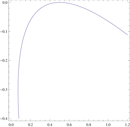
Figure 3: The graph $\Gamma$ of $p^{2}+\left(\frac{1}{2}+\frac{3}{2}U\right)p+\frac{1}{2}\left(U-\frac{1}{2}\right)^{2}=0$ for $U\in\left[0,1.2\right]$ and $p\in\left[-0.4,0\right]$.

The points of $\Gamma$ are evident. If $p$ is considered as a parameter,

$$U=\frac{1}{2}\left(1-3p\pm\sqrt{p^{2}-10p}\right)$$

and if $U$ is considered as a parameter,

$$p=\frac{1}{4}\left(-1-3U\pm\sqrt{U^{2}+14U-1}\right).$$

The solutions of $U^{2}+14U-1=0$ are $U=-7\pm 5\sqrt{2}$ but, as $U$ is a real square $\left(\frac{N}{\pi\rho}\right)^{2}\sin^{2}\left(\frac{\pi s}{N}\right)$, the only admissible value is $U_{c}=-7+5\sqrt{2}\sim 0.071$ and for $U_{c}$ the two values of $p$ are equal to $-\frac{1}{4}\left(1+3U\right)\sim 0.30325$. For $U>U_{c}$, the two $p$ roots are real and for $0\leq U<U_{c}$, they have an imaginary part $\mathop{\mathrm{I}m}\left(p\right)=\pm\sqrt{U^{2}+14U-1}$ while the real part move on the segment $\mathop{\mathrm{R}e}\left(p\right)=-\frac{1}{4}\left(1+3U\right)$ from the point $\left(U=0,p=-\frac{1}{4}\right)$ to the point $\left(U\sim 0.071,p\sim 0.30325\right)$. In what concerns $p$, as $U$ is real, we must have $\sqrt{p^{2}-10p}$ real, that is $p^{2}-10p\geq 0$ i.e. $p\in\left(-\infty,0\right]$ or $p\in\left[10,+\infty\right)$.

The figure 4 reproduces Turing’s figure 1 which displays $\mathop{\mathrm{R}e}\left(p\right)$ and $-\left|\mathop{\mathrm{I}m}\left(p\right)\right|$ as functions of $U$ for $I=0$.

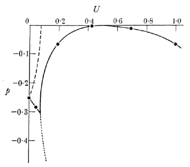
Figure 4: Turing’s figure 1 which displays $\mathop{\mathrm{R}e}\left(p\right)$ and $-\left|\mathop{\mathrm{I}m}\left(p\right)\right|$ as functions of $U$ for $I=0$. The full line and the dotted line represent respectively $\mathop{\mathrm{R}e}\left(p_{s}\right)$ and $\mathop{\mathrm{R}e}\left(p_{s}^{\prime}\right)$, while the broken line represents $-\left|\mathop{\mathrm{I}m}\left(p\right)\right|$. Turing has indicated with black thick points the integer values from $s=0$ (left) to $s=5$ (right).

7 Conditions for instability and the critical point

In the §9 “Further considerations on the mathematics of the ring”, Turing analyzes further the conditions under which a diffusion-driven instability can occur. We will present and complete his computations using the continuous model which is easier to understand.

As reaction-diffusion equations are linear, and since every function on $S^{1}$ is a linear superposition of harmonics $e^{ik\theta}$, we look at solutions of the form

$$\left(\begin{array}[]{c}x\\ y\end{array}\right)=e^{\lambda t}e^{ik\theta}\left(\begin{array}[]{c}x_{0}\\ y_{0}\end{array}\right)$$

which implies immediately

$$\left(\begin{array}[]{c}\dot{x}\\ \dot{y}\end{array}\right)=\lambda e^{\lambda t}e^{ik\theta}\left(\begin{array}[]{c}x_{0}\\ y_{0}\end{array}\right)=$$

$$J_{0}e^{\lambda t}e^{ik\theta}\left(\begin{array}[]{c}x_{0}\\ y_{0}\end{array}\right)+\left(\begin{array}[]{cc}\mu^{\prime}&0\\ 0&\nu^{\prime}\end{array}\right)\left(-k^{2}e^{\lambda t}e^{ik\theta}\right)\left(\begin{array}[]{c}x_{0}\\ y_{0}\end{array}\right),\text{ that is }$$

$$\left(J_{0}-k^{2}D-\lambda I\right)\left(\begin{array}[]{c}x\\ y\end{array}\right)=0,\text{ with }D=\left(\begin{array}[]{cc}\mu^{\prime}&0\\ 0&\nu^{\prime}\end{array}\right)$$

The characteristic equation is therefore

$$\mathop{\mathrm{D}et}\left(J_{0}-k^{2}D-\lambda I\right)=\mathop{\mathrm{D}et}\left(\begin{array}[]{cc}a-\mu^{\prime}k^{2}-\lambda&b\\ c&d-\nu^{\prime}k^{2}-\lambda\end{array}\right)=0$$

and the dispersion relations are

$$\left(\lambda-a+\mu^{\prime}k^{2}\right)\left(\lambda-d+\nu^{\prime}k^{2}\right)=bc$$

or, if we write this equation $\lambda^{2}-S\left(k^{2}\right)\lambda+P\left(k^{2}\right)=0$ with $S\left(k^{2}\right)$ the sum of its two roots and $P\left(k^{2}\right)$ their product,

$$\lambda^{2}-\left(\mathop{\mathrm{T}r}\left(J_{0}\right)-k^{2}\mathop{\mathrm{T}r}\left(D\right)\right)\lambda+\left(\mu^{\prime}\nu^{\prime}k^{4}-\left(\nu^{\prime}a+\mu^{\prime}d\right)k^{2}+\mathop{\mathrm{D}et}\left(J_{0}\right)\right)=0$$

We want $\mathop{\mathrm{T}r}\left(J_{0}\right)=a+d<0$ and $\mathop{\mathrm{D}et}\left(J_{0}\right)=ad-bc>0$ to ensure the stability of the internal chemical equilibrium. But we want also one $\lambda$ with $\mathop{\mathrm{R}e}\left(\lambda\right)>0$ to ensure a diffusion-driven instability. As $\mathop{\mathrm{T}r}\left(J_{0}\right)<0$ and $\mathop{\mathrm{T}r}\left(D\right)=\mu^{\prime}+\nu^{\prime}>0$, this implies $S\left(k^{2}\right)=\mathop{\mathrm{T}r}\left(J_{0}\right)-k^{2}\mathop{\mathrm{T}r}\left(D\right)<0$. If $P\left(k^{2}\right)$ happened to be $>0$, we would have two roots with $\mathop{\mathrm{R}e}\left(\lambda\right)<0$, so we must have $P\left(k^{2}\right)<0$. But as $\mathop{\mathrm{D}et}\left(J_{0}\right)>0$ by hypothesis and of course $\mu^{\prime}\nu^{\prime}k^{4}>0$, we need in fact $\nu^{\prime}a+\mu^{\prime}d>\mu^{\prime}\nu^{\prime}k^{2}+\mathop{\mathrm{D}et}\left(J_{0}\right)/k^{2}>0$. This is a first condition. As $\mathop{\mathrm{T}r}\left(J_{0}\right)=a+d<0$ and $\mu^{\prime},\nu^{\prime}>0$, we need $\mu^{\prime}\neq\nu^{\prime}$ since, if $\mu^{\prime}$ and $\nu^{\prime}$ would be equal, we would have $\nu^{\prime}a+\mu^{\prime}d=\mu^{\prime}\left(a+d\right)<0$.

It is essential to strongly emphasize here the fact that the diffusibility of the two morphogens $X$ and $Y$ must be sufficiently different in order that an instability can occur. It is the key of Turing’s discovery.

In the example of §10, $\mu^{\prime}=\alpha\frac{1}{2}$, $\nu^{\prime}=\alpha\frac{1}{4}$ $\left(\alpha>0\right)$, $a=-2$, $d=\frac{3}{2}$ and the condition $\nu^{\prime}a+\mu^{\prime}d=\alpha\left(-2\times\frac{1}{4}+\frac{3}{2}\times\frac{1}{2}\right)=\frac{\alpha}{4}>0$ is therefore satisfied.

There is a second condition. $P\left(k^{2}\right)=\mu^{\prime}\nu^{\prime}k^{4}-\left(\nu^{\prime}a+\mu^{\prime}d\right)k^{2}+\mathop{\mathrm{D}et}\left(J_{0}\right)$ is a second degree polynomial in $k^{2}$ and we want it to become $<0$ for values of $k^{2}$ which must necessarilly be positive since $k^{2}$ is a real square. Let $\delta=\frac{\mu^{\prime}}{\nu^{\prime}}$. The graph of $P\left(k^{2}\right)$ is a parabola $\Pi$ starting at $\mathop{\mathrm{D}et}\left(J_{0}\right)>0$ for $k=0$. If $\delta<\delta_{c}$ for a critical value to be computed, $\Pi$ is over the $k^{2}$-axis and the condition $P\left(k^{2}\right)<0$ cannot be satisfied. But if $\delta>\delta_{c}$, $\Pi$ intersects the $k^{2}$-axis at two points $k_{1}^{2}$ and $k_{2}^{2}>k_{1}^{2}$ and inside the interval $\left[k_{1}^{2},k_{2}^{2}\right]$ the condition $P\left(k^{2}\right)<0$ is satisfied: there exists an eigenvalue $\lambda$ with $\mathop{\mathrm{R}e}\left(\lambda\right)>0$.

The computation of $\delta_{c}$ is rather tedious. Let $u=k^{2}$. The polynomial $P\left(u\right)$ and its first and second derivatives are

$$P\left(u\right) = \mu^{\prime}\nu^{\prime}u^{2}-\left(\nu^{\prime}a+\mu^{\prime}d\right)u+ad-bc$$

$$P^{\prime}\left(u\right) = -\left(\nu^{\prime}a+\mu^{\prime}d\right)+2\mu^{\prime}\nu^{\prime}u$$

$$P^{\prime\prime}\left(u\right) = 2\mu^{\prime}\nu^{\prime}$$

So the minimum of $\Pi$ is given by $P^{\prime}\left(u\right)=-\left(\nu^{\prime}a+\mu^{\prime}d\right)+2\mu^{\prime}\nu^{\prime}u=0$ and it is a minimum since $P^{\prime\prime}\left(u\right)=2\mu^{\prime}\nu^{\prime}>0$. Its value is

$$u_{0}=k_{0}^{2}=\frac{\nu^{\prime}a+\mu^{\prime}d}{2\mu^{\prime}\nu^{\prime}}$$

and we have

$$P\left(k_{0}^{2}\right)=ad-bc-\frac{1}{4}\frac{\left(\nu^{\prime}a+\mu^{\prime}d\right)^{2}}{\mu^{\prime}\nu^{\prime}}$$

For $P\left(k^{2}\right)$ to become $<0$, we must have therefore

$$0<ad-bc<\frac{1}{4}\frac{\left(\nu^{\prime}a+\mu^{\prime}d\right)^{2}}{\mu^{\prime}\nu^{\prime}}=\frac{1}{4}\frac{\left(a+\delta d\right)^{2}}{\delta}$$

and $\delta_{c}$ is given by the equation

$$ad-bc=\frac{1}{4}\frac{\left(a+\delta_{c}d\right)^{2}}{\delta_{c}}$$

In the example, when $\gamma=0$, we have $ad-bc=\frac{1}{8}$, $\nu^{\prime}a+\mu^{\prime}d=\frac{\alpha}{4}$, $\mu^{\prime}\nu^{\prime}=\frac{\alpha^{2}}{8}$, and we verify that $\frac{1}{8}=\frac{1}{4}\times\left(\frac{1}{4}\right)^{2}\times 8$. So Turing’s system is at its critical point for $\gamma=0$.

Let us now investigate more precisely the second degree equation giving $\delta_{c}$. It can be written

$$d^{2}\delta_{c}^{2}+2\left(2bc-ad\right)\delta_{c}+a^{2}=0$$

and its two solutions are

$$\delta_{c\pm}=\frac{ad-2bc\pm 2\sqrt{-bc\left(ad-bc\right)}}{d^{2}}$$

But as one root, and hence both roots, must be real, we need $-bc\left(ad-bc\right)>0$ and, as $ad-bc>0$ by hypothesis, we must have $bc<0$.

In the example, for $\gamma=0$, we have effectively $-\frac{25}{16}\times 2<0$ and

$$\delta_{c}=\left(\frac{1}{32}\right)^{2}\left[\frac{1}{8}-\left(-\frac{25}{16}\times 2\right)+2\sqrt{\left(\frac{25}{16}\right)\times\left(\frac{1}{8}\right)}\right]=2=\delta$$

As $\delta=\delta_{c}$ we are indeed at the critical point. Then

$$P\left(k^{2}\right)=\frac{\alpha^{2}}{8}k^{4}-\frac{\alpha}{4}k^{2}+\frac{1}{8}=\frac{1}{8}\left(\alpha k^{2}-1\right)^{2}$$

and the parabola $\Pi$ is tangent at the $k^{2}$-axis and at the point of tangency the eigenvalues are $\lambda_{+}=0$ and $\lambda_{\_}=\mathop{\mathrm{T}r}\left(J_{0}\right)-k^{2}\mathop{\mathrm{T}r}\left(D\right)=-\left(\frac{3\alpha}{4}k^{2}\right)-\frac{1}{2}<0$. So, at the crossing of the critical point, the eigenvalue $\lambda_{+}$ becomes $>0$.

8 The bifurcation

After having analyzed the conditions of a diffusion-driven instability at a critical point, Turing analyzed further the behavior of the system in the neighbourhood of the critical point. To this end, he varied the small parameter $\gamma$ around its critical value $\gamma=0$. Today, computations are very easy, but at his time they were difficult and he must use the computer he had himself constructed. We will first do them for the continuous model and then return to Turing’s own discrete model.

8.1 Continuous model

The chemical internal equilibrium is now given by the concentrations of morphogens

$$X_{0}=\frac{1}{7}\left(-25+\sqrt{2^{10}+7\times 55\gamma}\right),~{}Y_{0}=1$$

We linearize the system in the neighbourhood of $\left(X_{0},Y_{0}\right)$ and compute first order expansions in the small parameter $\varepsilon=\frac{7\times 55}{2^{10}}\gamma=\frac{385}{1024}\gamma$. We get

$$a=-2-\varepsilon,b=-\frac{25}{16}-\frac{25}{7}\varepsilon,c=2+\varepsilon,d=\frac{3}{2}+\frac{25}{7}\varepsilon$$

and the conditions for instability: $\mathop{\mathrm{T}r}\left(J_{0}\right)=a+d=-\frac{1}{2}+\frac{18}{7}\varepsilon$ must be $<0$, which implies $\varepsilon<\frac{7}{36}\sim 0.194$; $\nu^{\prime}a+\mu^{\prime}d=\frac{1}{4}+\frac{43}{28}\varepsilon$ must be $>0$, which implies $\varepsilon>-\frac{7}{43}$; $\mathop{\mathrm{D}et}\left(J_{0}\right)=ad-bc=\frac{1}{8}+\frac{1}{16}\varepsilon$ must be $>0$, which implies $\varepsilon>-2$; $ad$ must be $<0$, which implies $\varepsilon>-\frac{42}{121}$; $ad-bc$ must be $<\frac{1}{4}\frac{\left(\nu^{\prime}a+\mu^{\prime}d\right)^{2}}{\mu^{\prime}\nu^{\prime}}$, which implies $\varepsilon>0$.

The equation yielding the eigenvalues is now

$$\lambda^{2}-\left(\mathop{\mathrm{T}r}\left(J_{0}\right)-k^{2}\mathop{\mathrm{T}r}\left(D\right)\right)\lambda+P\left(k^{2}\right)=0$$

Figure 5 displays the graph of $P\left(k^{2}\right)$ for $\varepsilon=0.1.\$The roots of $P\left(k^{2}\right)=0$ are $0.367$ and $2.862$ and inside their interval we have $P\left(k^{2}\right)<0$.

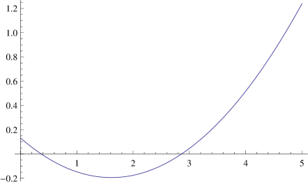
Figure 5: The graph of $P\left(k^{2}\right)$ for $\varepsilon=0.1$. Inside the interval $\left[0.367,2.862\right]$ of $k^{2}$ we have $P\left(k^{2}\right)<0$.

The characteristic equation is

$$\lambda^{2}-\left(\mathop{\mathrm{T}r}\left(J_{0}\right)-k^{2}\mathop{\mathrm{T}r}\left(D\right)\right)\lambda+\left(\mu^{\prime}\nu^{\prime}k^{4}-\left(\nu^{\prime}a+\mu^{\prime}d\right)k^{2}+\mathop{\mathrm{D}et}\left(J_{0}\right)\right)=0$$

that is

$$\lambda^{2}+\left(\frac{1}{2}+\frac{3k^{2}}{4}-\frac{18}{7}\varepsilon\right)\lambda+\left(\frac{k^{4}}{8}-\left(\frac{1}{4}+\frac{43}{28}\varepsilon\right)k^{2}+\frac{1}{8}+\frac{1}{16}\varepsilon\right)=0$$

and its roots $\lambda_{\pm}$ are approximated by

$$\frac{1}{128}\left(-7+36\varepsilon\pm\sqrt{-49-553\varepsilon+1296\varepsilon^{2}+490k^{2}-308\varepsilon k^{2}+343k^{4}}\right)$$

Figures 7 and 9 display the graphs of $\lambda_{+}$ and $\lambda_{\_}$ (including the irrelevant negative $k^{2}$-axis). For $\lambda_{+}$ we see that $\lambda_{+}\geq 0$ for $k^{2}\in\left[0.367,2.862\right]$. Figure 8 zooms on this interval. There is no graph inside the open interval $\left]-1.5146,0.1758\right[$ where the discriminant $\Delta$ of the characteristic equation is $<0$ (see figure 6).

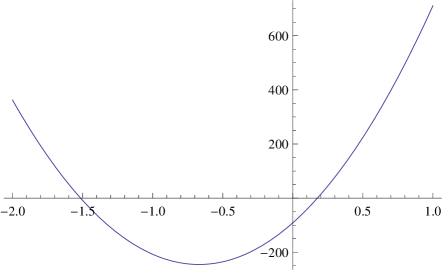
Figure 6: The discriminant $\Delta\left(k^{2}\right)$ for $\varepsilon=0.1$. $\Delta$ is negative inside the open interval $\left]-1.5146,0.1758\right[.$

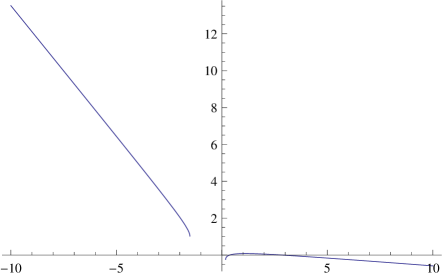
Figure 7: Graph of $\lambda_{+}$ (including the irrelevant negative $k^{2}$-axis). $\lambda_{+}\geq 0$ for $k^{2}\in\left[0.367,2.862\right]$. There is no graph inside the open interval $\left]-1.5146,0.1758\right[$ where the discriminant $\Delta$ of the characteristic equation is $<0$.

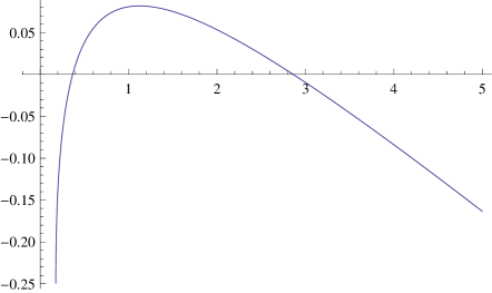
Figure 8: Zoom on the interval $k^{2}\in\left[0.367,2.862\right]$ of the figure 7 where $\lambda_{+}\geq 0$.

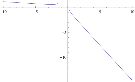
Figure 9: Graph of $\lambda_{\_}$ (including the irrelevant negative $k^{2}$-axis). $\lambda_{\_}\$is always $<0$ for $k^{2}>0$. There is no graph inside the open interval $\left]-1.5146,0.1758\right[$ where the discriminant $\Delta$ of the characteristic equation is $<0$.

8.2 Discrete model

Let us come back to the discrete ring model composed of $N=20$ cells. At the critical point $\gamma=0$, the $20$ characteristic equations in the Fourier domain are

$$\left(p+2+2\sin^{2}\left(\frac{\pi s}{20}\right)\right)\left(p-1.5+\sin^{2}\left(\frac{\pi s}{20}\right)\right)+\frac{25}{8}=0$$

The figure 10 shows the table of the $20$ pairs $\left(p_{s},p_{s}^{\prime}\right)$ of eigenvalues for $s=0,\ldots,19$. We see that if we order the $p$ w.r.t to increasing $\mathop{\mathrm{R}e}\left(p\right)$ we get $p_{3}=p_{17}=-0.00346$, $p_{4}=p_{16}=-0.012$, $p_{5}=p_{15}=-0.064$, $p_{2}=p_{18}=-0.066$. It is therefore the mode $p_{3}$ which can most readily become $>0.$

Figure 10: The table of the $20$ pairs $\left(p_{s},p_{s}^{\prime}\right)$ of eigenvalues of the discrete ring model for $s=0,\ldots,19$ and $\gamma=0$.

Let us now vary the small slow parameter $\gamma.$ Turing varied $\gamma$ almost adiabatically from $-\frac{1}{4}$ (stability) to $\frac{1}{16}$ (instability) at speed $\dot{\gamma}=2^{-7}=\frac{1}{128}$. This corresponds to variations $\varepsilon:-0.094\rightarrow 0.0235$ for $\varepsilon$ and $t:0\rightarrow 40$ for the discrete time $t$. For $\gamma=-\frac{1}{4}$, the equilibrium is $\left(X_{0}=0.78,Y_{0}=1\right)$, and $a_{0}=-1.9$, $b_{0}=-1.218$, $c_{0}=1.9$, $d_{0}=1.156$, and all $\mathop{\mathrm{R}e}\left(p_{s}\right)<0$: the system is stable. On the contrary, for $\gamma=-\frac{1}{16}$, the equilibrium is $\left(X_{1}=1.053,Y_{1}=1\right)$, and $a_{1}=-2.023$, $b_{1}=-1.646$, $c_{1}=2.023$, $d_{1}=1.583$, and $p_{3}=p_{17}=0.0224>0$, $p_{4}=p_{16}=0.012>0$: the system is unstable. The figure 11 shows the table of the $20$ pairs $\left(p_{s},p_{s}^{\prime}\right)$ of eigenvalues for $s=0,\ldots,19$ for $\gamma=\frac{1}{16}$.

Figure 11: The table of the $20$ pairs $\left(p_{s},p_{s}^{\prime}\right)$ of eigenvalues of the discrete ring model for $s=0,\ldots,19$ and $\gamma=\frac{1}{16}$.

In figure 12 we show the $20$ graphs $\mathop{\mathrm{R}e}\left(p_{s}\right)$ as functions of $t$ for $\gamma$ varying from $-\frac{1}{4}$ to $\frac{1}{16}$. The time $t$ varies from $t=0$ to $t=40$. We see the $\mathop{\mathrm{R}e}\left(p_{s}\right)$ which become $>0$ for $s=3,17,4,16$. At $t=40$, $p_{3}=p_{17}=0.0224$ and $p_{4}=p_{16}=0.012$. For $s=0,1,19$, $\mathop{\mathrm{R}e}\left(p_{s}\right)$ presents an angular point because $p_{s}$ is a complex number with $\mathop{\mathrm{I}m}\left(p_{s}\right)\neq 0$. It is the same phenomenon as in the toy model of figure 4. Figure 13 shows the graphs of $\mathop{\mathrm{R}e}\left(p\right)$ and $\mathop{\mathrm{I}m}\left(p\right)$ in such a case.

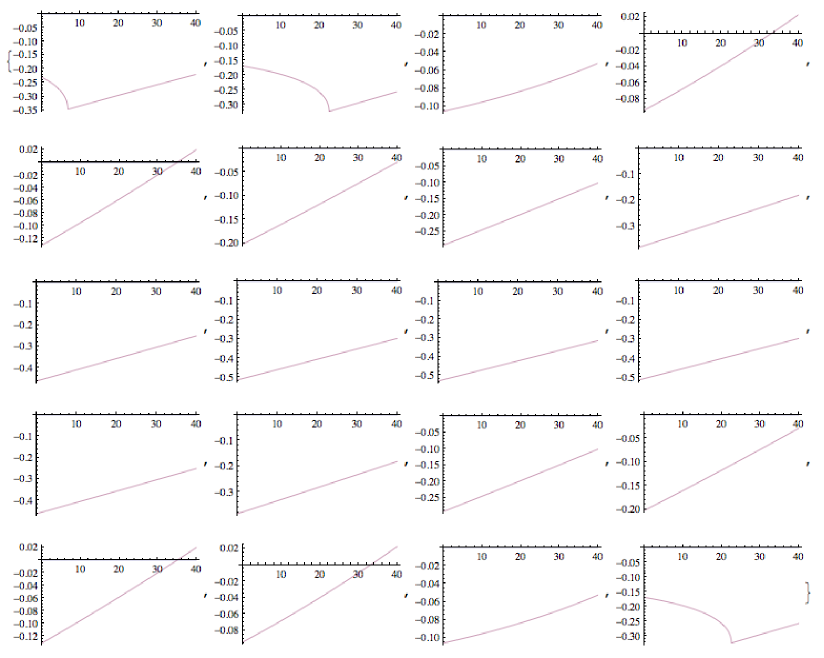
Figure 12: The $20$ graphs $\mathop{\mathrm{R}e}\left(p_{s}\right)$ as functions of $t$ for $\gamma$ varying from $-\frac{1}{4}$ to $\frac{1}{16}$. The time $t$ varies from $t=0$ to $t=40$. The $\mathop{\mathrm{R}e}\left(p_{s}\right)$ become $>0$ for $s=3,17,4,16$. At $t=40$, $p_{3}=p_{17}=0.0224$ and $p_{4}=p_{16}=0.012$. For $s=0,1,19$, $\mathop{\mathrm{R}e}\left(p_{s}\right)$ presents an angular point because $p_{s}$ is a complex number with $\mathop{\mathrm{I}m}\left(p_{s}\right)\neq 0$. It is the same phenomenon as in the toy model of figure 4.

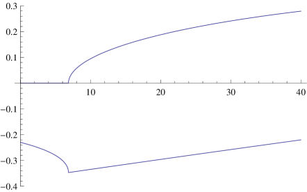
Figure 13: When $\mathop{\mathrm{I}m}\left(p\right)\neq 0$ (graph up), $\mathop{\mathrm{R}e}\left(p\right)$ (graph down) presents an angular point.

In his paper, Turing computes (with his recently constructed Manchester computer) the table of the evolution of the ring (see figure 14) and shows how Fourier modes become dominant after the bifurcation induced by the diffusion-driven instability (see figure 15). In the initial state, all cells are, up to small fluctuations, in the equilibrium state $\left(X_{0}=1,Y_{0}=1\right)$. After the bifurcation, a stationary oscillatory wave pattern with $3$ lobes develops. The divergences induced by the instability are tamed by two factors: (i) the concentration $X$ cannot become $<0$ and when $X\left(r,t\right)$ vanishes, the process stops locally, (ii) saturation non-linear effects allow a new equilibrium to occur. These results constitute a great achievement.

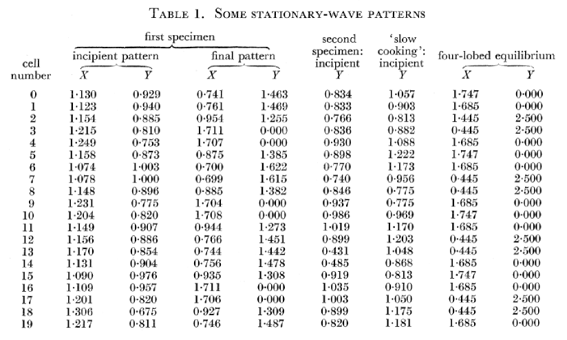
Figure 14: Turing’s computation of the evolution of the ring.

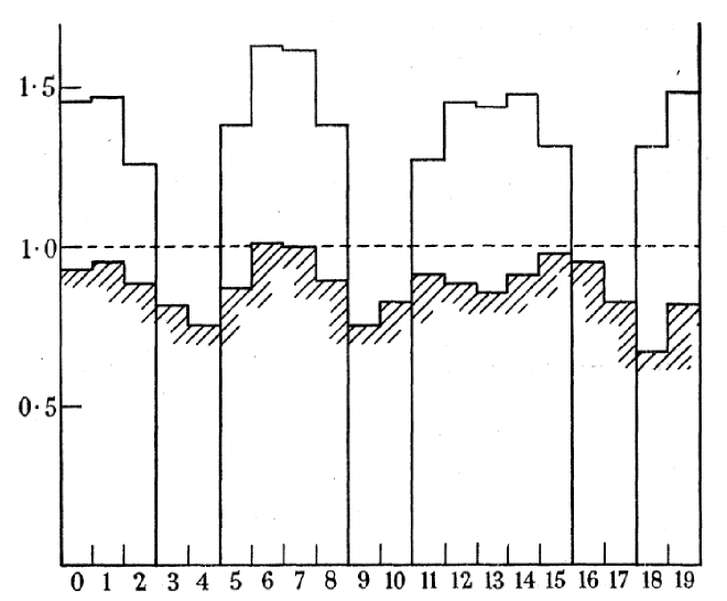
Figure 15: The evolution of the ring after the bifurcation induced by a diffusion-driven instability. The hatched graph represents the $X$ concentration at the initial state: all cells are, up to small fluctuations, in the equilibrium state $\left(X_{0}=1,Y_{0}=1\right)$. The other graph represents a stationary oscillatory wave pattern with $3$ lobes. The divergences induced by the stability are tamed by two factors: (i) the concentration $X$ cannot become $<0$, (ii) non-linear effects.

9 Further aspects of Turing’s paper

In his paper, Turing evoked many other problems. In §4 he gave simple examples for explaining the idea of “breakdown of symmetry and homogeneity” in pattern formation. He explained also how exponential divergences are bounded by non-linearities which allow new equilibria to emerge and he emphasized

“the effect of considering non-linear reaction rate functions when far from homogeneity.” (p. 58)

In §8 he listed some “types of asymptotic behaviours in the ring after a lapse of time”:

1. “stationary cases” where the asymptotic regime is dominated by a pair of real eigenvalues $\left(p_{s_{0}},p_{s_{0}}^{\prime}\right)$;

2. “oscillatory cases” where the asymptotic regime is dominated by a pair of complex conjugated eigenvalues $\left(p_{s_{0}},p_{s_{0}}^{\prime}\right)$ (travelling waves);

3. “limit cases”.

He drew also phase diagrams in the parameter space which classify these different regimes and explained the role of fluctuations in the bifurcation process.

Another extremely important anticipation is that in two-dimensionsional tissues diffusion-driven instabilities can explain “dappled colour patterns” as observed on sea shells or leopard’s coats. Figure 16 reproduces Turing’s figure 2.

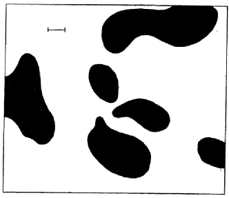
Figure 16: Turing’s figure 2 on “dappled colour patterns” in two-dimensionsional tissues.

Moreover, Turing anticipated the fact that his general model was able to induce oscillating patterns when the chemical internal dynamics of each cell bifurcates towards a limit cycle by Hopf bifurcation. When such limit cycles propagate spatially, many complex phenomena can emerge. Turing envisaged applications to organisms such as plants (flowers, leaves) or Hydra. His predictions have been widely confirmed later.

In the fascinating §12 “Chemical waves on spheres. Gastrulation”, Turing generalizes his one-dimensional ring model to a two-dimensional sphere model whose geometry is more complex, the harmonic analysis on the sphere resting on the eigenfunctions of the spherical Laplacian, namely the spherical harmonics. His striking idea was to apply the model to gastrulation in embryology, which is the step at which the spherical symmetry of the blastula is broken. He developed this idea further in his unpublished paper on phyllotaxis.

Finally, in the last §13 “Non-linear theory. Use of digital computer”, Turing came back to the assumption that linearization is a good approximation and explained that it is the case only in the neighbourhood of the first bifurcation. It is

“an assumption which is justifiable in the case of a system just beginning to leave a homogeneous condition.” (p. 72)

For Turing it was risky to try to go beyond:

“One cannot hope to have any very embracing theory of such processes, beyond the statement of the equations.” (p. 73)

Hence the fundamental interest of the just constructed digital computers enabling numerical simulations avoiding the too drastic simplifications imposed by the search of explicit theoretical solutions to the equations.

10 Conclusion: after Turing

To conclude this presentation of Turing’s 1952 paper, let us look briefly at the works on reaction-diffusion equations after Turing. I have already tackle this theme in my talk [19] at the IAPS 2001 Conference on Complexity and Emergence.

10.1 General reaction-diffusion models

Among the many specialists of the domain, we would cite Hans Meinhardt and Alfred Gierer who, since 1972 [5], have considerably increased our knowledge on reaction-diffusion models. They have shown that, for an activator/inhibitor pair of morphogens, instabilities mainly result from the competition between a short range slow activation and a long range fast inhibition, the inhibitor diffusing faster than the excitator. This confirms Turing’s remark on the role of the difference between the two diffusibility coefficients $\mu$ and $\nu$.

A general Meinhardt-Gierer model has the form

$$\left\{\begin{array}[]{l}\dot{x}=\rho\frac{x^{2}}{y}-\alpha x+\sigma_{x}+\mu\Delta x\\ \dot{y}=\rho x^{2}-\beta y+\sigma_{y}+\nu\Delta y\end{array}\right.~{}\alpha<\beta,~{}\mu\ll\nu$$

The activator morphogen $x$ is self-catalizing ($x^{2}$ term in $\dot{x}$) and its production is inhibited by the inhibitor morphogen $y$ ($\frac{1}{y}$ term in $\dot{x}$). Moreover, $x$ catalyzes its inhibitor ($x^{2}$ term in $\dot{y}$). The linear terms $\alpha x$ and $\beta y$ ($\alpha<\beta$) are degradation terms, the constant $\sigma_{y}$ enables a stable homogeneous state and the constant $\sigma_{x}$ allows to trigger the process. $\mu$ and $\nu$ are the diffusibility coefficients with $\mu$ (slow)$~{}\ll\nu$ (fast). A local fluctuation of the activator $x$ induces a local peak of $x$ which diffuses slowly. But it amplifies also the inhibitor concentration $y$, and since $y$ diffuses faster than $x$ it will inhibit the production of $x$ at some distance (what is called a “lateral inhibition”).

The coupling between the internal dynamics and external diffusion can induce very complex patterns. Figure 17 shows two examples due to De Kepper [3], a system of stripes with defects and a honeycomb pattern.

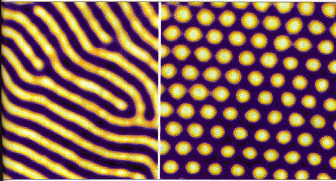
Figure 17: The coupling between internal dynamics and external diffusion can induce very complex patterns. Two examples due to De Kepper: a system of stripes (with defects) and a honeycomb pattern. (From De Kepper et al. [3]).

One of the best known achievements of Hans Meinhardt is his modelling of sea shells. Since the growth of a shell results from an accretion of calcified matter along its boundary, it can be represented by a two-dimensional diagram $B\times T=$ boundary$\times$time. The geometry is therefore in fact one-dimensional. The diffusion of the activator from a local peak of concentration induces a triangle where the pigmentation controlled by $x$ is high, but the faster diffusion of the inhibitor stops it after a while. Hence a cascade of triangles. Figure 18 shows the celebrated model of Conus marmoreous.

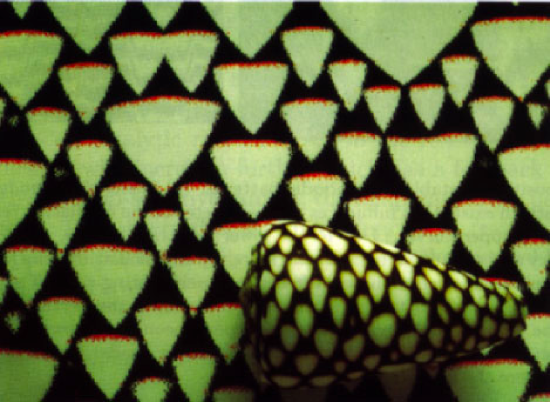
Figure 18: Meinhardt’s model for the sea shell Conus marmoreous. In front a true shell. In the background its reaction-diffusion model. (From Meinhardt [10]).

10.2 From Alan Turing to René Thom

As we have seen, in Turing’s paper morphogenetic processes spatially unfold diffusion-driven instabilities. In the late 1960s, René Thom [20], [21] proposed a more general model based on the general concept of bifurcation. The similarities and dissimilarities between Turing’s and Thom’s models are fascinating. The key idea is the same: internal chimical dynamics (reactions) are coupled with external spatial dynamics, the latter destabilize the former and morphologies spatially unfold the instabilities. As we have seen, in Turing coupling is given by the diffusion of the reacting morphogens. In Thom, coupling is more generally a spatial control of internal dynamics and the morphogenetic discontinuities breaking the homogeneity of the substrate are induced by bifurcations.

10.3 Beyond Turing

After Turing, many authors, e.g. James Murray [14], [15], introduced bifurcations in reaction-diffusion equations. Let $u$ be the vector $\left(x,y\right)$ and consider a differential equation $\dot{u}=f\left(u,r\right)$ where $r$ is a spatial control. When $r$ varies and crosses a critical value $r_{c}$, the initial stable equilibrium state $u_{0}$ of the system can collapse with an unstable equilibrium and disappear. The system is therefore projected to another equilibrium through this saddle-node bifurcation. Another most used bifurcation is the Hopf bifurcation. When $r$ varies and crosses a critical value $r_{c}$, the initial stable (i.e. attracting) equilibrium state $u_{0}$ becomes a repellor and generates a small attracting closed orbit (i.e. a limit cycle).

Consider for instance the following system analyzed by Robin Engelhardt [4]:

$$\left\{\begin{array}[]{l}\dot{x}=-xy^{2}+ay-\left(1+b\right)x+\delta\Delta x\\ \dot{y}=xy^{2}-\left(1+a\right)y+x+F+\delta\Delta y\end{array}\right.$$

The chemical internal equilibria without diffusion ($\delta=0$) are solutions of the equations (if $y^{2}+1+b\neq 0$):

$$x=\frac{ay}{y^{2}+1+b}$$

$$a\frac{y^{3}}{y^{2}+1+b}-\left(1+a\right)y+\frac{ay}{y^{2}+1+b}+F=0$$

that is

$$y^{3}-Fy^{2}+\left(1+b+ab\right)y-F\left(1+b\right)=0$$

which is a cubic equation with parameters $a,b,F$.

At the points where $y^{2}+1+b=0$, we have

$$\left\{\begin{array}[]{l}\dot{x}=ay+\delta\Delta x\\ \dot{y}=-bx-\left(1+a\right)y+F+\delta\Delta y\end{array}\right.$$

and this can be an equilibrium point for $\delta=0$ only if $ay=0$ and $-bx-y+F=0$. If $a\neq 0$, this implies the condition $b=-1$, and the equilibrium is $y=0$, $x=-F$. If $a=0$, the equilibrium would be $-bx-y+F=0$ with $y^{2}+1+b=0$. Figure 19 shows some examples of patterns solution of this system of equations.

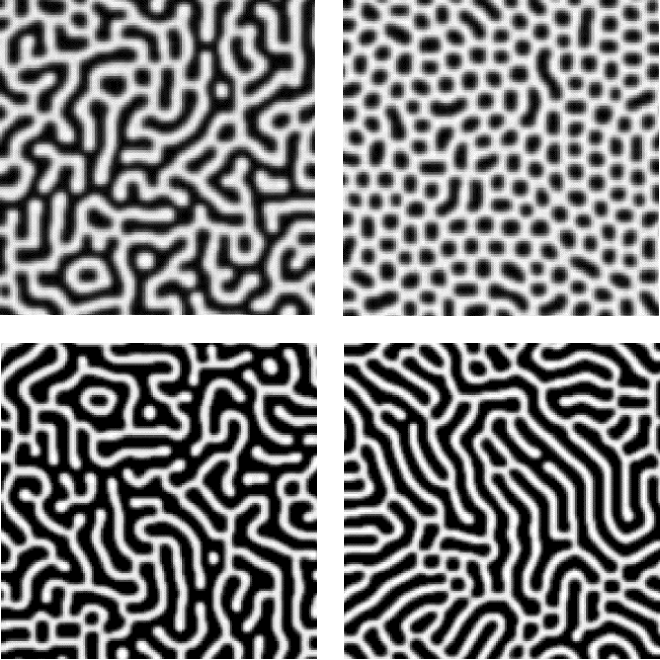
Figure 19: Some examples of patternized solutions of Engelhardt’s system of equations. (From [4]).

There is a wealth of material on these topics. The reader could look e.g. at Harrison [6], Lee et al. [7], [8], Maini [9], Oyang-Swinney [16], or Pearson [17].

10.4 Experimental results

The validity of Turing’s models for embryology are still under discussion. But in what concerns chimical and biological patterns their validity is without doubt. We have seen Meinhardt’s examples. For chemical systems exact verifications go back to 1990 and the works of the Bordeaux group of Patrick De Kepper (Castets, Dulos, Boissonade) on iodate-ferrocyanide-sulfite or clorite-iodide-malonic acid-starch reactions in gel reactors.

It is a full universe of morphological phenomena and mathematical models that Turing opened in 1952 with a remarkable foresightedness.

References

- [1] D’Arcy Thompson, 1942. On Growth and Form, Cambridge University Press, Cambridge.
- [2] V. Castets, E. Dulos, J. Boissonade, P. De Kepper, 1990. “Experimental evidence of a sustained standing Turing type non-equilibrium chemical pattern”, Physical Review Letter, 64 (1990) 2953-2955.
- [3] P. De Kepper et al. 1998. “Taches, rayures et labyrinthes”, La Recherche, 305, 84-89.
- [4] R. Engelhardt, 1994. Modelling Pattern Formation in Reaction-Diffusion Systems, Thesis, University of Copenhagen.
- [5] A. Gierer, H. Meinhardt, 1972. “A theory of biological pattern formation”, Kybernetik, 12 (1972) 30-39.
- [6] L.G. Harrison, 1987.“What is the status of reaction-diffusion theory thirty-four years after Turing?”, Journal of Theoretical Biology, 125 (1987) 369-384.
- [7] K.J. Lee, W.D. McCormick, Q. Ouyang, H.L. Swinney, 1993. “Pattern Formation by Interacting Chemical Fronts”, Science, 261 (1993) 192-194.
- [8] K.J. Lee, W.D. McCormick, J.E. Pearson, H.L. Swinney, 1994. “Experimental Observation of Self-replicating Spots in a Reaction-diffusion System”, Nature, 369 (1994) 215-218.
- [9] P. Maini, 2012. “Turing’s mathematical theory of morphogenesis, Asia Pacific Mathematics Newsletter, 2, 1 (2012) 7-8.
- [10] H. Meinhardt, 1982. Models of Biological Pattern Formation, Academic Press, London.
- [11] H. Meinhardt, P. Prusinkiewicz, D. Fowler, 2003. The Algorithmic Beauty of Sea Shells, Springer, Berlin, 2003.
- [12] H. Meinhardt, 2012. “Turing’s theory of morphogenesis of 1952 and the subsequent discovery of the crucial role of local self-enhancement and long-range inhibition, Interface Focus, 2, 4 (2012) 407-416.
- [13] L. Michaelis, M. Menthen, 1913. “Die Kinetic der Invertinwirkung”, Biochemische Zeitschrift, 49 (1913) 333-369. Engl. transl. R.S. Goody, K.A. Johnson, “The Kinetics of Invertase Action”, http://path.upmc.edu/divisions/chp/PDF/Michaelis-Menten_Kinetik.pdf.
- [14] J.D. Murray, 1989. Mathematical Biology. An Introduction, Springer, Berlin.
- [15] J.D. Murray, 1990. “Turing’s theory of morphogenesis. Its influence on modelling biological pattern and form”, Bulletin of Mathematical Biology, 52, 1/2 (1990) 119-152.
- [16] Q. Oyang, H.L. Swinney, 1991. “Transition from a uniform state to hexagonal and striped Turing patterns”, Nature, 352 (1991) 610-612.
- [17] J.E. Pearson, 1993. “Complex Patterns in a Simple System”, Science, 261 (1993) 189-192.
- [18] J. Petitot, 2003. Morphogenesis of Meaning, Peter Lang, Bern.
- [19] J. Petitot, 2003. “Modèles de structures émergentes dans les systèmes complexes”, Complexity and Emergence (E. Agazzi, L. Montecucco eds), Proceedings of the Annual Meeting of the International Academy of the Philosophy of Science, World Scientific, Singapore, 57-71.
- [20] R. Thom, 1972. Stabilité structurelle et morphogenèse, Interéditions, Paris.
- [21] R. Thom, 1974. Modèles mathématiques de la morphogenèse, Collection 10/18, Union Générale d’Éditions, Paris.
- [22] A.M. Turing, 1952. “The Chemical Basis of Morphogenesis”, Philosophical Transactions of the Royal Society of London, Series B, Biological Sciences, 237, 641(1952) 37-72.
- [23] A.M. Turing, 1953. “Morphogen Theory of Phyllotaxis”, King’s College Archive Center, Cambrige (unpublished).
- [24] A.M. Turing, C.W. Wardlaw, 1952. “A diffusion reaction theory of morphogenesis in plants”, New Phyt. 52, 40-47. Also in Collected Works of A.M. Turing, P.T. Saunders, Amsterdam, 1953, 37-47.
- [25] C.H. Waddington, 1940. Organizers and Genes, Cambridge University Press, Cambridge.