Dark Matter From Spacetime Nonlocality
Abstract
We propose that dark matter is not yet another new particle in nature, but that it is a remnant of quantum gravitational effects on known fields. We arrive at this possibility in an indirect and surprising manner: by considering retarded, nonlocal, and Lorentzian evolution for quantum fields. This is inspired by recent developments in causal set theory, where such an evolution shows up as the continuum limit of scalar field propagation on a background causal set. Concretely, we study the quantum theory of a massless scalar field whose evolution is given not by the the d’Alembertian , but by an operator which is Lorentz invariant, reduces to at low energies, and defines an explicitly retarded evolution: only depends on , with is in the causal past of . This modification results in the existence of a continuum of massive particles, in addition to the usual massless ones, in the free theory. When interactions are introduced, these massive or off-shell quanta can be produced by the scattering of massless particles, but once produced, they no longer interact, which makes them a natural candidate for dark matter.
I Introduction
The nature of dark matter is one of the most important problems in modern physics. Almost a century after it was hypothesized, though, our understanding of it is still limited to its gravitational signature on luminous matter. It is often assumed that dark matter is a new weakly interacting particle which is just hard to detect. However, so far there has been no conclusive direct or indirect detection in accelerators or cosmological/astrophysical settings. In what follows, we propose that dark matter is not yet another new particle in nature, but that it is a remnant of quantum gravitational effects on known fields. We arrive at this possibility in an indirect and surprising manner: by considering retarded, nonlocal, and Lorentzian evolution for quantum fields. Concretely, we study the consequences of replacing the d’Alembertian with an operator which is Lorentz invariant, reduces to at low energies, and defines a retarded evolution: only depends on , with is in the causal past of . Why is this type of evolution interesting, what does it have to do with quantum gravity, and how does it lead to a proposal for the nature of dark matter?
The causal set theory approach to quantum gravity postulates that the fundamental structure of spacetime is that of a locally finite and partially ordered set Bombelli et al. (1987). Its marriage of discreteness with causal order implies that physics cannot remain local at all scales. This nonlocality manifests itself concretely, for instance, when one seeks to describe the wave propagation of a scalar field on a causal set. It has been shown in this case that coarse-graining the quantum gravitational degrees of freedom leads to a nonlocal field theory described by an operator exactly of the type Sorkin (2007); Aslanbeigi et al. (2014); Benincasa and Dowker (2010); Dowker and Glaser (2013); Glaser (2014). There are reasons to suspect that this type of nonlocality is not necessarily confined to the Planck scale, and that it may have nontrivial implications for physics at energy scales accessible by current experiments (see Woodard (2014); Deser and Woodard (2007) and references therein for implications of nonlocality in the context of cosmology). It is then only natural to wonder what a quantum field theory built upon would look like, especially that it may contain information about the fundamental structure of spacetime.
Studying is also interesting from a purely field-theoretic perspective, since it forces us to relax one of the core assumptions of quantum field theory: locality. Most nonlocal and Lorentzian quantum field theories studied in the literature consider modifications of the type . In this paper, we consider explicitly retarded operators, which are more generic and have more interesting properties as a result. For instance, the Fourier transform of is generically complex, which is a direct consequence of retarded evolution. In fact, this feature is at the heart of our proposal for the nature of dark matter. It is also worth mentioning that quantizing a field theory of the type described here is non-trivial due to the absence of a local action principle. This presents a technical challenge, from which one may gain deeper insight into quantization schemes.
What is the relation between a quantum field theory based on and dark matter? Upon quantizing a free massless scalar field with the classical equation of motion , we find off-shell modes in the mode expansion of the quantized field operator . These are modes which do not satisfy any dispersion relation, unlike in usual local quantum field theory (LQFT) where every Fourier mode with four-momentum is an on-shell quanta, i.e. it satisfies .111 We use a signature of for the Minkowski metric . Also, This is equivalent to the statement that the quantized field operator does not generically satisfy the classical equation of motion: . Note that an off-shell mode of a massless scalar field has an effective mass, and can be thought of as a massive quanta in itself. We show that the off-shell modes can exist in “in” and “out” states of scattering, and are different from virtual particles which exist as intermediate states in Feynman diagrams. When considering the interacting theory, we find an extremely surprising result: the cross-section of any scattering process which contains one or more off-shell particle(s)222In the quantum theory, an off-shell particle is 1-particle quantum state with a well-defined (non-zero) mass and momentum, i.e. a massive eigenstate of Hamiltonian and momentum operator. in the “in” state is zero. That is to say, on-shell quanta can scatter and produce off-shell particles, but once produced, off-shell particles no longer interact. It is this behaviour that makes these off-shell particles a natural candidate for dark matter. The phenomenological story would be that dark matter particles were produced in the early universe in this fashion: as off-shell modes of quantum fields. This feature of the theory can be traced back to the fact that defines an explicitly retarded evolution, which as mentioned previously, may be a remnant of quantum gravitational degrees of freedom.
Our paper is organized as follows. In Section II, we start by setting forth a series of axioms which any non-local, retarded, and Lorentzian modification of at high energies should satisfy. In Section III, we argue there is no action principle for the theory of interest, which forces us to carefully study, in Section IV, what quantization scheme should be used. There, we argue that canonical quantization and the Feynman path-integral approach do not work, and explain why the Schwinger-Keldysh (also known as the double path integral or in-in) formalism provides the appropriate framework. Sections V and VI describe the interacting theory, where we work out the modified Feynman rules, find S-matrix amplitudes, and compute cross-sections for various examples and comment on the time reversibility of the theory. Although a continuum superposition of off-shell particles can in principle scatter into on-shell modes, we argue why this is unlikely to happen. Extension to massive scalar fields is discussed in VII. Section VIII concludes the paper.
II Modified d’Alembertian: Definition
In this section we study generic spectral properties of non-local and Lorentzian modifications of the d’Alembertian . We focus on a class of operators which defines an explicitly retarded evolution: depends only on with in the causal past of . As we will see, such operators have interesting features which are absent in modifications of the type . We start by setting forth a series of axioms which a non-local, retarded, and Lorentzian modification of at high energies should satisfy:
-
1.
Linearity:
(1) where and are complex scalar fields and denotes the set of complex numbers.
-
2.
Reality: for any real scalar field , is also real. Note that reality and linearity imply for any complex scalar field that
(2) where denotes complex conjugation.
-
3.
Poincare-invariance: evolution defined by is Poincare-invariant. Consider a scalar field which transforms to under a Poincare transformation . We require to be invariant under the action of :
(3) Taking to be a spacetime translation , one finds that the eigenfunctions of are plane waves. To see this, let and define . It then follows from (3) that
(4) where we have used the linearity condition. Solutions to the above equation are plane waves:
(5) where is any function of the wave-vector . Therefore, it follows from translational invariance that is an eigenfunction of with the corresponding eigenvalue . Taking to be a Lorentz transformation, it can be shown that can only depend on the the Lorentzian norm of , i.e. , and whether or not is future or past directed, i.e. :
(6) Combining (5) and (2) we find , which using (6) is equivalent to
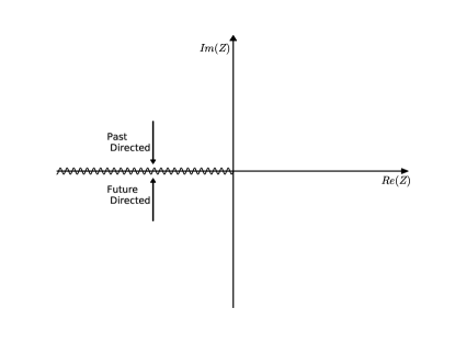
(7) For a spacelike wave-vector , it is always possible to find a coordinate system in which . As a result, is real for spacelike . For timelike momenta, however, may be complex and its imaginary part changes sign when .
Most nonlocal modifications of considered in the literature are of the form , in which case is only a function of . In this paper we focus on a class of nonlocal operators for which does depend on , and find many interesting consequences as a result.
-
4.
Locality at low energies: since provides a good description of nature at low energies, we require in this regime. In other words, expanding for “small” values of , we require the leading order behaviour to be that of :
(8) Note that by a “small” value of , we mean in comparison to a scale which can be interpreted as the non-locality scale, implicitly defined through .
-
5.
Stability: we require that evolution defined by is stable. This condition implies that , when analytically continued to the complex plane of , only has a zero at Aslanbeigi et al. (2014).
-
6.
Retardedness: only depends on , with is in the causal past of .
Let us briefly consider a class of operators which satisfy all the aforementioned axioms. We shall let denote the nonlocality energy scale and define
| (9) |
where is a dimensionless real number, denotes the causal past of , and is the Lorentzian distance between and :
| (10) |
Examples of such operators have arisen in the causal set theory program Sorkin (2007); Aslanbeigi et al. (2014); Benincasa and Dowker (2010); Dowker and Glaser (2013); Glaser (2014). This operator is clearly linear, real, Poincare-invariant and retarded. It is shown in Appendix A that there are choices of and for which is also stable and has the desired infrared behaviour (8). One such choice is
| (11) |
where is an infinitesimally small positive number.
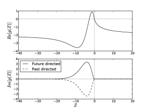
The eigenvalues of take the form (see Aslanbeigi et al. (2014))
| (12) | ||||
| (13) |
where is an infinitesimally small (), timelike, and future-directed () wave-vector. The analytic structure of is shown in Figure 1. Figure 2 shows the behaviour of as a function of and for the choice of and given in (11).
III Classical Theory
How would such non-local and retarded evolution manifest itself? To get a start on answering this question, we modify the evolution of a massless scalar field coupled to a source via :
| (14) |
It is worth noting that the solutions of are identical to those of . This follows from requiring a stable evolution for (see Aslanbeigi et al. (2014)). As we will see in Section III.2, however, the story changes when .
III.1 Absence of an action principle
It is natural to ask whether an action principle exists for , whose variation would produce the non-local equation of motion . One might propose to substitute with in the action of a massless scalar field:
| (15) |
Requiring to be stationary with respect to first order variations in we find 333 To see this, it is instructive to express the action in Fourier space. Define the Fourier transform of via (16) Then, it can be shown that (17) Requiring to be stationary with respect to first order variations we find (18)
| (19) |
where is defined in Fourier space via
| (20) |
In the case of the retarded operator (9), for instance, is the right hand side of (9) with the domain of integration changed to the causal future of point . Therefore, (15) does not lead to a retarded equation of motion.
Due to the absence of a local Lagrangian description, quantizing a massless scalar field theory built upon is non-trivial. We shall address this problem in Section IV, where we argue that the the Schwinger-Keldysh quantization scheme can still be used to obtain the desired non-local quantum field theory.
III.2 Green’s function
The Green’s functions of and are quite different, especially in the ultraviolet (UV) where their spectra differ. One important difference is that , unlike , has a unique inverse. Since is a retarded operator by definition, it only has a retarded Green’s function. Recall that has both a retarded and advanced Green’s function:
| (21) |
which satisfy the following “boundary conditions”: vanishes unless ( is in the causal future of ), and vanishes unless . The two Green’s functions are related to one another via . In the case of , Green’s function is unique (just the retarded one) and switching the arguments of the retarded Green’s function does not produce another Green’s function. Let us show why this is.
Let denote the Green’s function associated with :
| (22) |
Note that can be expressed as
| (23) |
The path of integration in the complex plane is shown in Figure 3. This comes from the fact that is a retarded operator, so analytically continued to the complex plane takes its value above the cut. When has no zeros in complex plane apart from at , which is guaranteed by the stability requirement, this choice of contour ensures that is indeed retarded. Switching the arguments of , we find
| (24) | ||||
| (25) | ||||
| (26) |
where in the second line we have changed integration variables from to . Then
| (27) |
since is generically complex. As we will see in the sections to come, the fact that has a unique inverse plays a crucial role in the quantum theory of .
IV Quantum Theory
We wish to construct a quantum theory of a massless scalar field whose classical limit reproduces the retarded evolution induced by . The quantization scheme which we believe is most suited in this case is the Schwinger-Keldysh (or double path integral) formalism. In what follows, we will first review the usual paths to quantization (i.e. canonical quantization and the Feynman path integral) and show why they fail in the case of a non-local and retarded operator like . The goal of these discussions is to make clear why we choose the Schwinger-Keldysh formalism to construct a quantum field theory based on .
IV.1 Canonical quantization
Let us consider the canonical quantization of a free massless scalar field . The typical route to quantization is as follows: start from an action principal for , derive the Hamiltonian in terms of and its conjugate momentum, impose equal-time commutation relations, and finally specify the dynamics via the Heisenberg equation. There is an equivalent approach, however, which defines the theory with no reference to an action principle, using the Klein-Gordon equation supplemented by the so-called Peierls form of the commutation relations:
| (28) | ||||
| (29) |
where is the Pauli-Jordan function:
| (30) |
It is well known that (29) is entirely equivalent to, but more explicitly covariant than, the more commonly seen equal-time commutation relations (see e.g. Section C.2 of Aslanbeigi (2014)). Since is the difference of two Green’s functions, it satisfies the equation of motion:
| (31) |
This is why (28) and (29) are consistent with one another: both the left and right hand side of (29) vanish when is applied.
It is tempting to build the quantum theory of in a similar fashion:
| (32) | ||||
| (33) |
In this case, however, does not satisfy the equation of motion () because is not a Green’s function of (see Section III and (27)). Therefore, the equation of motion (32) is not consistent with the commutation relations (33).
It is worth noting that the root of this inconsistency is that the Fourier transform of is complex, which in turn follows from the fact that is retarded by definition. In Section IV.3 we will arrive at a consistent quantum theory via the Schwinger-Keldysh formalism, using which we also build a Hilbert space representation of the theory. There we will see that the equation of motion (32) is given up in favour of the commutation relations (33). As it turns out, the degree to which (32) is violated depends on the imaginary part of .
IV.2 Feynman path integral
The Feynman path integral formalism requires a local Lagrangian description for the scalar field . As was argued in Section III.1, however, this is not viable if one requires a retarded equation of motion. Therefore, the Feynman path integral formalism is also not suitable for quantizing this theory.
IV.3 Schwinger-Keldysh formalism
The Schwinger-Keldysh formalism has a natural way of incorporating a retarded operator. In this approach an amplitude (called the decoherence functional ) is assigned to a pair of paths (), which are constrained to meet at the final time (). The decoherence functional for a free massless scalar field takes the form
| (34) |
where
| (35) | |||
| (36) |
In (34), is the retarded d’Alembertian, is the advanced d’Alembertian, and is an anti-Hermitian operator which contains information about the initial wave function Kamenev (2005).444 The retarded and advanced d’Alembertians are defined via for all suitable test functions , where are the integral operators associated with the retarded and advanced Green’s functions . Any source term can be included by adding to the integrand.
Any -point function in this theory is given by
| (37) | |||||
where . These correlation functions are related to the correlation functions in Hilbert space representation by the following rule:
| (38) | |||||
where is the (anti) time-ordered operator, and is the vacuum state of the free theory.
In order to come up with a quantum theory for a non-local retarded operator, we replace with in (34) (and with 555We still need to determine . This has been done in IV.3.3.).
IV.3.1 Classical limit
Before going any further, let us take a look at the classical limit of this theory. Performing Gaussian integrals (in the presence of a source term), we get
| (39) | |||||
| (40) |
resulting in
| (41) |
It shows that in the classical limit where the field is represented by its expectation value, there is no difference between and and both satisfy the retarded equation of motion .
IV.3.2 Green’s functions
Let us consider the two point correlation functions of this theory in the absence of any source
| (42) | |||||
| (43) | |||||
| (44) | |||||
| (45) |
where is the kernel of 666If , then . With this definition, .. Using the definition of and , we get
| (46) |
| (47) |
| (48) |
Note that if this theory has an equivalent representation in terms of field operator in a Hilbert space, then the above mentioned terms correspond to time-ordered two point function, anti time-ordered two point function and two point function respectively (see (38)).
We require that the theory describes a free scalar field in flat space-time at its ground state. As a result, all -point correlation functions of this theory must be translation invariant,
| (49) |
This condition requires that all operators , and must be translation invariant. Consequently, we get
| (50) | |||||
| (51) |
Note that is an anti-Hermitian operator. It means is a total imaginary number (and is also total imaginary since is real.)
IV.3.3 Fixing
From here on, we assume that there is a Hilbert space representation of this theory with a Hamiltonian evolution. We will justify this assumption later by finding the representation itself. In Appendix B we show that this assumption leads to the following relation, when the quantum system is in its ground state
| (52) |
Note that (52) is nothing but the fluctuation dissipation theorem (FDT) at zero temperature. This fixes the eigenvalues of as follows:
| (53) |
IV.3.4 Hilbert space representation
We wish to find an equivalent Hilbert space representation in terms of a field operator for this theory. As we mentioned earlier, (48) is the two point function of such a representation,
| (54) |
where is the ground state. If we use (48) and (52), we arrive at
| (55) |
where we call . Since is a positive operator, must be a non-negative number. So, we further assume
| (56) |
Once this condition is satisfied, the field operator and ground state , defined to be
| (57) | |||||
| (58) | |||||
| (59) |
yield the desired correlation functions.
Note that is only defined for time-like future-directed , because otherwise is zero in the field expansion. It means that all time-like future-directed (positive energy) momenta contribute to the field expansion (57).
IV.3.5 Hamiltonian
By definition, time evolution operator is the operator that evolves in time,
| (60) |
It can be directly checked that
| (61) | |||||
| (62) |
gives the right time evolution.
State defined in (59) is the ground state of this Hamiltonian. Excited states (-particle states) can be built by acting ’s on ,
| (63) |
The excited state represents a particle with energy and momentum 777Momentum operator is the generator of spacial translation. where is independent of 888Note that these states are different from the usual states used in LQFT which describe a particle with momentum and energy .. This shows that the theory contains a continuum of massive particles with positive energy. The existence of a continuum of massive particles in the context of Causal Set theory also has been pointed out in Belenchia et al. (2014), although their result is rather different in some other aspects.
IV.3.6 Comparison to local evolution
At this point, it would be illustrative to consider the result of this formalism for LQFT. In this case
| (64) |
where is a small positive number taken to zero at the end of calculation. The two point function is given by
| (65) |
As a result,
| (66) | |||
| (67) |
Two point function and field expansion are exactly the ones we expected. Only on-shell particles () contribute to the field expansion.
Here, we see one important difference between local and retarded non-local evolution. In the local case, only on-shell modes () contribute to the field expansion. As a result, excited states of the theory consist of all on-shell particles. In non-local retarded case (where generically ), off-shell modes () also contribute to the field expansion. Consequently, one expect the existence of off-shell modes in ”in” and ”out” state of scatterings in the interacting theory.
Let us investigate properties of for a generic non-local retarded operator. First of all, it is only non-zero for time-like future-directed momenta. This means that only time-like future-directed momenta contribute to the field expansion and can exist in ”in” and ”out” state (particles with time-like momentum and positive energy).
Considering that is only zero at , is a finite number for all (we will see the significance of this result in VI.2). On the other hand, since in the subspace of on-shell modes operator is exactly the same as , we conclude that for . Therefore, consists of a divergent part at and a finite part for . This means that there are two different contributions to the field expansion (57), one from on-shell modes that is the same as (67) and one from off-shell modes which only exists in the case of non-local retarded evolution
| (68) | |||||
IV.4 Sorkin–Johnston quantization
The Sorkin-Johnston (SJ) proposal defines a unique vacuum state for a free massive scalar field in an arbitrarily curved spacetime Afshordi et al. (2012). This proposal is a continuum generalization of Johnston’s formulation of a free quantum scalar field theory on a background causal set Johnston (2009). As is the case for , canonical quantization does not admit an obvious generalization for a causal set. The SJ quantization scheme uses only the retarded Green’s function to arrive at the quantum theory. Since also admits a retarded Green’s function, one can apply the SJ prescription to arrive at a free quantum field theory of the massless scalar field we have been considering. In what follows, we will show that the SJ proposal applied to produces the same free quantum theory as the Schwinger Keldysh formalism, provided condition (56) is met.
Consider the corresponding integral operator of the kernel :
| (69) |
It can be shown that is Hermitian, which implies it has real eigenvalues, and that its non-zero eigenvalues come in positive and negative pairs:
| (70) |
We have assumed here that the eigenfunctions form an orthonormal basis of , which can always be achieved since is Hermitian. The Sorkin-Johnston proposal is then to define the two-point function to be the positive part of in the following sense:
| (71) |
Taking to be the retarded Green’s function of (see (23) and (26)), we find
| (72) |
which using the SJ formalism then leads to the two-point function
| (73) |
If condition (56) is satisfied, this two-point function is at that derived from the Schwinger-Keldysh formalism (see (55) and (56)). It is reassuring that two different paths to quantization, at least at the free level, lead to the same theory.
V Interacting Field Theory
Let us now consider the interacting theory. We introduce the interaction in the Hilbert space representation by adding a potential term to the free Hamiltonian as follows:
| (74) |
Starting with a general initial wave function, one is able to find the final state of the system by solving Heisenberg equation of motion in principle. However, in practice this is a very hard task to do. So, we try to find the S-matrix amplitudes perturbatively.
In order to do so, we can use the available machinery of LQFT, and move to the interaction picture. Time evolution in the interaction picture is given by
| (75) |
where is the field in the interaction picture given by (57). Perturbative expansion of yields S-matrix amplitudes. Performing the calculations to find the S-matrix, we come up with modified Feynman rules for this theory. We explain these modifications in the following two examples.
V.1 Example 1: 2-2 Scattering in theory
Scattering amplitude is given by
| (76) |
To first order in , it yields
| (77) |
where we have substituted for from (57). It is interesting to note that (77) is time reversal invariant.
In the transition from local to retarded non-local propagation, here we see the first change in the scattering amplitudes. The values assigned to each external line have changed from to . Note that here the scattering amplitude is computed in the basis of 4-momentum which is different from 3-momentum basis of LQFT.
V.2 Example 2: 2-2 Scattering in theory
In this case, is given by
| (78) |
To second order in , it yields
is the time-ordered two point function (46) in Fourier space. In the transition from local to non-local operator, here we see another change in the scattering amplitude. The values assigned to each internal line have changed to the new value for the Feynman propagator .
From these examples, it is obvious how scattering amplitudes can be computed in this theory. For any Feynman diagram only the values assigned to external lines and internal lines have changed. Note that the amplitude of some diagrams in LQFT is zero, as a result of energy-momentum conservation, while in this theory they are not. For example in LQFT theory, the amplitude assigned to diagram 4 is zero, because the sum of two (non-parallel) null vectors cannot be a null vector. However, in this theory there is a continuum of massive particles, and for example two on-shell particles can interact and produce one off-shell particle.

VI From Scattering Amplitude to Transition Rate
At this point, we want to find the rate of a process using the S-matrix amplitudes. In VI.2 we have shown that if one (or more) of the incoming particles is off-shell, then the differential transition rate of such scattering is zero. It means that in order to have a non-zero transition rate (and cross-section), all of the incoming particles must be on-shell. This is the most distinctive property of off-shell particles: cross-section of any scattering with off-shell particles is zero.
For now consider the scattering from state to where all the incoming particles are on-shell, . Assuming that the interactions happen inside a box with volume (see Weinberg (2000)), differential transition rate is given by
| (79) | |||||
where and
| (80) |
In the case of 2-2 scattering, the differential cross section is given by
| (81) |
where
| (82) |
is the speed of particle 1 in the frame of reference of particle 2 (and vice versa) and is the flux of incoming particles.
VI.1 cross section in
As an example, we will find the cross section of where . Using (77) and the definition (80), to first order in
| (83) |
As a result, cross section is given by
| (84) |
Let us constraint the outgoing particles to be only on-shell . In this case functions in (84) pick up a delta function and one can check that (84) for outgoing on-shell particles results in the usual cross section of in LQFT. However, if we constraint (at least) one of the outgoing particles to be off-shell with a fixed mass, the cross section becomes zero. Cross section over outgoing off-shell particles is only non-zero when the integration over continuum mass is also performed. We see the significance of this in the next section when considering the scattering of off-shell particles. Due to the contribution of off-shell states, the total cross section (84) is increased compared to the local theory.
VI.2 Off-shell particles and cross section
In order to calculate the cross section of any scattering involving incoming off-shell particles, we make use of the fact that off-shell particles can be thought as a continuum of massive particles.
This can be done by expressing the two-point function as a sum over massive two point functions:
| (85) |
where for . Note from (68) that where is a finite function. In other words,
| (86) |
In order to make everything more similar to LQFT, we discretize the mass parameter to get
| (87) |
The following field operator will yield the above two point function
where
| (88) | |||
| (89) | |||
| (90) |
and state is a one particle state with momentum , mass and energy .
From now on, consider a concrete example of 2-2 scattering with interaction and incoming particles with definite mass and momentum. The idea behind this proof can be generalized to more complicated examples. Up to first order in
| (91) | |||||
In (91), if any of the particles was on-shell (say ), we should set , otherwise is replaced by .
The differential cross section is given by
| (92) | |||||
In order to get the total cross section, we should also sum over the mass parameter in the phase space of outgoing particles. In the (mass) continuum limit this means
| (93) |
which absorbs two factor of in (92); however, there are two remaining factors of . If the incoming particles (even one of them) are off-shell, since is a finite number, in the limit , the cross section becomes zero. This means that the (total) transition rate of scattering with off-shell particles with fixed mass is zero. The cross section is only non-zero when both of the incoming particles are on-shell.
This is, in fact, consistent with what we have found in the previous section. There, we have shown that the transition rate of on-shell off-shell is non-zero, only when the integration over mass of the off-shell particles is performed. In fact, scattering transition rate of on-shell particles to off-shell particles with fixed masses is zero. Since the theory is time reversal invariant, this suggests that the scattering transition rate of off-shell particles with fixed masses must be zero too; consistent with what we have found here.
This also means that an initial state with a suitable continuum superposition of off-shell masses can scatter into on-shell modes (time reverse of the process of on-shell scattering into off-shell). However, as we argue in the next Section, these states are fine-tuned and generally we do not expect to find the system in these superpositions.
VI.3 Off-shell on-shell scattering: continued
In the previous section, we showed that the transition rate of scattering with off-shell particle(s) is zero. However, a suitable continuum superposition of off-shell particles can scatter non-trivially. In this section, we want to explain this point to a greater extent and argue that it is unlikely to find the system in these superpositions. We will not go through the detail of calculations since it is not essential to our argument in this secion.
We make use of the following toy model theory that mimics many properties of the proposed nonlocal theory:
| (94) | |||||
This is a theory of one massless scalar field (playing the role of on-shell modes) in addition to massive scalar fields (playing the role of off-shell modes) and we are interested in limit of the theory ( and ’s are coupling constants and do not scale with ). The advantage of working with this theory is that while its behaviour is very similar to the non-local theory, (94) is a local quantum field theory and possibly more comprehensible to the reader. The interaction term in (94) is designed in a way that interactions with massive (off-shell) fields are suppressed by a factor of and in limit their interactions become negligible. On the other hand, the number of off-shell fields goes to infinity. In what follows, we explain that this theory imitate many properties of off-shell and on-shell particles in the non-local theory.
First, let us define the following quantities: is the scattering cross section of two particles with masses and momenta and into two particles with masses and ( and ) and is the total scattering cross section of two particles with masses and momenta and .
Consider the scattering of two particles into two final particles. If we restrict the two final particles to be massive (off-shell fields with fixed masses), then the scattering cross section in limit goes to zero. However, if we sum over all massive final states (all off-shell particles), the total cross section is non-zero. In fact, for different final states the corresponding cross sections scales with as follows:
While the interactions with individual massive fields are suppressed, the number of massive states scales with . In this way, the total scattering cross section of two initial massless particles into two massive final states, summed over all masses, is finite and non-zero (the same scaling works for scattering into one massless and one massive particles).
On the other hand, any scattering with (at least) one massive initial state result into zero cross section. For example, the following total scattering cross sections (summed over all final states) scale with as
| (95) | |||||
| (96) |
and they vanish in limit.
As we showed, massive particles in this theory (94) mimic the properties of off-shell states in the non-local theory; they can be produced by the scattering of massless states, while the reverse process (scattering of massive states into massless) does not happen.
However, the theory is (obviously) time reversal invariant and massive massless scatterings must take place. This is indeed true, but as we demonstrate here the initial massive state that scatters non-trivially must be a superposition of different masses. Consider state , a superposition of different masses, scatters off a massless particle. Then, the total transition probability scales as
| (97) |
Where have no dependence on and (see Appendix C for proof). This transition probability is non-zero in limit, only when also scales with .
So, massive massless scattering indeed happens. However, the massive state that scatters non-trivially must be a superposition of (infinitely) many different masses and in this sense is fine-tuned. It is similar to an egg that smashes into pieces upon falling on the ground; the reverse process of pieces assembling an egg can in principle happen, but it is very unlikely.
In this sense, we expect the off-shell to on-shell scattering in the non-local theory to be negligible. In principle this transition can happen, but it is very implausible. The essence of our reasoning in this section is based on thermodynamical arguments and although it is not a complete proof, we hope that we have provided enough evidence to show that off-shell on-shell scattering is very unlikely. Definitely, further quantitative studies are needed to augment (or disprove) our claim. Perhaps, a good starting point is to consider the toy model theory (94), since it shares a lot of properties of the non-local theory.
VII Extension to Massive Scalar Fields
Throughout the paper, we only considered the modification of a massless scalar field. But what about massive scalar fields? One may suggest to replace with in the equation of motion of a massive scalar field as follows
| (98) |
and follow similar steps of quantization. However, this method does not work. If is a real number, then there is no mode satisfying (98) in the absence of . In other words, there is no on-shell modes.
Another way is to choose to be a complex number such that for a time-like future directed momentum , . In this case, the mass of on-shell mode is given by . However, is no longer a real operator and the solution to (98) generically cannot be real.
The extension to massive scalar fields can be done by considering the following observation. All of the properties in massless case can be read from the analytic structure of in Figure 1. Massless modes are on-shell because there is a simple zero at and there are off-shell modes for time-like momenta because there is a cut for time-like momenta in 1.
In this way, the extension to massive case seems much simpler. must be replaced with whose eigenvalues satisfy the followings:
-
1.
There is only one simple zero at . Also to get the correct local limit.
-
2.
The cut must be only on momenta with higher masses . Otherwise, in the quantum theory, there are off-shell modes with mass smaller than which makes the on-shell mode unstable (on-shell modes can always decay into off-shell modes with less mass).
-
3.
for .
Conditions 4 and 5 in Section II and (56) must be replaced by the above-mentioned conditions. One easy way to come up with such an operator is to make use of the existing operator in the massless case, and consider it as a function of and . Then,
| (99) |
has all the desired properties (this also has been shown in Belenchia et al. (2014)).
VIII Conclusion
In this paper, we studied the physical consequences of a causal non-local evolution of a massless scalar field. We started by modifying the d’Alembertian to a causal non-local operator at high energies. Quantization of a free field showed that the field represents a continuum of massive particles. In fact, there were two sets of modes: on-shell modes (massless particles) and off-shell modes (massive particles).
The Feynman rules for the perturbative calculation of S-matrix amplitudes were discussed. The most important result (in our opinion) is the fact that the cross section of any scattering with off-shell particles is zero. This suggests that although these modes exist and probably can be detected by other means, there is no way of detecting them through scattering experiments. This property opens up the possibility that dark matter particles might be just the off-shell modes of known matter. Finally, we extended this formalism to massive scalar fields.
Throughout this paper we only considered scalar field theories, but how about other types of fields? Extension to other types of fields, such as vector field, is not as straightforward as for scalar fields. Incorporating gauge symmetry in the theory is another important issue. Whether causal Lorentzian evolution can be extended to vector fields (and other types fields rather than scalars) can be the subject of future studies.
Acknowledgements.
We thank Rafael Sorkin, Niayesh Afshordi, Dionigi Benincasa and Gregory Gabadadze for useful discussions throughout the course of this project. This research was supported in part by Perimeter Institute for Theoretical Physics. Research at Perimeter Institute is supported by the Government of Canada through Industry Canada and by the Province of Ontario through the Ministry of Research and Innovation.References
- Bombelli et al. (1987) L. Bombelli, J. Lee, D. Meyer, and R. D. Sorkin, Physical Review Letters 59, 521 (1987).
- Sorkin (2007) R. D. Sorkin, ArXiv General Relativity and Quantum Cosmology e-prints (2007), gr-qc/0703099 .
- Aslanbeigi et al. (2014) S. Aslanbeigi, M. Saravani, and R. D. Sorkin, Journal of High Energy Physics 6, 24 (2014), arXiv:1403.1622 [hep-th] .
- Benincasa and Dowker (2010) D. M. T. Benincasa and F. Dowker, Physical Review Letters 104, 181301 (2010), arXiv:1001.2725 [gr-qc] .
- Dowker and Glaser (2013) F. Dowker and L. Glaser, Classical and Quantum Gravity 30, 195016 (2013), arXiv:1305.2588 [gr-qc] .
- Glaser (2014) L. Glaser, Classical and Quantum Gravity 31, 095007 (2014), arXiv:1311.1701 [math-ph] .
- Woodard (2014) R. Woodard, Found.Phys. 44, 213 (2014), arXiv:1401.0254 [astro-ph.CO] .
- Deser and Woodard (2007) S. Deser and R. Woodard, Phys.Rev.Lett. 99, 111301 (2007), arXiv:0706.2151 [astro-ph] .
- Aslanbeigi (2014) S. Aslanbeigi, Cosmic Atoms: from Causal Sets to Clusters, Ph.D. thesis, University of Waterloo (2014).
- Kamenev (2005) A. Kamenev, Les Houches 81, 177 (2005).
- Belenchia et al. (2014) A. Belenchia, D. M. T. Benincasa, and S. Liberati, (2014), arXiv:1411.6513 [gr-qc] .
- Afshordi et al. (2012) N. Afshordi, S. Aslanbeigi, and R. D. Sorkin, Journal of High Energy Physics 8, 137 (2012), arXiv:1205.1296 [hep-th] .
- Johnston (2009) S. Johnston, Physical Review Letters 103, 180401 (2009), arXiv:0909.0944 [hep-th] .
- Weinberg (2000) S. Weinberg, The Quantum Theory of Fields, by Steven Weinberg, pp. 442. ISBN 0521660009. Cambridge, UK: Cambridge University Press, February 2000. (2000).
- Thompson (2011) I. Thompson, Contemporary Physics 52, 497 (2011).
- Birrell and Davies (1984) N. D. Birrell and P. C. W. Davies, Quantum Fields in Curved Space, by N. D. Birrell and P. C. W. Davies, pp. 349. ISBN 0521278589. Cambridge, UK: Cambridge University Press, April 1984. (1984).
Appendix A Existence and Examples of
Here we will show there are operators which satisfy all the axioms introduced in Section II. In fact, we will outline a procedure for constructing such operators.
We shall consider the following operator:
| (100) |
where denotes the nonlocality energy scale, is a dimension-less real number, denotes the causal past of , and is the Lorentzian distance between and :
| (101) |
It may be shown that
| (102) | ||||
| (103) | ||||
| (104) |
where as usual . Evaluating amounts to computing the Laplace transform of a retarded, Lorentz invariant function, which has been done in Thompson (2011). It follows from their result that
| (105) | ||||
| (106) |
where an infinitesimal time-like and future-directed imaginary part ought to be added to on the right hand side of (105) (see Aslanbeigi et al. (2014) for more details).
A.1 IR conditions
The infrared condition (8) is equivalent to satisfying
| (107) |
In Aslanbeigi et al. (2014), a framework is developed to determine what constraints (107) places on and , for some specific choices of which arise in causal set theory. Generalizing that methodology in a straightforward manner, we find that (107) is true if and only if the following conditions are satisfied:
| (108) | ||||
| (109) | ||||
| (110) |
A.2 From to
It is often desirable to constrain the behaviour of , as opposed to directly. For instance, as is argued in Section IV.3.4, the quantum theory is well behaved only when the imaginary part of (for timelike and future-directed ) is always positive. The question then becomes: are there any choices of and which allow for this possibility, provided the IR conditions (108)–(110) are satisfied? To answer this question, we turn the problem around. Given a choice of , we reconstruct and and then ask if the IR conditions are met.
It can be shown that for : (see e.g. and of Thompson (2011))
| (111) | ||||
| (112) | ||||
| (113) |
We can now use the following orthonormality conditions of Bessel functions (see e.g. of Thompson (2011)) to express in terms of :
| (114) |
Doing so yields:
| (115) | ||||
| (116) |
where satisfies for all x:
| (117) |
This means that specifying fixes up to any part for which the right hand side of (113) vanishes. One example of a nontrivial function which satisfies (117) is the delta function: , where is an arbitrarily small positive real number.
We can now express the IR conditions in terms of and :
| (119) | |||||
| (120) | |||||
The above integrals over are not absolutely convergent, so use the usual trick:
| (121) | ||||
| (122) | ||||
| (123) | ||||
| (124) | ||||
| (125) |
Having the delta function example in mind, we shall require to satisfy for all
| (126) |
Also, we assume that the following integrals converge:
| (127) | ||||
| (128) |
The IR conditions then reduce to
| (129) | ||||
| (130) | ||||
| (131) |
Note that the only nontrivial condition to satisfy is (129), since (130) just fixes the normalization of and (131) determines . Note that for positive which is required by consistent quantum theory, must be a negative number.
If is taken to be zero, then ought to change sign, which leads to a quantum theory with an unbounded Hamiltonian. We note that the class of operators which arise in causal set theory in Aslanbeigi et al. (2014) all have , and therefore this feature.
A.3 Stability from positivity of
We have required that evolution defined by should be stable. Instabilities are in general associated with “unstable modes”, and in line with Aslanbeigi et al. (2014), we shall use this as our criterion of instability. More specifically, we take such a mode to be a plane-wave satisfying the equation of motion , with the wave-vector possessing a future-directed timelike imaginary part (i.e. where and ). It is shown in Aslanbeigi et al. (2014) that the necessary and sufficient condition for avoiding unstable modes is
| (136) |
On the other hand, we argued in IV.3.4 that for consistency reasons we need to assume for which implies has a positive (negative) imaginary part under (above) the cut in Figure 1.
Here, we show that not even stability condition and positivity of (see Appendix A.2) are consistent, but latter is a sufficient condition for stability. In order to prove it, we make the following assumptions:
-
1.
has a simple zero at . IR conditions on (107) guarantee this assumption.
-
2.
has positive (negative) imaginary part under (above) the cut.
We prove this by counting the number of zeros of inside contour in Figure 5.
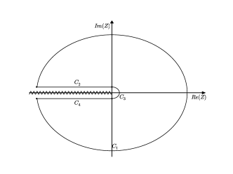
If and are the number of zeros and poles of , respectively, inside the contour (taken to be anticlockwise), then
| (137) |
Let’s evaluate the left hand side of (137) for each contour separately:
- 1.
-
2.
& : Since the values of above and under the cut are complex conjugate of each other, the contribution from these diagrams can be added together to get
(139) where is an infinitesimal positive number.
If we define , the right hand side of (2) (apart from the factor of ) measures how much rotates from to . Since on the whole negative real line, is definable on one Riemann sheet. Combining this result with and , we get
(140) -
3.
: IR conditions require that close to , . This means
(141)
Adding the values of all the contours and considering the fact that is finite everywhere (), we conclude that the number of zeros of in complex plane of (inside contour ) is zero. Since there is no zero on the negative real line (), there is no zero of in the complex plane of except the one at . Therefore, stability has been proven.
Appendix B FDT
Here, we present the proof of (52) 999Most of the content of this appendix is taken from Birrell and Davies (1984).. Let’s start by the following definitions
| (142) | |||||
| (143) | |||||
| (144) | |||||
| (145) | |||||
| (146) |
where is anti-commutator and shows expectation value in a quantum state. If we define
| (147) |
| (148) |
we get the following relations
| (149) | |||||
| (150) | |||||
| (151) | |||||
| (152) |
For a translational invariant system, the value of all the two point functions depend only on space-time separation. This will allow us to define the following Fourier transform with respect to time
| (153) |
Now, let us assume that the quantum system is in thermal state with temperature . It requires that
| (154) |
resulting in the following relation in Fourier space
| (155) |
Using (149), we get
| (156) | |||
| (157) |
On the other hand, since and are time transpose of each other, in Fourier space they are complex conjugate. As a result,
| (158) | |||||
where and are imaginary part and real part respectively and in the second line we have used the positivity of two point function (resulting that and are real.)
With the assumption that this field theory in Hilbert space representation has an equivalent representation in terms of double path integral, time ordered two point function is given by (46). In Fourier space, it reads
| (159) |
is a total imaginary number and is a real number. As a result,
| (160) |
Combining (149)(158)(160) we arrive at
| (161) |
which reduces to (52) at zero temperature.
Appendix C Quantum Transition
We start by proving a simple theorem for any quantum system. Consider a quantum mechanical system in the (normalized) initial state evolves in time and the probability of finding the system at a later time in the state is called , and assume ’s are orthonormal:
| (162) |
where is the time evolution operator.
Now, consider a (normalized) state as a superposition of states:
| (163) | |||
Probability of measuring the system at time in the state is given by
| (164) |
Then,
| (165) | |||||
where we have used the triangular inequality in the second line. So is bounded from above by .
Now, let’s get back to the scattering of a massless particle with state , a superposition of different masses, in Section VI.3. We already have shown (see (95)) that defined as transition probability of a massless particle scattering with a massive particle (mass ) scales with as
| (166) |
where depends on the momentum of the particles but independent of . Using (165) for transition probabilities, we conclude that
| (167) |
where is the maximum of ’s.