Magnetic axis safety factor of finite $\beta$ spheromaks and transition from spheromaks  to toroidal magnetic bubbles

Abstract

The value of the safety factor on the magnetic axis of a finite-beta spheromak is shown to be a function of beta in contrast to what was used in P. M. Bellan, Phys. Plasmas 9, 3050 (2002); this dependence on beta substantially reduces the gradient of the safety factor compared to the previous calculation. The method for generating finite-beta spheromak equilibria is extended to generate equilibria describing toroidal magnetic “bubbles” where the hydrodynamic pressure on the magnetic axis is less than on the toroid surface. This ”anti-confinement” configuration can be considered an  equilibrium with an inverted beta profile and is relevant to interplanetary magnetic clouds as these clouds have lower hydrodynamic pressure in their interior than on their surface.

I Introduction  

In Ref. Bellan (2002), one of the authors (PMB) examined analytic forms of finite $\beta$ spheromak equilibria and used a well-known expression for the value of the safety factor $q$ on the magnetic axis, denoted as $q_{axis}$,   to argue that finite $\beta$ causes the beneficial effect of a much larger $q\$gradient than when $\beta=0$. However, co-author (RP) numerically calculated $q_{axis}$ for these finite $\beta$ analytic equilibria and found numerical results substantially different from the $q_{axis}$ given in Ref.Bellan (2002). The reasons for this difference are identified as resulting from a subtle misuse of an expression for $q_{axis}.$ Resolution of this issue revealed that the analytic equilibria presented in Ref.Bellan (2002) could be extended to give an interesting toroidal equilibria where    the pressure on the magnetic axis of a toroid is lower than the pressure at the surface (edge) of the toroid rather than higher as in a tokamak; i.e., the beta profile is inverted and the configuration is bubble-like. Increase of a parameter $\bar{\gamma}$ (to be defined below) results in solutions to a Grad-Shafranov equation evolving from characterizing finite $\beta$ spheromak equilibria, to a conventional zero $\beta~{}$spheromak, to magnetic “bubbles” which are tokamak-like configurations having inverted $\beta$ profiles, and then to a tokamak with conventional $\beta$ profile. This evolution is characterized by the ratio of two Bessel functions changing sign as their argument $\bar{\gamma}$ is progressively increased. Interplanetary magnetic clouds are an example of the magnetic bubble situation because on the magnetic axis these clouds have lower hydrodynamic pressure than at their edge. Magnetic clouds have been previously modeled using numerical solutions to Grad-Shafranov equations Sonnerup et al. (2006),Hu et al. (2013) in a slab approximation (i.e., equations are solved in Cartesian geometry in the $xy$ plane with the $z$ direction ignorable); the model presented here differs by being analytic and axisymmetric (i.e., equations are solved in cylindrical geometry in the $rz$ plane with the $\phi$ direction ignorable) so that, in contrast to a slab approximation, toroidal geometry effects are inherently included. The analytic model has only a few parameters and so has less freedom than a numerical model but nevertheless has the useful feature of revealing parametric dependence and scaling. The analytic model also offers the possibility of providing a useful framework for other calculations, for example, calculating particle orbits in an axisymmetric cloud; the virtues of developing a repertoire of analytic solutions to the Grad-Shafranov equation has been discussed in Ref.Cerfon and Freidberg (2010).

II Basic relations

We use  a cylindrical coordinate system $\{r,\phi,z\}$ and consider the general axisymmetric magnetic field

$$\mathbf{B}=\frac{1}{2\pi}\nabla\psi\times\nabla\phi+B_{\phi}r\nabla\phi$$ (1)

where $\psi$ is the poloidal flux function and $B_{\phi}$ is the toroidal field. The $\phi$ direction is called the toroidal direction and any direction lying in the poloidal plane ($rz$ plane) is called a poloidal direction. From Ampere’s law the associated current density is

$$\mathbf{J}=\frac{1}{2\pi\mu_{0}}\nabla\left(B_{\phi}r\right)\times\nabla\phi-\frac{r^{2}\nabla\phi}{2\pi\mu_{0}}\nabla\cdot\left(\frac{1}{r^{2}}\nabla\psi\right).$$ (2)

We are interested in configurations where the poloidal flux function has a local extremum in the $r,z$ plane; both spheromaks and tokamaks are this type of configuration. The location of this extremum is called the magnetic axis and its vertical location defines the $z$ origin while its radial location is defined to be $r_{axis};$ $\psi$ is thus at a maximum or a minimum at $r=r_{axis},$ $z=0.$ If $\psi$ is at a maximum on the magnetic axis then $J_{\phi}$ is positive at the axis whereas if $\psi$ is at a minimum on the magnetic axis then $J_{\phi}$ is negative at the axis.

Spheromaks and tokamaks are characterized by the safety factor $q$ which is the number of times a field line goes around toroidally for each time it goes poloidally around the magnetic axis. Tokamaks typically have near-unity $q$ on the magnetic axis with $q$ increasing with increasing distance from the magnetic axis whereas spheromaks have near-unity $q$ on the magnetic axis and $q$ decreasing on moving away from the magnetic axis. The    gradient of $q,$ denoted as $q^{\prime},$ provides stability properties and detailed calculations show that a zero $\beta$ spheromak has small $q^{\prime}.$

The safety factor at the magnetic axis is given by Bellan (2000)

$$q_{axis}=\ \frac{\ e^{1/2}+e^{-1/2}}{r_{axis}}\frac{B_{\phi,axis}}{\mu_{0}J_{\phi,axis}\ }\$$ (3)

where

$$e=\left(\frac{\psi_{rr}}{\psi_{zz}}\right)_{axis}\$$ (4)

is a measure of the ellipticity of $\psi(r,z)~{}$in the vicinity of the magnetic axis such that $e>1$ corresponds to vertically elongated equilibria (prolate) while $e<1$ corresponds to vertically shortened equilibria (oblate). The force-free relation $\mu_{0}J_{\phi,axis}/B_{\phi,axis}=\lambda$ was invoked in Ref. Bellan (2000) to give $q_{axis}=\left(e^{1/2}+e^{-1/2}\right)/(\lambda r_{axis})$ but this result is valid only if the plasma is indeed force-free (i.e., has zero $\beta$ and equilibrium given by $\nabla\times\mathbf{B}=\lambda\mathbf{B}$). If $\beta$ is finite, then $\mu_{0}J_{\phi,axis}\neq\lambda B_{\phi,axis}$ and it is necessary to calculate the actual value of $\mu_{0}J_{\phi,axis}/B_{\phi,axis}$ by consideration of the details of the finite $\beta$ equilibrium.

To do this, we start by defining $\beta_{rel}$

$$\beta_{rel}=\mu_{0}\frac{P_{axis}-P_{lc}}{B_{axis}^{2}}$$ (5)

where $P_{axis}$ and $P_{lc}$ are respectively the hydrodynamic pressures on the magnetic axis and on the last closed flux surface. Positive $\beta_{rel}$ thus corresponds to a conventional $\beta$ profile whereas negative $\beta_{rel}$ corresponds to an inverted $\beta$ profile. This definition differs from that used in Ref. Bellan (2002) because (i) here $B_{axis}^{2}$ is used and (ii) a relative rather than absolute pressure is used. The definition in Ref. Bellan (2002) used, in contrast, the average poloidal field linking the circular surface lying in the $z=0$ plane between the geometric axis and the magnetic axis. Because the definition of $\beta_{rel}$ uses the relative hydrodynamic pressure, it is seen that $\beta_{rel}$ can be positive or negative. In particular, if $P_{axis}$ is smaller then $P_{lc},$ then $\beta_{rel}$ will be negative. The definition of $\beta_{rel}$ is useful because it provides a simple mathematical way to distinguish toroidal equilibria with inverted $\beta$ profiles   from those with normal $\beta$ profiles.   The former are toroidal magnetic bubbles while the latter are toroidal confinement configurations such as spheromaks and tokamaks.

On expressing the magnetic field as

$$\mathbf{B}=\frac{1}{2\pi}\left(\nabla\psi(r,z)\times\nabla\phi+\mu_{0}I(r,z)\nabla\phi\right)$$ (6)

where $I=2\pi rB_{\phi}/\mu_{0}$ is the poloidal current, MHD equilibrium $\mathbf{J\times B}=\nabla P$ can be expressed as the Grad-Shafranov equation Grad and Rubin (1958); Shafranov (1966)

$$r\frac{\partial}{\partial r}\left(\frac{1}{r}\frac{\partial\psi}{\partial r}\right)+\frac{\partial^{2}\psi}{\partial z^{2}}+4\pi^{2}\mu_{0}r^{2}\frac{dP}{d\psi}+\mu_{0}^{2}I\frac{dI}{d\psi}=0.$$ (7)

We assume that $P$ is a linear function of the poloidal flux $\psi$ and so can be expressed as

$$P=\frac{P_{axis}-P_{lc}}{\left(\psi_{axis}-\psi_{lc}\right)}\psi-\frac{P_{axis}\psi_{lc}-P_{lc}\psi_{axis}}{\left(\psi_{axis}-\psi_{lc}\right)}$$ (8)

where $\psi_{lc}$ is the last closed flux surface of the configuration.

The poloidal current is similarly assumed to be a linear function of the poloidal flux and can be expressed as

$$\mu_{0}I=\lambda\psi.$$ (9)

We note that the assumed linear dependence in Eq.9 differs from the assumption used in Solov’ev-type solutions such as in Ref.Cerfon and Freidberg (2010)  where it is assumed that $I^{2}\sim\psi+const.$ For the linear dependence assumed here, $IdI/d\psi$ is linear in $\psi$ whereas for the Solov’ev-type assumption, $IdI/d\psi$ is a constant.

Using Eq.9, the toroidal component of Eq.6 gives

$$B_{\phi,axis}=\frac{\lambda\psi_{axis}}{2\pi r_{axis}}.$$ (10)

The gradient of $P$ with respect to $\psi$ can then be expressed in terms of $\beta_{rel}$ as

$$\frac{dP}{d\psi}=\beta_{rel}\frac{B_{axis}^{2}}{\mu_{0}\psi_{axis}\left(1-\psi_{lc}/\psi_{axis}\right)}.$$ (11)

Since $B_{pol}$ vanishes at the magnetic axis, $B_{axis}^{2}=B_{\phi,axis}^{2}$ and so

$$\frac{dP}{d\psi}=\beta_{rel}\frac{\lambda^{2}\psi_{axis}}{4\pi^{2}r_{axis}^{2}\mu_{0}\left(1-\psi_{lc}/\psi_{axis}\right)}.$$ (12)

  

III Cylindrical Solutions to Finite $\beta_{rel}$ Grad-Shafranov Equation

We now introduce dimensionless quantities

$$\bar{\psi}=\frac{\psi}{\psi_{axis}},\text{ }\bar{r}=\frac{r}{r_{axis}},\text{ }\bar{z}=\frac{z}{r_{axis}},\text{ }\bar{\lambda}=\lambda r_{axis}$$ (13)

so Eq.7 can be expressed as

$$\ \bar{r}\frac{\partial}{\partial\bar{r}}\left(\frac{1}{\bar{r}}\frac{\partial\bar{\psi}}{\partial\bar{r}}\right)+\ \frac{\partial^{2}\bar{\psi}}{\partial\bar{z}^{2}}+\ \bar{\lambda}^{2}\left(\frac{\beta_{rel}\bar{r}^{2}}{\ 1-\bar{\psi}_{lc}}+\ \bar{\psi}\right)=0.$$ (14)

We define

$$\bar{\chi}=\frac{\beta_{rel}\bar{r}^{2}}{\left(1-\bar{\psi}_{lc}\right)}+\bar{\psi}$$ (15)

so Eq.14 becomes

$$\ \bar{r}\frac{\partial}{\partial\bar{r}}\left(\frac{1}{\bar{r}}\frac{\partial\bar{\chi}}{\partial\bar{r}}\right)+\ \frac{\partial^{2}\bar{\chi}}{\partial\bar{z}^{2}}+\ \bar{\lambda}^{2}\bar{\chi}=0.$$ (16)

We assume a solution of the form

$$\bar{\chi}=\bar{r}g(\bar{r})\cos(\bar{k}\bar{z})$$ (17)

so Eq.16 becomes

$$\ \frac{\partial^{2}g}{\partial\bar{r}^{2}}+\frac{1}{\bar{r}}\frac{\partial g}{\partial\bar{r}}+\left(\bar{\gamma}^{2}-\frac{1}{\bar{r}^{2}}\right)g=0$$ (18)

where

$$\bar{\gamma}^{2}=\bar{\lambda}^{2}-\bar{k}^{2}.$$ (19)

Equation 18 is Bessel’s equation with general solution for real $\bar{\gamma}$

$$g(\bar{r})=\sigma_{J}J_{1}(\bar{\gamma}\bar{r})+\sigma_{Y}Y_{1}(\bar{\gamma}\bar{r})$$ (20)

where $\sigma_{J}$ and $\sigma_{Y}$ are constant coefficients to be determined by boundary conditions.

From Eqs.15 and 17 the solution to the normalized Grad-Shafranov equation is

$$\bar{\psi}=\bar{r}\left(\sigma_{J}J_{1}(\bar{\gamma}\bar{r})+\sigma_{Y}Y_{1}(\bar{\gamma}\bar{r})\right)\cos(\bar{k}\bar{z})-\bar{r}^{2}Q\$$ (21)

where

$$Q=\frac{\beta_{rel}}{1-\bar{\psi}_{lc}}.$$ (22)

However, $\bar{\psi}=1$ is required at $\bar{r}=1,$ $\bar{z}=0$ (i.e., at the magnetic axis) so

$$\sigma_{J}J_{1}(\bar{\gamma})+\sigma_{Y}Y_{1}(\bar{\gamma})=1+Q\ .\$$ (23)

The following three Bessel identities where $C_{n}=J_{n}$ or $Y_{n}$ will now be used repeatedly in the rest of the discussion:

$$\frac{dC_{0}(s)}{ds} =-C_{1}(s)$$ (24a)

$$\frac{d}{ds}\left(sC_{1}(s)\right) =sC_{0}(s)$$ (24b)

$$sC_{2}(s)\ =2C_{1}(s)-sC_{0}(s)\ .$$ (24c)

The magnetic axis is also where $$\partial\bar{\psi}/\partial\bar{r} \bar{r}, \bar{r}=1 \bar{z}=0$$ vanishes and so taking the derivative of Eq.21 with respect to using Eq.24b, and then setting and gives

$$\ \sigma_{J}J_{0}(\bar{\gamma})+\sigma_{Y}Y_{0}(\bar{\gamma})=\frac{2}{\bar{\gamma}}Q.$$ (25)

Equations 23 and 25 constitute two linear inhomogeneous algebraic equations for the coefficients $\sigma_{J}$ and $\sigma_{Y}.$ Solving these equations for $\sigma_{J}$ and $\sigma_{Y}$ and using the Wronskian

$$J_{1}(s)Y_{0}(s)-J_{0}(s)\ Y_{1}(s)\ =\frac{2}{\pi s}$$ (26)

and Eq.24c gives

$$\sigma_{J} =\frac{\pi\bar{\gamma}}{2}\left(Y_{0}(\bar{\gamma})-QY_{2}\left(\bar{\gamma}\right)\right)$$ (27a)

$$\sigma_{Y} =\frac{\pi\bar{\gamma}}{2}\left(-J_{0}(\bar{\gamma})+QJ_{2}(\bar{\gamma})\right).$$ (27b)

IV Spheromak-type solutions

Spheromaks are singly-connected Grad-Shafranov equilibria (i.e., there is no “hole” in the “doughnut”) and so the domain includes $\bar{r}=0.$ A spheromak therefore cannot contain a $Y_{1}(\bar{\gamma}\bar{r})$ component because $Y_{1}(\bar{\gamma}\bar{r})$ diverges at $\bar{r}=0.$ It is thus necessary to impose $\sigma_{Y}=0$ for a spheromak in which case Eq.27b yields the relation

$$Q=\frac{J_{0}(\bar{\gamma})}{J_{2}(\bar{\gamma})}.$$ (28)

Substituting for $Q$ in Eq.27a and using Eqs.24c and 26 gives

$$\sigma_{J}=\frac{2}{\bar{\gamma}J_{2}(\bar{\gamma})}.$$ (29)

Using Eq.24c to substitute for $J_{2}(\bar{\gamma})$ in Eq.28 shows that Eq.28 can alternately be written as

$$Q=\frac{2J_{1}(\bar{\gamma})}{\bar{\gamma}J_{2}(\bar{\gamma})}-1$$ (30)

so one can also write $\sigma_{J}$ as

$$\sigma_{J}=\ \frac{1+Q}{J_{1}(\bar{\gamma})}.$$ (31)

Because $\sigma_{Y}=0$ for a spheromak Eqs.22 and 28 show   that a spheromak has

$$\beta_{rel}=\frac{J_{0}(\bar{\gamma})}{J_{2}(\bar{\gamma})}\left(1-\bar{\psi}_{lc}\right)\$$ (32)

and

$$\sigma_{J}=\frac{1}{J_{1}(\bar{\gamma})}\left(1+\frac{\beta_{rel}}{1-\bar{\psi}_{lc}}\right).$$ (33)

On substituting for $\sigma_{J}$ and $Q$ in Eq.21 the solution to the normalized Grad-Shafranov equation becomes

$$\bar{\psi}=\bar{r}\frac{J_{1}(\bar{\gamma}\bar{r})}{J_{1}(\bar{\gamma})}\left(1+\frac{\beta_{rel}}{1-\bar{\psi}_{lc}}\right)\cos(\bar{k}\bar{z})-\bar{r}^{2}\frac{\beta_{rel}}{1-\bar{\psi}_{lc}}$$ (34)

If $\beta_{rel}=0$ and $\bar{\psi}_{lc}=0\$are additionally assumed, the standard result for a zero-beta spheromak in a cylindrical flux conserver of radius $a$ is retrieved, namely $\bar{\gamma}=x_{01}=2.405$ where $x_{01}$ is the first root of $J_{0}.$ Since $\bar{\gamma}=\gamma r_{axis},~{}$and the last closed flux surface is at the cylinder radius, then the assumption $\bar{\psi}_{lc}=0$ and $\beta_{rel}=0$ in Eq. 34 implies $J_{1}(\gamma a)=0$ in which case  $\gamma a=x_{11}=3.83$ where $x_{11}$ is the first root of $J_{1}.$ Thus, for a $\beta_{rel}=0$ spheromak, $r_{axis}/a=\bar{\gamma}/(\gamma a)=x_{01}/x_{11}=\allowbreak 0.63\$as is well known. Equation 32 shows that spheromaks with finite positive $\beta_{rel}$ are restricted to the range $0<\bar{\gamma}<2.405$ but, as will be discussed in Sec.VI, physically relevant non-spheromak configurations with negative $\beta_{rel}$ exist when $\bar{\gamma}>2.405.$

Substitution of Eq.32 into Eq.34 gives

$$\bar{\psi}=\frac{1}{J_{2}(\bar{\gamma})}\left(\frac{2\bar{r}}{\bar{\gamma}}J_{1}(\bar{\gamma}\bar{r})\cos(\bar{k}\bar{z})-\bar{r}^{2}J_{0}(\bar{\gamma})\right)$$ (35)

which reverts to the $\beta_{rel}=0$ solution when $\bar{\gamma}=2.405$ as can be seen using Eq.24c to give $\bar{\gamma}J_{2}(\bar{\gamma})=2J_{1}(\bar{\gamma})$ if $J_{0}(\bar{\gamma})=0$.

V Safety Factor of Spheromaks with finite $\beta_{rel}$

The last closed flux surface of a spheromak has $\bar{\psi}_{lc}=0$ and $P_{lc}=0$ in which case Eqs. 5 and 10 give

$$\beta_{rel}=4\pi^{2}r_{axis}^{2}\frac{\mu_{0}P_{axis}}{\lambda^{2}\psi_{axis}^{2}}$$ (36)

and Eq.34 becomes

$$\bar{\psi}=\bar{r}\frac{J_{1}(\bar{\gamma}\bar{r})}{J_{1}(\bar{\gamma})}\left(1+\beta_{rel}\right)\cos(\bar{k}\bar{z})-\beta_{rel}\bar{r}^{2}$$ (37)

which is the same as Eq.(2) of Ref. Bellan (2002) except for the different definition of $\beta_{rel}.$

In order to determine $q_{axis},$ Eq.3  shows that it is necessary to calculate $\mu_{0}J_{\phi,axis}/B_{\phi,axis}.$ Equation 2 shows that

$$\mu_{0}J_{\phi}=-\frac{\psi_{axis}}{2\pi\bar{r}r_{axis}^{3}}\left[\bar{r}\frac{\partial}{\partial\bar{r}}\left(\frac{1}{\bar{r}}\frac{\partial\bar{\psi}}{\partial\bar{r}}\right)+\ \frac{\partial^{2}\bar{\psi}}{\partial\bar{z}^{2}}\right]$$ (38)

so, using Eq.10 and Eq.14 it is seen that

$$\frac{\mu_{0}J_{\phi,axis}}{B_{\phi,axis}}=\left(1+\beta_{rel}\right)\lambda.$$ (39)

Thus $\mu_{0}J_{\phi,axis}/B_{\phi,axis}=\lambda$ only if $\beta_{rel}=0.$ Inserting Eq.39 in Eq.3 gives

$$q_{axis}=\ \frac{\ e^{1/2}+e^{-1/2}}{\bar{\lambda}\left(1+\beta_{rel}\right)}\$$ (40)

which differs from Eq.(30) of Ref.Bellan (2002) by having an extra and important factor of $(1+\beta_{rel})$ in the denominator.

From Eq.35 and use of the Bessel identities it is seen that

$$\left(\bar{\psi}_{zz}\right)_{axis} =-\frac{2\bar{k}^{2}}{\bar{\gamma}\ }\frac{J_{1}(\bar{\gamma})}{J_{2}(\bar{\gamma})}$$ (41a)

$$\left(\bar{\psi}_{rr}\right)_{axis} =\frac{-2\bar{\gamma}J_{1}(\bar{\gamma})}{J_{2}(\bar{\gamma})}$$ (41b)

so the ellipticity is

$$e=\frac{\bar{\gamma}^{2}}{\bar{k}^{2}}.$$ (42)

This indicates that the poloidal flux surfaces will be circular near the magnetic axis (i.e., have $e=1$) if $\bar{\gamma}=\bar{k}$ in which case $\bar{\lambda}=\sqrt{2}\bar{\gamma}.$ Combination of Eqs.32, 40, and 42 gives

$$q_{axis}=\ \frac{\bar{\lambda}}{\bar{\gamma}\bar{k}}\frac{1}{1+\beta_{rel}}=\ \frac{\bar{\lambda}}{2\bar{k}}\frac{J_{2}(\bar{\gamma})}{J_{1}(\bar{\gamma})}.$$ (43)

Equation 43 has been validated by direct numerical integration of field lines in the vicinity of the magnetic axis of a magnetic configuration characterized by Eq.6 with $\bar{\psi}$ given by Eq.35.   In the $\beta_{rel}=0\$limit, $J_{0}(\bar{\gamma})=0$ and $q_{axis}\rightarrow\bar{\lambda}/\left(\bar{\gamma}\bar{k}\right)$ which is Eq.(33) of Ref.Bellan (2002), but for finite positive $\beta_{rel},$ Eq. 43 shows that $q_{axis}$ is reduced from its $\beta_{rel}=0$ value.

The safety factor at the wall is Bellan (2002)

$$q_{wall}=\frac{\bar{\lambda}}{2\pi\bar{k}}\cos^{-1}\left(J_{0}(\bar{\gamma})\right)$$ (44)

and so the ratio of safety factor at the wall to that at the axis is

$$\frac{q_{wall}}{q_{axis}}=\frac{J_{1}(\bar{\gamma})}{J_{2}(\bar{\gamma})}\frac{\cos^{-1}\left(J_{0}(\bar{\gamma})\right)}{\pi}$$ (45)

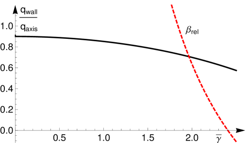
Figure 1: $q_{wall}/q_{axis}$ plotted as black solid line v. $\bar{\gamma}$ from Eq.45 and $\beta_{rel}$ plotted as red dashed line.

which is plotted in Fig.1. Contrary to Ref.Bellan (2002) it is seen that the shear (difference between $q_{wall}$ and $q_{axis})$ decreases with increasing $\beta_{rel}$ (i.e., with $\bar{\gamma}$ decreasing below 2.405). Using $i\theta=\ln\left(\cos\theta+i\sin\theta\right)$ to write

$$\cos^{-1}\left(J_{0}(\bar{\gamma})\right)=-i\ln\left(J_{0}(\bar{\gamma})+i\sqrt{1-\left(J_{0}(\bar{\gamma})\right)^{2}}\right)$$ (46)

and then using $J_{0}(\bar{\gamma})=1-\bar{\gamma}^{2}/4$ for $\bar{\gamma}\ll 1$, it is seen that for $\bar{\gamma}\ll 1$

$$\cos^{-1}\left(J_{0}(\bar{\gamma})\right)\simeq-i\ln\left(1-\frac{\bar{\gamma}^{2}}{4}+i\frac{\bar{\gamma}}{\sqrt{2}}\right)\simeq\frac{\bar{\gamma}}{\sqrt{2}}.$$ (47)

Since $J_{1}(\bar{\gamma})\simeq\bar{\gamma}/2$ and $J_{2}(\bar{\gamma})\simeq\bar{\gamma}^{2}/8$ for $\bar{\gamma}\ll 1,$ Eq.45 has the limiting behavior

$$\ \frac{q_{wall}}{q_{axis}}\rightarrow\frac{4}{\sqrt{2}\pi}=0.900\text{ for }\bar{\gamma}\ll 1$$ (48)

which is seen in Fig. 1. Furthermore, Eq.32 has the limiting behavior

$$\ \beta_{rel}\rightarrow\frac{8}{\bar{\gamma}^{2}}\text{ for }\bar{\gamma}\ll 1;$$ (49)

i.e., $\beta_{rel}$ diverges at small $\bar{\gamma}\$ which is also seen in Fig. 1.

We note that numerical calculations reported in Ref.Gautier et al. (1981) assumed $I^{2}\sim\psi^{2}(1+2\alpha\psi/3)$ and $dP/d\psi\sim\psi-\psi_{0}$ in a spherical geometry and found that the gradient of the shear had a strong dependence on $\alpha.$ The analytic solution given here would correspond approximately to the $\alpha=0$ numerical solution reported in Ref.Gautier et al. (1981); the correspondence is not exact because of the different assumptions for the dependence of $P$ on $\psi$, the shape of the boundary (cylinder v. sphere), and the assumption of a central hole in Ref. Gautier et al. (1981).

VI Toroidal magnetic bubble: Negative $\beta_{rel}$

We now consider the situation where $\beta_{rel}<0$ and $\bar{\psi}_{lc}\neq 0.$ We consider the $\sigma_{Y}=0$ case first as was assumed for spheromaks and then later consider the more general case where both $\sigma_{J}$ and $\sigma_{Y}$ are finite.

VI.1 $\sigma_{Y}=0$ case

In the $\sigma_{Y}=0$ case $\bar{\psi}(\bar{r},\bar{z})$ is mathematically identical to the spheromak solution considered in Sec.IV, i.e., Eq.35 provides the relevant flux function. The difference here is that $\bar{\psi}_{lc}$ is no longer assumed to be zero. Plots of $\bar{\psi}(\bar{r},\bar{z})$ using $\bar{\gamma}>2.405$ show that $\bar{\psi}(\bar{r},0)$ has periodic maxima and minima because of its $J_{1}(\bar{\gamma}\bar{r})$ dependence. Equation 13 defined $\bar{\psi}$ to be unity on the magnetic axis, i.e., $\bar{\psi}(\bar{r},0)=1$ at $\bar{r}=1$ and the magnetic axis was defined to be where $\bar{\psi}$ was a maximum or minimum. Because of the oscillatory behavior of Bessel functions, maxima or minima of $\bar{\psi}\,\$occur not only at $r=1$ but also for $\bar{r}>1.$ However, the maxima and minima occurring where $\bar{r}>1$ do not have $\bar{\psi}=1$ and so do not satisfy the $\bar{\psi}\ =1$ condition given in Eq.13. Thus, only the maximum of $\bar{\psi}(\bar{r},0)$ at $\bar{r}=1$ will be considered since maxima or minima at larger $\bar{r}$ do not satisfy the $\bar{\psi}\ =1$ requirement stipulated in Eq.13.

Examination of Eq.35 shows that $\bar{\psi}$ is independent of $\bar{z}$ if $J_{1}(\bar{\gamma}\bar{r})=0;$ at this radius $\bar{r}=x_{11}/\bar{\gamma}$ where $x_{11}=3.832$ is the first root of $J_{1}.$ We now show that this radius $\bar{r}=x_{11}/\bar{\gamma}$ is infinitesimally larger than the radius of the last closed flux surface. Since $\bar{\psi}$ is independent of $\bar{z}$    when $J_{1}(\bar{\gamma}\bar{r})=0,$ the flux surface passing through $\bar{r}=x_{11}/\bar{\gamma},$ $\bar{z}=0$ must be a straight vertical line, i.e., $\bar{\psi}(x_{11}/\bar{\gamma},\bar{z})=\bar{\psi}(x_{11}/\bar{\gamma},0)$ for all $\bar{z}.$ Because a straight vertical line goes to $\bar{z}=\pm\infty$, the flux surface passing through $\bar{r}=x_{11}/\bar{\gamma},\bar{z}=0$ is open. Immediately to the left of this line the flux surfaces are closed and so the last closed flux surface is at the radius $\bar{r}_{lc}$ where

$$\bar{r}_{lc}=\lim_{\delta\rightarrow 0}\left(\frac{x_{11}}{\bar{\gamma}}-\delta\right)=\frac{x_{11}}{\bar{\gamma}}.$$ (50)

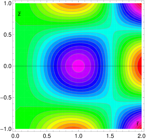
Figure 2: Contour plot of $\bar{\psi}(\bar{r},\bar{z})$ given by Eq.35 for $\bar{\gamma}=\bar{k}=2.5.$ The radius of the last closed flux surface is at $\bar{r}=1.53.$ The hydrodynamic pressure is lower in the pink region than in the green region so the configuration is a magnetic bubble.

This can also be seen graphically from the flux surface contours shown in Fig.2 (to be discussed in more detail later) where it is seen that a straight vertical line separatrix lies between the blue-purple closed flux surfaces having magnetic axis at $\bar{r}=1,$ $\bar{z}=0$ and the green-orange flux surfaces to the right. Equation 50 gives the radial location of this vertical line.

A toroidal inverse aspect ratio (ratio of torus minor to major radius) can be defined as

$$\varepsilon=\frac{r_{lc}-r_{axis}}{r_{axis}}=\bar{r}_{lc}-1=\frac{x_{11}-\bar{\gamma}}{\bar{\gamma}}.$$ (51)

Using $J_{1}(\bar{\gamma}\bar{r}_{lc})=0$ at the last closed flux surface, Eq. 35 may be evaluated at $\bar{r}=\bar{r}_{lc},\bar{z}=0$ to give

$$\bar{\psi}_{lc}=-\frac{x_{11}^{2}}{\bar{\gamma}^{2}}\frac{J_{0}(\bar{\gamma})}{J_{2}(\bar{\gamma})}.$$ (52)

Inserting $\bar{\psi}_{lc}$ in Eq.32 gives

$$\beta_{rel}=\left(1+\frac{x_{11}^{2}}{\bar{\gamma}^{2}}\frac{J_{0}(\bar{\gamma})}{J_{2}(\bar{\gamma})}\right)\frac{J_{0}(\bar{\gamma})}{J_{2}(\bar{\gamma})}.$$ (53)

In order to have $r_{lc}>r_{axis}$ Eq.51 shows that it is necessary to have $\bar{\gamma}<x_{11}=3.832.$ A plot of Eq.53 shows that $\beta_{rel}$ is negative if $2.405<\bar{\gamma}<3.736$; $\beta_{rel}$ changes sign at $\bar{\gamma}=3.736$ because the quantity in parenthesis in Eq.53 changes sign at $\bar{\gamma}=3.736.$ Thus if $2.405<\bar{\gamma}<3.736$, $\beta_{rel}$ is negative and also  $r_{lc}>r_{axis}.\$

Because the minimum of $(1+s)s$ occurs when $s=-1/2,$ identifying  $s=x_{11}^{2}J_{0}(\bar{\gamma})/\left(\bar{\gamma}^{2}J_{2}(\bar{\gamma})\right)$ it is seen that $\beta_{rel}$ is at a minimum when $x_{11}^{2}J_{0}(\bar{\gamma})/\left(\bar{\gamma}^{2}J_{2}(\bar{\gamma})\right)=-1/2$ in which case

$$\min\left[\beta_{rel}\right]=-\frac{\bar{\gamma}^{2}}{4x_{11}^{2}}.$$ (54)

  

Using the Bessel identities, the magnetic field components are  

$$B_{r} =-\frac{\psi_{axis}}{2\pi r_{axis}^{2}\bar{r}}\frac{\partial\bar{\psi}}{\partial\bar{z}}=\frac{\psi_{axis}}{2\pi r_{axis}^{2}\ }\frac{2\bar{k}\ }{\bar{\gamma}}\frac{J_{1}(\bar{\gamma}\bar{r})}{J_{2}(\bar{\gamma})}\sin(\bar{k}\bar{z})$$ (55a)

$$B_{\phi} =\frac{\lambda\psi}{2\pi r}=\ \frac{\psi_{axis}}{2\pi r_{axis}^{2}\ }\ \frac{\bar{\lambda}}{J_{2}(\bar{\gamma})}\left(\frac{2}{\bar{\gamma}}J_{1}(\bar{\gamma}\bar{r})\cos(\bar{k}\bar{z})-\bar{r}J_{0}(\bar{\gamma})\right)$$ (55b)

$$B_{z} =\frac{\psi_{axis}}{2\pi r_{axis}^{2}\bar{r}}\frac{\partial\bar{\psi}}{\partial\bar{r}}=\frac{\psi_{axis}}{2\pi r_{axis}^{2}}\ \frac{2}{J_{2}(\bar{\gamma})}\left(\ J_{0}(\bar{\gamma}\bar{r})\cos(\bar{k}\bar{z})-J_{0}(\bar{\gamma})\right).$$ (55c)

Using Eq.24c and Eq.55b it is seen that

$$B_{\phi,axis}=\frac{\psi_{axis}}{2\pi r_{axis}^{2}\ }\ \bar{\lambda}.$$ (56)

A normalized magnetic field can be defined as $\mathbf{\bar{B}=B(}\bar{r},\bar{z}\mathbf{)/}B_{\phi,axis}$ with components

$$\bar{B}_{r}(\bar{r},\bar{z}) =\frac{2\bar{k}\ }{\bar{\gamma}\bar{\lambda}}\frac{J_{1}(\bar{\gamma}\bar{r})}{J_{2}(\bar{\gamma})}\sin(\bar{k}\bar{z})$$ (57a)

$$\bar{B}_{\phi}(\bar{r},\bar{z}) =\frac{\frac{2}{\bar{\gamma}}J_{1}(\bar{\gamma}\bar{r})\cos(\bar{k}\bar{z})-\bar{r}J_{0}(\bar{\gamma})}{J_{2}(\bar{\gamma})\ }$$ (57b)

$$\bar{B}_{z}(\bar{r},\bar{z}) =\frac{2}{\bar{\lambda}\ }\frac{\left(J_{0}(\bar{\gamma}\bar{r})\cos(\bar{k}\bar{z})-J_{0}(\bar{\gamma})\right)}{J_{2}(\bar{\gamma})}.$$ (57c)

As required, both $$\bar{B}_{r} \bar{B}_{z} \bar{r}=1,\bar{z}=0 \bar{B}_{\phi}=1$$ and vanish on the magnetic axis (i.e., at ) and on the magnetic axis.

Equation 35 with $2.405<\bar{\gamma}<3.736$ thus gives the flux surface for a magnetic bubble, i.e., a toroidal configuration with closed field lines where the pressure on the magnetic axis is lower than the pressure at the surface of the toroid. The direction of the $\mathbf{J\times B}$ force is thus outwards rather than inwards in contrast to a tokamak. This configuration is relevant to axisymmetric interplanetary magnetic clouds ejected from the sun by coronal mass ejections. Spacecraft measurements indicate that $P$ is smaller in the interior of these clouds than outside   so these clouds have negative $\beta_{rel}.$ Another possible situation would be in the solar interior where a toroidal bubble configuration as described here would be a toroidal region of stronger magnetic field but reduced hydrodynamic pressure compared to the surroundings.

As a concrete example of such a configuration, consider the situation where $\bar{\gamma}=\bar{k}=2.5$ and $\bar{\lambda}=\sqrt{2}\bar{\gamma}.$ In this case $e=1$ so the poloidal flux surfaces are circular near the magnetic axis, the last closed flux surface is at $\bar{\psi}_{lc}=0.25$ and from Eq.53 $\beta_{rel}=-0.081.$ From Eq.51, it is seen that the inverse aspect ratio is $\varepsilon=\allowbreak 0.53.$ Figure 2 plots contours of $\psi(\bar{r},\bar{z})$ and it is seen that the last closed flux surface intersects $\bar{z}=0$ to the right of the magnetic axis at indeed $\bar{r}_{lc}=x_{11}/\bar{\gamma}=\allowbreak 1.\,\allowbreak 53.$ Figures 3, 4, 5, and 6 plot $\bar{\psi}(\bar{r},0),$ $\bar{B}_{\phi}(\bar{r},0),$ $\bar{B}_{z}(\bar{r},0),$ and $\bar{B}^{2}(\bar{r},0)\$respectively.

From Eq.5 it is seen that

$$\frac{\mu_{0}}{B_{axis}^{2}}P_{axis}=\frac{\mu_{0}}{B_{axis}^{2}}P_{lc}+\beta_{rel}$$ (58)

so the hydrodynamic pressure on the magnetic axis is lower than on the last closed flux surface. If $P_{axis}$ is set to zero, then the external pressure would be

$$\frac{\mu_{0}}{B_{axis}^{2}}P_{lc}=-\beta_{rel}$$ (59)

in which case the configuration would be a vacuum at the magnetic axis (zero plasma pressure) with increasing pressure going away from the magnetic axis toward last closed flux surface.

If $\bar{\gamma}$ is further increased, the sign of $\beta_{rel}$ can become positive again in which case the equilibrium will become tokamak-like (higher pressure on magnetic axis). Additional increase of $\bar{\gamma}$ will cause $\beta_{rel}$ to oscillate in sign giving a sequence of bubble-like and tokamak-like configurations. Also, for a given configuration one could elect to truncate the flux at some value larger than $\psi_{lc}$ and so obtain a smaller aspect ratio equilibrium. In accordance with the Shafranov virial theorem, any one of these configurations will involve a jump in the magnetic field at the surface of the toroid if it is assumed that at the surface the external magnetic field differs from the internal field. This jump corresponds to the existence of surface currents. In a tokamak these surface currents are provided by a set of coils immediately external to the toroidal volume and these coils are called the vertical field coils. The field produced by these coils is mainly in the $z$ direction and will be referred to here as $B_{z}^{ext}$. This field $B_{z}^{ext}$ constitutes a portion of the total field inside the toroidal volume and provides equilibrium in the major radius direction. This takes place via a radial force $\sim J_{\phi}B_{z}^{ext}$ directed towards $\bar{r}=0\$that balances the radially outward hoop force as well as some hydrodynamic pressure forces. The hoop force is a property of any toroidal current system and occurs because a toroidal current produces a stronger poloidal field near $\bar{r}=0$, $\bar{z}=0$ (inside) than at $\bar{r}=\bar{r}_{lc},$ $\bar{z}=0\$(outside). This stronger poloidal field on the inside compared to the outside corresponds to greater magnetic pressure on the inside than on the outside; for low $\beta$ the force resulting from magnetic pressure imbalance dominates any hydrodynamic pressure imbalance. Without the offsetting force provided by $B_{z}^{ext}$ the hoop force would act to expand the torus major radius.

At first sight it might appear that the flux contours in Fig.2 are such that the magnetic pressure is higher on the outside than on the inside because the midplane poloidal flux surfaces in Fig. 2 are more tightly packed outside the magnetic axis (e.g., at $\bar{r}\simeq 1.5)$ than inside the magnetic axis (e.g., at $\bar{r}\simeq 0.25$). However, the density of field lines and hence the poloidal field is nevertheless stronger inside the magnetic axis than outside because of the inverse $\bar{r}$ dependence in $B_{z}=(2\pi r)^{-1}\partial\psi/\partial r$. The twice as tight midplane flux surface packing in Fig. 2 at $\bar{r}\simeq 1.5\$ compared to at $\bar{r}\simeq 0.25$ gives a twice as large $\partial\psi/\partial r$ on the outside compared to the inside. However, this twice as tight radial packing is overcome by the $(2\pi r)^{-1}$ factor, a toroidal geometry effect that produces an approximately six-fold inside-to-outside enhancement with the net result that $\left|B_{z}\right|$ is about three times larger at $\bar{r}\simeq 0.25$ than at $\bar{r}\simeq 1.5$. This three-fold inside-to-outside ratio of $\left|B_{z}\right|$ is evident in Fig. 5.   

In order to have the $B_{z}^{ext}$ required  for equilibrium, it would be necessary to have surface currents flowing on the surface of the toroid. Since there are no powered coils to sustain surface currents exterior to a magnetic cloud, it is unlikely that such surface currents would exist in the magnetic cloud context. Without the $B_{z}^{ext}$ provided by surface currents  (and intrinsic to the equilibrium given here), the hoop force resulting from the imbalance between $B_{z}^{2}$ on the inside and $B_{z}^{2}$ on the outside will cause the major radius of magnetic clouds to increase with time. The difference between poloidal flux surfaces with and without incorporation of $B_{z}^{ext}$ is of the order of the inverse aspect ratio $\varepsilon$ because $B_{z}^{ext}\$ is a toroidal effect and so scales as $\varepsilon.$

VI.2 Finite $\sigma_{J}$ and $\sigma_{Y}$ case

The spheromak solution required $\sigma_{Y}$ to be zero to avoid singularity at $\bar{r}=0.$ The magnetic bubble solution discussed above used the same functional form as the spheromak solution (i.e., had $\sigma_{Y}=0$ and used Eq.34) and found that a tokamak-like solution with $\beta_{rel}<0$   (i.e., inverted beta profile) occurred if $2.405<\bar{\gamma}<3.736.$ If $\bar{r}=0$ is excluded from the domain so the configuration is doubly-connected, the singular nature of $Y_{1}(\bar{\gamma}\bar{r})$ at $\bar{r}=0$ is no longer a constraint and the more general solution given by Eqs. 21, 27a, and 27b can be used. The consequence of imposing $\sigma_{Y}=0$ was for Eq.27b to force the relationship  between $Q$ and $\bar{\gamma}$ given by Eq.28. If $\sigma_{Y}$ is not forced to be zero, then this relationship between $Q$ and $\bar{\gamma}$ is no longer imposed and the only remaining condition is that the domain must exclude $\bar{r}=0.$

Consideration of Eq.21 and recalling the discussion that led to Eq.50 shows that $\bar{\psi}(\bar{r}_{lc},\bar{z})$ is independent of $\bar{z}$ at $\bar{r}_{lc}$ where $\bar{r}_{lc}$ is now defined by

$$\sigma_{J}J_{1}(\bar{\gamma}\bar{r}_{lc})+\sigma_{Y}Y_{1}(\bar{\gamma}\bar{r}_{lc})=0.$$ (60)

Thus Eq.60 provides a radial shift of the location of the last closed flux surface and generalizes the discussion that led to Eq.50. Because $\sigma_{J}$ and $\sigma_{Y}$ depend on $\bar{\gamma}$ and on $Q$ (hence on $\beta_{rel}$), Eq.60 shows that $\bar{r}_{lc}$ depends on both $\bar{\gamma}$ and $\beta_{rel}.$ However, by assumption $\bar{r}_{lc}>1$ (last closed flux surface radius is to the right of the magnetic axis) which restricts the allowed values of $\bar{\gamma}$ and $\beta_{rel}$. Introduction of the $Y_{1}(\bar{\gamma}\bar{r})$ solution and the coefficients $\sigma_{J}$ and $\sigma_{Y}$ is thus analogous to generalizing the solution of some harmonic equation from being $\sin(kx)$ to being $\sin(kx+\Delta)=\sin(kx)\cos(k\Delta)+\cos(kx)\sin(k\Delta)$ where $\sin(kx)$, $\cos(kx)$ are the analogs of $J_{1}(\bar{\gamma}\bar{r}),Y_{1}(\bar{\gamma}\bar{r})$ and $\sigma_{J},\sigma_{Y}$ are the analogs of $\cos(k\Delta),\sin(k\Delta).$ Introducing finite $\Delta$ changes the phase of the solution and shifts the location of the solution.

Substitution for $\sigma_{J}$ and $\sigma_{Y}$ in Eq.60 using Eqs.27a, 27b gives

$$Q(\bar{\gamma},\bar{r}_{lc})=\frac{Y_{0}(\bar{\gamma})J_{1}(\bar{\gamma}\bar{r}_{lc})-J_{0}(\bar{\gamma})Y_{1}(\bar{\gamma}\bar{r}_{lc})}{Y_{2}\left(\bar{\gamma}\right)J_{1}(\bar{\gamma}\bar{r}_{lc})\ -J_{2}(\bar{\gamma})Y_{1}(\bar{\gamma}\bar{r}_{lc})}.$$ (61)

It is seen that Eq.61 reduces to Eq.28 if $J_{1}(\bar{\gamma}\bar{r}_{lc})=0$, i.e., the situation considered in Sec.VI.1 and that $Q$ becomes infinite when $\bar{r}_{lc}$ is  such that the denominator in the right hand side of Eq.61 vanishes.

Using Eqs.60 in Eq.21 it is seen that the last closed flux surface is given by

$$\bar{\psi}_{lc}=-\bar{r}_{lc}^{2}Q$$ (62)

and inserting this in Eq.22 gives

$$\beta_{rel}=Q+\bar{r}_{lc}^{2}Q^{2}.$$ (63)

The derivative of Eq.63 shows that the minimum possible $\beta_{rel}$ is $\beta_{rel}=-1/(4\bar{r}_{lc}^{2})$ which occurs when $Q=-1/(2\bar{r}_{lc}^{2});$ this generalizes  Eq.54.

Figure 7 plots the dependence of $Q$ and $\beta_{rel}$ on $\bar{r}_{lc}$ for $1<\bar{r}_{lc}<2$ with $\bar{\gamma}=2.5;$ it is seen that, as predicted, $\beta_{rel}$ has a minimum at $\beta_{rel}=-1/(4\bar{r}_{lc}^{2})$ which occurs when $Q=-1/(2\bar{r}_{lc}^{2}).$ It is also seen from this figure that when $\bar{r}_{lc}=x_{11}/\bar{\gamma}=1.5328$ the Sec.VI.1 result $\beta_{rel}=-0.081$ and $Q=J_{0}(\bar{\gamma})/J_{2}(\bar{\gamma})=$ $-0.108\$ is recovered. For this $\bar{\gamma}=2.5$ value the denominator in Eq.61 vanishes when $\bar{r}_{lc}\rightarrow 1.885.$

The following chain of dependence thus exists for doubly-connected configurations:

1. Independent values for $\bar{r}_{lc}$ and $\bar{\gamma}$ can be selected which then determine $Q$ via Eq. 61,

2. Using Eqs.27a and 27b in Eq.21 the flux function  $\bar{\psi}(\bar{r},\bar{z})$ is given by

   $$\bar{\psi}(\bar{r},\bar{z})=\frac{\pi}{2}\bar{\gamma}\bar{r}\left\{\begin{array}[c]{c}\,\left[Y_{0}(\bar{\gamma})-QY_{2}\left(\bar{\gamma}\right)\right]J_{1}(\bar{\gamma}\bar{r})\\ +\left[-J_{0}(\bar{\gamma})+QJ_{2}(\bar{\gamma})\right]Y_{1}(\bar{\gamma}\bar{r})\end{array}\right\}\cos(\bar{k}\bar{z})-\bar{r}^{2}Q,$$ (64)

3. $\beta_{rel}$ is given by Eq.63,

4. $\bar{\psi}_{lc}$ is given by Eq.62.

This chain of dependence for doubly-connected configurations differs from that of a finite $\beta$ spheromak. Specifically the chain of dependence for a finite $\beta$ spheromak is: $\bar{\psi}_{lc}=0$ is imposed because of the singly-connected topology, $\bar{r}_{lc}$ is determined from setting the left hand side of Eq.35  to zero on the midplane, and Eq.32 gives $\beta_{rel}=J_{0}(\bar{\gamma})/J_{2}(\bar{\gamma})$.

Another and equivalent point of view differentiating singly- and doubly-connected configurations from each other is the following:

(i) because the midplane of a singly-connected configuration contains $\bar{r}=0$ and because $\bar{\psi}=0$ at $\bar{r}=0$, the last closed flux surface for a singly-connected configuration must always have $\bar{\psi}=0,$

whereas in contrast,

(ii) because the midplane of a doubly-connected configuration excludes $\bar{r}=0,$ the last closed flux surface of a doubly-connected configuration cannot be $\bar{\psi}=0$ as such a flux surface would have to pass through $\bar{r}=0.$

The magnetic field components associated with Eq.64 normalized to $B_{\phi,axis}=\bar{\lambda}\psi_{axis}/\left(2\pi r_{axis}^{2}\right)$ are   

$$\bar{B}_{r}(\bar{r},\bar{z}) =\frac{\bar{k}}{\bar{\lambda}}\frac{\pi\bar{\gamma}}{2}\left\{\begin{array}[c]{c}\,\left[Y_{0}(\bar{\gamma})-QY_{2}\left(\bar{\gamma}\right)\right]J_{1}(\bar{\gamma}\bar{r})\\ +\,\left[-J_{0}(\bar{\gamma})+QJ_{2}(\bar{\gamma})\right]Y_{1}(\bar{\gamma}\bar{r})\end{array}\right\}\sin(\bar{k}\bar{z})$$ (65c)

$$\bar{B}_{\phi}(\bar{r},\bar{z}) =\frac{\pi\bar{\gamma}}{2}\left\{\begin{array}[c]{c}\,\left[Y_{0}(\bar{\gamma})-QY_{2}\left(\bar{\gamma}\right)\right]J_{1}(\bar{\gamma}\bar{r})\\ +\,\left[-J_{0}(\bar{\gamma})+QJ_{2}(\bar{\gamma})\right]Y_{1}(\bar{\gamma}\bar{r})\end{array}\right\}\cos(\bar{k}\bar{z})-\bar{r}Q$$ (65f)

$$\bar{B}_{z}(\bar{r},\bar{z}) =\frac{1}{\bar{\lambda}\ }\left(\frac{\pi\bar{\gamma}^{2}}{2}\left\{\begin{array}[c]{c}\,\left[Y_{0}(\bar{\gamma})-QY_{2}\left(\bar{\gamma}\right)\right]J_{0}(\bar{\gamma}\bar{r})\\ +\,\left[-J_{0}(\bar{\gamma})+QJ_{2}(\bar{\gamma})\right]Y_{0}(\bar{\gamma}\bar{r})\end{array}\right\}\cos(\bar{k}\bar{z})-2Q\right).$$ (65i)

Using Eqs.24c and 26 it is seen that Eq.65 reverts to Eq.57 when $$Q=J_{0}(\bar{\gamma})/J_{2}(\bar{\gamma}).$$

Acknowledgements: This material is based upon work supported by the U.S. Department of Energy Office of Science, Office of Fusion Energy Sciences under Award Numbers DE-FG02-04ER54755 and DE-SC0010471, by the National Science Foundation under Award Number 1059519, and by the Air Force Office of Scientific Research under Award Number FA9550-11-1-0184. The authors wish to thank an anonymous reviewer for making the valuable suggestion that $Y_{n}$ Bessel solutions be allowed when $\bar{r}=0$ is excluded from the domain.

Figure 3: Plot of $\bar{\psi}(\bar{r},0)$ as given by Eq.35 for $\bar{\gamma}=\bar{k}=2.5$ and $\bar{\lambda}=2\sqrt{\bar{\gamma}}.$ The radius of the last closed flux surface is at $\bar{r}=1.53\$and $\bar{\psi}_{lc}=0.25.$

Figure 4: $\bar{B}_{\phi}(\bar{r},0)$; Note that magnetic axis is at $\bar{r}=1.0$ and that maximum of $\bar{B}_{\phi}$ occurs to left of magnetic axis.

Figure 5: $\bar{B}_{z}(\bar{r},0);$ note that $\bar{B}_{z}$ changes sign at magnetic axis.

Figure 6: $\bar{B}_{r}^{2}+\bar{B}_{\phi}^{2}+\bar{B}_{z}^{2}$ as function of $\bar{r}$ for $\bar{z}=0.$

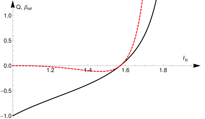
Figure 7: Figure 7. Blacksolid line is plot of $Q(\gamma,\bar{r}_{lc})$ as function of $\bar{r}_{lc}$ with $\bar{\gamma}=2.5;$ red dashed line is plot of $\beta_{rel}.$ For this $\bar{\gamma},$ $Q$ diverges when $\bar{r}_{lc}=1.885.$

References

- (1)
- (2)
- (3)
- (4)
- Bellan (2002) P. M. Bellan, Physics of Plasmas 9, 3050 (2002).
- Sonnerup et al. (2006) B. U. O. Sonnerup, H. Hasegawa, W. L. Teh, and L. N. Hau, Journal of Geophysical Research-Space Physics 111 (2006).
- Hu et al. (2013) Q. Hu, C. J. Farrugia, V. A. Osherovich, C. Mostl, A. Szabo, K. W. Ogilvie, and R. P. Lepping, Solar Physics 284, 275 (2013).
- Cerfon and Freidberg (2010) A. J. Cerfon and J. P. Freidberg, Physics of Plasmas 17 (2010).
- Bellan (2000) P. M. Bellan, Spheromaks: a practical application of magnetohydrodynamic dynamos and plasma self-organization (Imperial College Press, London, 2000).
- Grad and Rubin (1958) H. Grad and H. Rubin, in Proceedings of the 2nd U.N. Conf. on the Peaceful uses of Atomic Energy (IAEA, Vienna, 1958), vol. 31, p. 190.
- Shafranov (1966) V. D. Shafranov, in Reviews of Plasma Physics (Consultants Bureau, New York, 1966), vol. 2, p. 103.
- Gautier et al. (1981) P. Gautier, R. Gruber, and F. Troyon, Nuclear Fusion 21, 1399 (1981).