Refined Algorithms to Compute Syzygies

Abstract.

Based on Schreyer’s algorithm [S80, S91, BS], we present two refined algorithms for the computation of syzygies. The two main ideas of the first algorithm, called LiftHybrid, are the following: First, we may leave out certain terms of module elements during the computation which do not contribute to the result. These terms are called “lower order terms”, see Definition 4.2. Second, we do not need to order the remaining terms of these module elements during the computation. This significantly reduces the number of monomial comparisons for the arithmetic operations. For the second algorithm, called LiftTree, we additionally cache some partial results and reuse them at the remaining steps.

1. Introduction

Computing syzygies, that is, a free resolution

$$0\longrightarrow F_{n}\longrightarrow\ldots\longrightarrow F_{1}\longrightarrow F_{0}\longrightarrow M\longrightarrow 0$$

of a module $M$ over a polynomial ring $R=K[x_{1},\ldots,x_{n}]$, is one of the fundamental tasks in constructive module theory, needed for example for the computation of the modules $\operatorname{Ext}^{i}_{S}(M,N)$ for a further $R$-module $N$. An algorithm for computing the resolution, starting from a Gröbner basis of the image of the presentation matrix $\operatorname{im}(F_{1}\to F_{0})$, was given by Schreyer [S80], see also [Eis95, Theorem 15.10, Corollary 15.11] or [BS, Corollary 1.11].

If $M$ is a graded module over the polynomial ring $R$ with its standard grading, then there exists a minimal free resolution which is uniquely determined up to isomorphism. While the computation of the Gröbner basis of the presentation matrix is still feasible in many examples, the computation of the minimal free resolution might be out of reach. However, the computation of a non-minimal resolution is typically much cheaper, and for many applications, such as the computation of a single $\operatorname{Ext}$ module, good enough.

In this paper we describe a refined version of Schreyer’s algorithm, which utilizes the full strength of Schreyer’s Theorem [Eis95, Theorem 15.10]. The basic idea, which can be already found in [S91], is to ignore lower order terms in the computation of the generators of the next syzygy module. This is possible since these terms will cancel each other anyway.

Our implementation gives a considerable speed-up, in many cases even if we additionally minimize the resolution. The computation of the minimal Betti numbers from a non-minimal resolution is typically much faster than minimizing the whole resolution. And, for large examples, the computation of a non-minimal resolution using our method is again faster than deriving the minimal Betti numbers from it. Note that in many cases, however, even a non-minimal resolution suffices to deduce geometric information, see, for example, Remark 6.2.

Moreover, our findings suggest that starting, say, from a Gröbner basis over ${\mathbb{Q}}$, the computation of a non-minimal resolution using floating point numbers as coefficients might be numerically stable. However, this is a topic of future work.

The paper is organized along the following lines. In Section 2, we introduce some basic terminology. The induced monomial ordering, Schreyer’s Theorem, and the corresponding algorithm are discussed in Section 3. Based on an analysis of this algorithm, we present the two new algorithms in Section 4. A detailed example is given in Section 5. In Section 6, we illustrate our implementation in a number of examples. One series of examples consists of Artinian graded Gorenstein algebras which we regard as an appropriate family of examples to test any syzygy algorithm since we can vary the number of variables, the degree, and the sparseness. Further series are nodal canonical and nodal Prym canonical curves. For the examples, we always work over a finite ground field.

2. Preliminaries

Throughout this article, let $K$ be a field, and let $R:=K[x_{1},\ldots,x_{n}]$ be the polynomial ring in $n$ variables over $K$. We denote the monoid of monomials in $x_{1},\ldots,x_{n}$ by $\operatorname{Mon}(x_{1},\ldots,x_{n})$.

We briefly recall some terminology for dealing with $R$-module syzygies and their computation.

Definition 2.1.

Let $F:=R^{r}$ be the free $R$-module of rank $r$, and let $\mathrm{e}_{1},\ldots,\mathrm{e}_{r}$ be the canonical basis of $F$.

1. A monomial in $F$ is the product of an element in $\operatorname{Mon}(x_{1},\ldots,x_{n})$ with a basis element $\mathrm{e}_{i}$. The set of monomials in $F$ is denoted by $\operatorname{Mon}(F)$.

2. Accordingly, a term in $F$ is the product of a monomial in $F$ with a scalar in $K$.

3. A monomial $m_{1}\mathrm{e}_{i}$ divides a monomial $m_{2}\mathrm{e}_{j}$ if $i=j$ and $m_{1}$ divides $m_{2}$; in this case, the quotient $m_{2}\mathrm{e}_{j}/m_{1}\mathrm{e}_{i}$ is defined as $m_{2}/m_{1}\in\operatorname{Mon}(x_{1},\ldots,x_{n})$. We also say that $m_{1}\in\operatorname{Mon}(x_{1},\ldots,x_{n})$ divides $m_{2}\mathrm{e}_{j}$ if $m_{1}$ divides $m_{2}$, and in this case $m_{2}\mathrm{e}_{j}/m_{1}$ is defined to be $(m_{2}/m_{1})\mathrm{e}_{j}\in\operatorname{Mon}(F)$.

4. The least common multiple of two monomials $m_{1}\mathrm{e}_{i},m_{2}\mathrm{e}_{j}\in F$ is

   $$\operatorname{LCM}(m_{1}\mathrm{e}_{i},m_{2}\mathrm{e}_{j}):=\left\{\begin{array}[]{ll}\operatorname{LCM}(m_{1},m_{2})\mathrm{e}_{i},&\text{ if }i=j,\\ 0,&\text{ otherwise.}\end{array}\right.$$

5. A monomial ordering on $F$ is a total ordering $\succ$ on $\operatorname{Mon}(F)$ such that if $m_{1}\mathrm{e}_{i}$ and $m_{2}\mathrm{e}_{j}$ are monomials in $F$, and $m$ is a monomial in $R$, then

   $$m_{1}\mathrm{e}_{i}\succ m_{2}\mathrm{e}_{j}\;\Longrightarrow\;(m\cdot m_{1})\mathrm{e}_{i}\succ(m\cdot m_{2})\mathrm{e}_{j}\,.$$

   In this article, we require in addition that

   $$m_{1}\mathrm{e}_{i}\succ m_{2}\mathrm{e}_{i}\;\Longleftrightarrow\;m_{1}\mathrm{e}_{j}\succ m_{2}\mathrm{e}_{j}\text{ for all }i,j\,.$$

6. Let $\succ$ be a monomial ordering on $F$, let $f\in F\setminus\{0\}$ be an element of $F$, and let $f=cm\mathrm{e}_{i}+f^{*}$ be the unique decomposition of $f$ with $c\in K\setminus\{0\}$, $m\mathrm{e}_{i}\in\operatorname{Mon}(F)$, and $m\mathrm{e}_{i}>m^{*}\mathrm{e}_{j}$ for any non-zero term $c^{*}m^{*}\mathrm{e}_{j}$ of $f^{*}$. We define the leading monomial, the leading coefficient, the leading term, and the tail of $f$ as

   $$\operatorname{LM}(f) :=m\mathrm{e}_{i}\,,$$

   $$\operatorname{LC}(f) :=c\,,$$

   $$\operatorname{LT}(f) :=cm\mathrm{e}_{i}\,,$$

   $$\operatorname{tail}(f) :=f-\operatorname{LT}(f)\,,$$

   respectively.

7. For any subset $S\subset F$, we call

   $$\operatorname{L}(S):=\langle\operatorname{LM}(f)\mid f\in S\setminus\{0\}\rangle_{R}\subset F$$

   the leading module of $S$.

Remark 2.2.

Let $\succ$ be a monomial ordering on the free $R$-module $F:=R^{r}$ as defined above. Then there is a unique monomial ordering $>$ on $R$ which is compatible with $\succ$ in the obvious way, and we say that $\succ$ is global if $>$ is global. In this article, all monomial orderings are supposed to be global.

Definition 2.3.

Let $N$ be an $R$-module, let $G:=\{f_{1},\ldots,f_{r}\}\subset N$ be a finite subset of $N$, and let $F:=R^{r}$ be the free $R$-module of rank $r$ as above. Consider the homomorphism

$$\psi_{G}:F \rightarrow N\,,$$

$$\mathrm{e}_{i} \mapsto f_{i}\,.$$

A syzygy of $G=\{f_{1},\ldots,f_{r}\}$ is an element of $\ker{\psi_{G}}$. We call $\ker{\psi_{G}}$ the (first) syzygy module of $G$, written

$$\operatorname{Syz}(G):=\ker{\psi_{G}}.$$

Definition 2.4.

Let $M$ be an $R$-module. A free resolution of $M$ is an exact sequence

$$\mathcal{F}:\quad\ldots\longrightarrow F_{i+1}\overset{\phi_{i+1}}{\longrightarrow}F_{i}\overset{\phi_{i}}{\longrightarrow}F_{i-1}\longrightarrow\ldots\longrightarrow F_{1}\overset{\phi_{1}}{\longrightarrow}F_{0}\longrightarrow M\longrightarrow 0$$

with free $R$-modules $F_{i}$, $i\in\mathbb{N}$.

Remark 2.5.

Let the notation be as in Definitions 2.3 and 2.4. In this article, we only consider the case where $N$ is a free module over the polynomial ring $R$ and where we wish to construct a free resolution of $M=N/\langle G\rangle_{R}$. For this, with notation as in Definition 2.3, set $F_{0}:=N$, $F_{1}:=F$, and $\phi_{1}:=\psi_{G}$. Now, starting with $G_{1}:=G$, let $G_{i+1}$ be a finite set of generators for $\operatorname{Syz}(G_{i})$ and, inductively, define $\phi_{i}$ to be the map $\psi_{G_{i}}$ for $i\in\mathbb{N}\setminus\{0\}$. We then have $\operatorname{Syz}(G_{i})=\ker\phi_{i}$, that is, $\mathcal{F}$ is obtained by repeatingly computing the syzygies of finite subsets of free $R$-modules.

Definition 2.6.

Let $F_{0}:=R^{s}$ be the free $R$-module of rank $s$, let $>$ be a monomial ordering on $F_{0}$, and let $G:=\{f_{1},\ldots,f_{r}\}\subset F_{0}\setminus\{0\}$ be a set of non-zero vectors in $F_{0}$.

1. We define $m_{ji}$ as

   $$m_{ji}:=\frac{\operatorname{LCM}(\operatorname{LM}(f_{j}),\operatorname{LM}(f_{i}))}{\operatorname{LT}(f_{i})}\in R\,.$$

2. For $i,j\in\{1,\ldots,r\}$, we define the S-vector of $f_{i}$ and $f_{j}$ as

   $$S(f_{i},f_{j}):=m_{ji}f_{i}-m_{ij}f_{j}\in\langle G\rangle_{R}\subset F_{0}\,.$$

3. For $g\in F_{0}$, we call an expression

   $$g=g_{1}f_{1}+\ldots+g_{r}f_{r}+h$$

   with $g_{i}\in R$ and $h\in F_{0}$ a standard representation for $g$ with remainder $h$ (and w.r.t. $G$ and $>$) if the following conditions are satisfied:

   1. $\operatorname{LM}(g)\geq\operatorname{LM}(g_{i}f_{i})$ for all $i=1,\ldots,r$ whenever both $g$ and $g_{i}f_{i}$ are non-zero.

   2. If $h$ is non-zero, then $\operatorname{LT}(h)$ is not divisible by any $\operatorname{LT}(f_{i})$.

Remark 2.7.

Standard representations can be computed by multivariate division with remainder. With notation as above, let now $G$ be a Gröbner basis, and let $g$ be an element of $\langle G\rangle_{R}$. In this case, the remainder $h$ is zero by Buchberger’s criterion for Gröbner bases. For S-vectors of elements of $G$, each standard representation

$$S(f_{i},f_{j})=m_{ji}f_{i}-m_{ij}f_{j}=g_{1}^{(ij)}f_{1}+\ldots+g_{r}^{(ij)}f_{r}$$

yields an element $m_{ji}\mathrm{e}_{i}-m_{ij}\mathrm{e}_{j}-\big{(}g_{1}^{(ij)}\mathrm{e}_{1}+\ldots+g_{r}^{(ij)}\mathrm{e}_{r}\big{)}\in\operatorname{Syz}(G)$.

This gives one possibility to compute syzygies which we will now discuss in detail.

3. Schreyer’s Syzygy Algorithm

3.1. The Induced Ordering

Definition 3.1.

Given a monomial ordering $>$ on $F_{0}:=R^{s}$ and a set of non-zero vectors $G:=\{f_{1},\ldots,f_{r}\}\subset F_{0}\setminus\{0\}$, we define the induced ordering on $F_{1}:=R^{r}$ (w.r.t. $>$ and $G$) as the monomial ordering $\succ$ given by

$$m_{1}\mathrm{e}_{i}\succ m_{2}\mathrm{e}_{j}\;:\Leftrightarrow\; \operatorname{LT}(m_{1}f_{i})>\operatorname{LT}(m_{2}f_{j})$$

$$\text{ or }(\operatorname{LT}(m_{1}f_{i})=\operatorname{LT}(m_{2}f_{j})\text{ and }i>j)$$

for all monomials $m_{1},m_{2}\in\operatorname{Mon}(x_{1}\ldots,x_{n})$, and for all basis elements $\mathrm{e}_{i},\mathrm{e}_{j}\in F_{1}$.

This definition implies that both $>$ and $\succ$ yield the same ordering on $R$ if restricted to one component.

Monomial comparisons w.r.t. induced orderings are computationally expensive and should therefore be avoided in practice. This holds in particular in the case of chains $(\succ_{i})_{i=1,\ldots,k}$ of orderings with $\succ_{i+1}$ induced by $\succ_{i}$ which appear in the computation of free resolutions.

3.2. Schreyer’s Theorem

Theorem 3.2 ([BS, Corollary 1.11]).

Let $G=\{f_{1},\ldots,f_{r}\}\subset F_{0}:=R^{s}$ be a Gröbner basis w.r.t. a monomial ordering $>$ on $F_{0}$. For each pair $(f_{i},f_{j})$ with $i,j\in\{1,\ldots,r\}$, let

$$S(f_{i},f_{j})=m_{ji}f_{i}-m_{ij}f_{j}=g_{1}^{(ij)}f_{1}+\ldots+g_{r}^{(ij)}f_{r}$$

be a standard representation of the corresponding S-vector. Then the relations

$$m_{ji}\mathrm{e}_{i}-m_{ij}\mathrm{e}_{j}-\left(g_{1}^{(ij)}\mathrm{e}_{1}+\ldots+g_{r}^{(ij)}\mathrm{e}_{r}\right)\in F_{1}:=R^{r}$$

form a Gröbner basis of $\operatorname{Syz}(G)$ w.r.t. the monomial ordering on $F_{1}$ induced by $>$ and $G$. In particular, these relations generate the syzygy module $\operatorname{Syz}(G)$.

Based on this theorem, there is an obvious algorithm for the computation of syzygy modules: Given a Gröbner basis $G$ as above, it suffices to compute standard representations for all S-vectors $S(f_{i},f_{j})$ by division with remainder.

Of course, one can do much better. Since $S(f_{i},f_{j})=-S(f_{j},f_{i})$, it is sufficient to consider those pairs $(f_{i},f_{j})$ with $j<i$. It is well-known that even more pairs can be left out using the following notation (cf. [BS]):

Notation 3.3.

Let $F_{0}:=R^{s}$ be the free $R$-module of rank $s$, and let $G:=\{f_{1},\ldots,f_{r}\}\subset F_{0}\setminus\{0\}$ be a set of non-zero vectors in $F_{0}$. For $i=2,\ldots,r$, we define the monomial ideal $M_{i}$ as

$$M_{i}:=\langle\operatorname{LT}(f_{1}),\ldots,\operatorname{LT}(f_{i-1})\rangle:\langle\operatorname{LT}(f_{i})\rangle\subseteq R\,.$$

Remark 3.4.

Recall that if $N_{1}$ and $N_{2}$ are submodules of an $R$-module $M$, then the module quotient $N_{1}:N_{2}$ is defined to be the ideal

$$N_{1}:N_{2}:=\{a\in R\mid an\in N_{1}\text{ for all }n\in N_{2}\}\subseteq R\,.$$

In particular, in the situation of Notation 3.3, we have $\langle m_{1}\mathrm{e}^{\prime}_{i}\rangle:\langle m_{2}\mathrm{e}^{\prime}_{j}\rangle=0$ for any two monomials $m_{1},m_{2}\in R$ and any two basis elements $\mathrm{e}^{\prime}_{i}$, $\mathrm{e}^{\prime}_{j}$ of $F_{0}$ with $i\neq j$.

Proposition 3.5 ([BS, Theorem 1.5]).

Let $G=\{f_{1},\ldots,f_{r}\}\subset F_{0}$ be as in Theorem 3.2. For each $i=2,\ldots,r$, and for each minimal generator $x^{\alpha}$ of the monomial ideal $M_{i}\subset R$, let $j=j(i,\alpha)<i$ be an index such that $m_{ji}$ divides $x^{\alpha}$. Then it is sufficient in Theorem 3.2 to consider only the corresponding pairs $(f_{i},f_{j})$.

Taking this proposition into account, we get Algorithm 1 below.

Algorithm 1 SyzSchreyer

0:  A Gröbner basis $G=\{f_{1},\ldots,f_{r}\}\subset F_{0}:=R^{s}$ w.r.t. some monomial ordering $>$

0:  A Gröbner basis of $\operatorname{Syz}(G)\subset F_{1}:=R^{r}$ w.r.t. the monomial ordering induced by $>$ and $G$

1:  $S:=\varnothing$

2:  for $i=2,\ldots,r$ do

3:     for each minimal generator $x^{\alpha}$ of the monomial ideal $M_{i}$ do

4:        choose an index $j<i$ such that $m_{ji}$ divides $x^{\alpha}$

5:        $h:=S(f_{i},f_{j})=m_{ji}f_{i}-m_{ij}f_{j}\in F_{0}$

6:        $s:=m_{ji}\mathrm{e}_{i}-m_{ij}\mathrm{e}_{j}\in F_{1}$

7:        while $h\neq 0$ do

8:           choose an index $\lambda$ such that $\operatorname{LT}(f_{\lambda})$ divides $\operatorname{LT}(h)$

9:           $h:=h-\frac{\operatorname{LT}(h)}{\operatorname{LT}(f_{\lambda})}f_{\lambda}$

10:           $s:=s-\frac{\operatorname{LT}(h)}{\operatorname{LT}(f_{\lambda})}\mathrm{e}_{\lambda}$

11:        $S:=S\cup\{s\}$

12:  return  $S$

3.3. Schreyer Frame

The leading module of the syzygy module will serve as a starting point for the algorithms which we propose in Section 4. Its computation is based on the following observation.

Remark 3.6.

With notation as in Theorem 3.2, $g_{1}^{(ij)}f_{1}+\ldots+g_{r}^{(ij)}f_{r}$ is a standard representation of the S-vector $S(f_{i},f_{j})$, and therefore we have $\operatorname{LM}(m_{ji}f_{i})=\operatorname{LM}(m_{ij}f_{j})>\operatorname{LM}\Bigl{(}g^{(ij)}_{k}f_{k}\Bigr{)}$ for all $k=1,\ldots,r$ with $g^{(ij)}_{k}\neq 0$, cf. Definition 2.6(3). For $i>j$, this implies

$$m_{ji}\mathrm{e}_{i}\succ m_{ij}\mathrm{e}_{j}\succ\operatorname{LM}\Bigl{(}g^{(ij)}_{k}\Bigr{)}\mathrm{e}_{k}\,,$$

where $\succ$ is the monomial ordering on $F_{1}=R^{r}$ induced by $>$ and $G$. Therefore the leading syzygy module of $G$ w.r.t. $\succ$ is

$$\operatorname{L}_{\succ}(\operatorname{Syz}(G))=\bigoplus_{i=2,\ldots,r}M_{i}\,\mathrm{e}_{i}\,.$$

Thus, for a given Gröbner basis $G$, the leading module of $\operatorname{Syz}(G)$ w.r.t. the induced ordering can be easily computed by throwing away superfluous elements, see Algorithm 2.

Algorithm 2 LeadSyz

0:  A Gröbner basis $G=\{f_{1},\ldots,f_{r}\}\subset F_{0}:=R^{s}$ w.r.t. some monomial ordering $>$ on $F_{0}$

0:  A minimal set ${\mathcal{L}}$ of generators for the leading syzygy module $\operatorname{L}_{\succ}(\operatorname{Syz}(G))$ of $G$ w.r.t. the monomial ordering $\succ$ on $F_{1}:=R^{r}$ induced by $>$ and $G$

1:  ${\mathcal{L}}:=\varnothing$

2:  for $1\leq j<i\leq r$ do

3:     $t:=m_{ji}\mathrm{e}_{i}\in F_{1}$

4:     for $s\in{\mathcal{L}}$ do

5:        if $s\mid t$ then

6:           $t:=0$

7:           break

8:        else if $t\mid s$ then

9:           ${\mathcal{L}}:={\mathcal{L}}\setminus\{s\}$

10:     if $t\neq 0$ then

11:        ${\mathcal{L}}:={\mathcal{L}}\cup\{t\}$

12:  return  ${\mathcal{L}}$

In Algorithm 2, only the leading terms of the Gröbner basis $G$ contribute to the computation of the set $S$ (via the term $m_{ji}\in R$, cf. Definition 2.6(2)). For a free resolution as constructed in Remark 2.5, we can thus, starting with the leading terms of $G$, inductively compute sets of generators for all leading syzygy modules. The sequence of these sets of leading syzygy terms is called a Schreyer frame by La Scala and Stillman in [LS].

It is worth noting that the algorithm to compute a minimal free resolution by La Scala and Stillman is compatible with our algorithms for the computation of syzygies in the sense that both approaches are based on the Schreyer frame and can thus be combined.

Remark 3.7.

In the computation of a free resolution, reordering the syzygies after each step may yield smaller generators for higher syzygy modules. With notation as in Remark 2.5, we expect that reordering $G_{i}$ w.r.t. the negative degree reverse lexicographical ordering on $F_{i-1}$ before computing $G_{i+1}$ is generally the best choice.

4. New Algorithms

Throughout this section, let $G:=\{f_{1},\ldots,f_{r}\}\subset F_{0}:=R^{s}$ be a Gröbner basis w.r.t. some monomial ordering $>$ and let $\succ$ be the monomial ordering on $F_{1}:=R^{r}$ induced by $>$ and $G$. Furthermore, let ${\mathcal{L}}$ be the minimal generating set of the monomial submodule $\operatorname{L}_{\succ}(\operatorname{Syz}(G))\subset F_{1}$. We simply write $\psi$ for the map $\psi_{G}:F_{1}\rightarrow F_{0}$ defined by $\psi_{G}(\mathrm{e}_{i}):=f_{i}$ as in Definition 2.3.

By Remark 3.6, there is a one-to-one correspondence between the minimal generators of the monomial ideals $M_{i}$ and the elements of ${\mathcal{L}}$. Instead of processing S-pairs, we can therefore directly start with the minimal generating set of leading syzygy terms. This is equivalent to applying the chain criterion for syzygies to the set of all S-pairs, cf. [GP, Lemma 2.5.10].

The algorithmic idea is that each leading syzygy term $s\in{\mathcal{L}}$ gives rise to a pair of indices $(i,j)$ with $s=m_{ji}\mathrm{e}_{i}$, which, through a standard representation of the corresponding S-vector $S(f_{i},f_{j})$, gives rise to a syzygy $\bar{s}$ of $G$ with $\operatorname{LT}_{\succ}(\bar{s})=s$. Note that both the pair of indices and the standard representation obtained thereof are in general not unique.

This motivates the following definition.

Definition 4.1.

Let $s\in\operatorname{L}_{\succ}(\operatorname{Syz}(G))\subset F_{1}$ be a leading syzygy term. We call $\bar{s}\in F_{1}$ a lifting of $s$ w.r.t. $G$ and $\succ$ if the following conditions hold:

1. $\operatorname{LT}_{\succ}(\bar{s})=s$, and

2. $\bar{s}\in\operatorname{Syz}(G)$.

If we know how to compute such a lifting, then we can use Algorithm 3 to obtain a generating set $S$ of the syzygy module. Since $\operatorname{L}_{\succ}(S)$ is equal to $\operatorname{L}_{\succ}(\operatorname{Syz}(G))$, this set is even a Gröbner basis of $\operatorname{Syz}(G)$ w.r.t. $\succ$. From the computational point of view, Algorithm 1 can be regarded as the special case of Algorithm 3 where the liftings are computed by the usual reduction. This can be reformulated as in Algorithm 4.

Algorithm 3 SyzLift

0:  A Gröbner basis $G\subset F_{0}$ w.r.t. $>$ and an algorithm Lift to compute, for a leading syzygy term $s\in\operatorname{L}_{\succ}(\operatorname{Syz}(G))$, a lifting w.r.t. $G$ and $\succ$ (Lift can be, for example, any of the three algorithms LiftReduce, LiftHybrid, or LiftTree below.)

0:  A Gröbner basis of $\operatorname{Syz}(G)\subset F_{1}$ w.r.t. $\succ$

1:  ${\mathcal{L}}:=\textsc{LeadSyz}(G)$

2:  $S:=\varnothing$

3:  for $s\in{\mathcal{L}}$ do

4:     $\bar{s}:=\textsc{Lift}(s)$

5:     $S:=S\cup\{\bar{s}\}$

6:  return  $S$

Let us now discuss algorithms for lifting leading syzygy terms in detail. LiftReduce (Algorithm 4) computes a lifting of a given leading syzygy term $s\in\operatorname{L}_{\succ}(\operatorname{Syz}(G))$ via multivariate division of the polynomial $g:=\psi(s)\in\langle G\rangle\subset F_{0}$ by the elements of $G$. This is computationally the same as the division of $h$ w.r.t. $G$ in the while-loop of SyzSchreyer (Algorithm 1). At each step, the leading term of $g$ is reduced, and this process finally reaches $g=0$ since $G$ is a Gröbner basis.

Algorithm 4 LiftReduce

0:  A Gröbner basis $G=\{f_{1},\ldots,f_{r}\}\subset F_{0}$ w.r.t. $>$ and a leading syzygy term $s\in\operatorname{L}_{\succ}(\operatorname{Syz}(G))\subset F_{1}$

0:  A lifting $\bar{s}\in\operatorname{Syz}(G)\subset F_{1}$ of $s$ w.r.t. $G$ and $\succ$

1:  $g:=\psi(s)$

2:  $\bar{s}:=s$

3:  while $g\neq 0$ do

4:     $t:=\operatorname{LT}(g)$

5:     choose a term $m\mathrm{e}_{i}\in F_{1}$ with $m\operatorname{LT}(f_{i})=t$ and $s\succ m\mathrm{e}_{i}$

6:      $g:=g-mf_{i}$

7:     $\bar{s}:=\bar{s}-m\mathrm{e}_{i}$

8:  return  $\bar{s}$

Let $g_{1},\ldots,g_{k}\in F_{0}$ be the sequence of values which $g$ takes when the algorithm LiftReduce is applied to a leading syzygy term $s\in\operatorname{L}_{\succ}(\operatorname{Syz}(G))$. Since we have $g_{k}=0$, every single term occurring in this sequence is eventually cancelled at one of the reduction steps in line 6, but only the processing of the leading terms $\operatorname{LT}(g_{1}),\ldots,\operatorname{LT}(g_{k})$ contributes to the syzygy $\bar{s}\in\operatorname{Syz}(G)$. In particular, those terms which are not divisible by one of the leading monomials $\operatorname{LM}(f_{i})$, $i=1,\ldots,r$, do not contribute to $\bar{s}$ and can therefore be left out. We use the following terminology to refer to these terms.

Definition 4.2.

Let $S\subset F_{0}$ be a set of vectors and let $t\in F_{0}$ be a term. Then $t$ is called a lower order term w.r.t. $S$ if

$$\operatorname{LM}(f)\nmid t\;\text{ for all }f\in S\setminus\{0\}\,.$$

For an element $g\in F_{0}$, we define $\operatorname{LOT}(g|S)$ to be the sum of those terms occuring in $g$ which are of lower order w.r.t. $S$.

Furthermore, instead of reducing the leading term of $g$ at a given step, we may choose any term of $g$ which is not of lower order. Taking the above observations into account, we get the algorithm LiftHybrid (Algorithm 5). Note that the lower order terms which are left out at the intermediate steps sum up to zero.

Algorithm 5 LiftHybrid

0:  A Gröbner basis $G=\{f_{1},\ldots,f_{r}\}\subset F_{0}$ w.r.t. $>$ and a leading syzygy term $s\in\operatorname{L}_{\succ}(\operatorname{Syz}(G))\subset F_{1}$

0:  A lifting $\bar{s}\in\operatorname{Syz}(G)\subset F_{1}$ of $s$ w.r.t. $G$ and $\succ$

1:  $g:=\psi(s)-\operatorname{LOT}(\psi(s)|G)$

2:  $\bar{s}:=s$

3:  while $g\neq 0$ do

4:     choose a term $t$ of $g$

5:     choose a term $m\mathrm{e}_{i}\in F_{1}$ with $m\operatorname{LT}(f_{i})=t$ and $s\succ m\mathrm{e}_{i}$

6:      $g:=g-(mf_{i}-\operatorname{LOT}(mf_{i}|G))$

7:     $\bar{s}:=\bar{s}-m\mathrm{e}_{i}$

8:  return  $\bar{s}$

We can even go further and consider the set $T$ of terms in $g$ rather than the polynomial $g$ itself. In other words, we do not need to sort the terms in $g$ and we do not need to carry out the cancellations of terms which may occur in line 6 of LiftHybrid. Then each term in $T$ can be reduced independently as in LiftTree (Algorithm 6). This yields a tree structure by the recursive calls of LiftSubtree (Algorithm 6a) for each term in $T$.

The algorithm applied at the root node of this tree, LiftTree, slightly differs from the algorithm applied at the other nodes, LiftSubtree. In LiftTree, the leading term of $\psi(s)$ is included in $T$, whereas at the other nodes, this term has been cancelled by the reduction in the previous step and is therefore left out in LiftSubtree. Because of this difference, we need the following definition to give a proper description of the output of LiftSubtree.

Definition 4.3.

Let $s\in F_{1}$ be a term. We call $\hat{s}\in F_{1}$ a subtree lifting of $s$ w.r.t. $G$ and $\succ$ if the following conditions hold:

1. $\operatorname{LT}_{\succ}(\hat{s})=s$, and

2. all terms in $\operatorname{tail}(\psi(\hat{s}))\in F_{0}$ are lower order terms w.r.t. $G$ and $\succ$.

Algorithm 6 LiftTree

0:  A Gröbner basis $G=\{f_{1},\ldots,f_{r}\}\subset F_{0}$ w.r.t. $>$ and a leading syzygy term $s\in\operatorname{L}_{\succ}(\operatorname{Syz}(G))\subset F_{1}$

0:  A lifting $\bar{s}\in\operatorname{Syz}(G)\subset F_{1}$ of $s$ w.r.t. $G$ and $\succ$

1:  $g:=\psi(s)$

2:  $T:=$ set of terms in $(g-\operatorname{LOT}(g|G))$

3:  $\bar{s}:=s$

4:  for all $t\in T$ do

5:      choose a term $m\mathrm{e}_{i}\in F_{1}$ with $m\operatorname{LT}(f_{i})=t$ and $s\succ m\mathrm{e}_{i}$

6:     $\bar{s}:=\bar{s}-\textsc{LiftSubtree}(m\mathrm{e}_{i})$

7:  return  $\bar{s}$

Algorithm 6a LiftSubtree

0:  A Gröbner basis $G=\{f_{1},\ldots,f_{r}\}\subset F_{0}$ w.r.t. $>$ and a term $s\in F_{1}$

0:  A subtree lifting $\hat{s}\in F_{1}$ of $s$ w.r.t. $G$ and $\succ$

1:  $g:=\psi(s)-\operatorname{LT}(\psi(s))$

2:  $T:=$ set of terms in $(g-\operatorname{LOT}(g|G))$

3:  $\hat{s}:=s$

4:  for all $t\in T$ do

5:     choose a term $m\mathrm{e}_{i}\in F_{1}$ with $m\operatorname{LT}(f_{i})=t$

6:     $\hat{s}:=\hat{s}-\textsc{LiftSubtree}(m\mathrm{e}_{i})$

7:  return  $\hat{s}$

LiftTree terminates when $T=\varnothing$ is reached in every branch of the tree. One can easily check that this algorithm returns indeed a lifting of the input by comparing it to LiftHybrid.

Remark 4.4.

Let $s\in\operatorname{L}_{\succ}(\operatorname{Syz}(G))\subset F_{1}$ be a leading syzygy term. If $\bar{s}$ is a lifting of $s$ w.r.t. $G$ and $\succ$, then $\bar{s}$ is a subtree lifting of $s$, but the converse statement is not true in general.

For any term $s^{\prime}\in F_{1}$, a proper lifting of $s^{\prime}$ (w.r.t. $G$ and $\succ$) exists if and only if $s^{\prime}$ is leading syzygy term, that is, an element of $\operatorname{L}_{\succ}(\operatorname{Syz}(G))$. Hence we cannot expect to find proper liftings of the terms $m\mathrm{e}_{i}\in F_{1}$ to which LiftSubtree is applied in Algorithms 6 and 6a.

Remark 4.5.

The condition $s\succ m\mathrm{e}_{i}$ in line 5 of Algorithm 6 is always satisfied at the analogous step in Algorithm 6a and thus does not need to be checked there.

Remark 4.6.

Since the only differences between the algorithms LiftTree and LiftSubtree are the assignment of $g$ in line 1 and, as explained in Remark 4.5 above, the condition $s\succ m\mathrm{e}_{i}$ in line 5, we could have merged them both into one algorithm. This can be done, for example, by using a boolean variable which is set to true in the case of LiftTree, corresponding to the root node of the resulting tree, and which is set to false for LiftSubtree, representing the inner nodes and the leaves. However, we think that separating the two algorithms may help to understand the mathematical properties of the output of LiftSubtree as described in Definition 4.3 in contrast to the output of LiftTree, see Definition 4.1.

Remark 4.7.

Let $m_{1}\mathrm{e}_{i_{1}},\ldots,m_{k}\mathrm{e}_{i_{k}}\in F_{1}$ be the sequence of terms chosen in line 5 of LiftReduce when this algorithm is applied to a leading syzygy term $s\in\operatorname{L}_{\succ}(\operatorname{Syz}(G))$. Then we have

$$s\succ m_{1}\mathrm{e}_{i_{1}}\succ\ldots\succ m_{k}\mathrm{e}_{i_{k}}\,.$$

However, the terms $m\mathrm{e}_{i}\in F_{1}$ chosen in LiftHybrid, LiftTree, and LiftSubtree satisfy $s\succ m\mathrm{e}_{i}$, but they are not necessarily ordered.

LiftTree has two main advantages in comparison to LiftHybrid. First, no reductions as in line 6 of LiftHybrid occur. Second, the results of LiftSubtree can be cached and reused. We will see an example for this in the next section.

Remark 4.8.

It is worth mentioning that the proposed algorithm can be easily parallelized. First of all, it is inherently parallel in several ways: Whenever a single leading syzygy term is lifted to a syzygy by LiftTree, the different branches of the resulting tree, which correspond to the recursive calls of LiftSubtree, are independent of each other and can thus be treated in parallel. (Note that this approach should be implemented in such a way that it works well with the caching of partial results.) Likewise, in the computation of a syzygy module via Algorithm 3, the leading syzygy terms can be treated in parallel. In view of a whole resolution, we may start to lift the leading syzygy terms in the lower syzygy modules while we are still computing the Schreyer frame, see Section 3.3, for the higher ones. Note that, however, the time to compute the Schreyer frame is almost negligible in most cases.

Over the rational numbers, one could also apply modular methods to our algorithm, that is, one could do the computation modulo several primes in parallel and then lift the results back to characteristic zero. Both approaches are, however, subject to future research.

5. Example

In this section, we give an example in order to illustrate the differences between the three approaches which we presented in the previous section. The example has been chosen in such a way that it shows the benefits, but also possible drawbacks of the new methods. However, note that a considerable speed-up can only be expected for large examples.

Throughout this section, let $F_{0}:=R:={\mathbb{Q}}[w,x,y,z]$ be endowed with the lexicographical ordering, denoted by $>$. We compute the first syzygy module of $G:=(f_{1},f_{2},f_{3})\subset R$ with

$$f_{1} :=wx+wz+x^{2}+2xz-z^{2}\,,$$

$$f_{2} :=wy-wz-xz-yz-2z^{2}\,,$$

$$f_{3} :=xy+z^{2}\,.$$

Note that $G$ is a Gröbner basis w.r.t. $>$. Let $\succ$ be the Schreyer ordering on $F_{1}:=R^{3}$ induced by $>$ and $G$. We can use Algorithm 2 to check that a minimal generating set of the leading syzygy module of $G$ w.r.t. $\succ$ is given by

$${\mathcal{L}}=\{x\cdot\mathrm{e}_{2},\,w\cdot\mathrm{e}_{3}\}\subset F_{1}\,.$$

Our goal is to extend these leading syzygy terms to generators of the syzygy module. Let us first consider the usual LiftReduce approach (Algorithm 4). Flow charts of LiftReduce applied to the two leading syzygy terms above are shown in Figure 1.

Figure 1. LiftReduce/LiftHybrid applied to
$x\cdot\mathrm{e}_{2}$ and $w\cdot\mathrm{e}_{3}$

They start with the input term on the syzygy level and its image $g$ under $\psi:F_{1}\rightarrow F_{0}$, $\mathrm{e}_{i}\mapsto f_{i}$, on the level of $F_{0}$. At each step, the leading term of $g$ is reduced w.r.t. $G$ while $\bar{s}_{1}$ and $\bar{s}_{2}$ keep track of these reductions. Both charts have the shape of a chain because every step depends on the previous one. We could choose a different reduction at the first step of the diagram on the right hand side, but there is no other choice at the other steps. The process ends when $g=0$ is reached, and we finally get the syzygies

$$\bar{s}_{1} =(-y+z)\cdot\mathrm{e}_{1}+(x+z)\cdot\mathrm{e}_{2}+(x+3z)\cdot\mathrm{e}_{3}\in\operatorname{Syz}(G)\;\text{ and}$$

$$\bar{s}_{2} =-y\cdot\mathrm{e}_{1}+z\cdot\mathrm{e}_{2}+(w+x+2z)\cdot\mathrm{e}_{3}\in\operatorname{Syz}(G)$$

as liftings of the leading syzygy terms $x\cdot\mathrm{e}_{2}$ and $w\cdot\mathrm{e}_{3}$, respectively.

The main innovation of the algorithm LiftHybrid (Algorithm 5) is to leave out the lower order terms in $g$. This in turn allows us to choose, at each step, any of the remaining terms for reduction, in contrast to LiftReduce. Hence the terms in $g$ do not have to be ordered at all. If we always choose, however, to reduce the leading term as in LiftReduce, then the flow charts of LiftHybrid applied to $x\cdot\mathrm{e}_{2}$ and $w\cdot\mathrm{e}_{3}$, respectively, can be obtained from those for LiftReduce by leaving out the underlined lower order terms, see Figure 1.

In LiftTree (Algorithm 6), the polynomial $g$ is replaced by a set of terms denoted by $T$ and each term is treated independently. The corresponding flow charts in Figure 2 and Figure 3 thus have a tree structure where each node represents one of the recursive calls of LiftTree and LiftSubtree. In Figure 3, the result of $\textsc{LiftTree}(x\cdot\mathrm{e}_{2})$ can be read off as the sum of all the terms $\bar{s}_{1}$. Similarly, $\textsc{LiftTree}(w\cdot\mathrm{e}_{3})$ yields $-y\cdot\mathrm{e}_{1}+z\cdot\mathrm{e}_{2}+(w+x+2z)\cdot\mathrm{e}_{3}$.

Figure 2. LiftTree applied to $x\cdot\mathrm{e}_{2}$

Figure 3. LiftTree applied to $w\cdot\mathrm{e}_{3}$

Again, the underlined lower order terms are left out. The process ends when $T=\varnothing$ is reached in every branch. It is worth noting that although each step resembles a reduction step, no reductions as in the first two approaches occur. The main advantage of the LiftTree approach is that intermediate results can be cached and reused. In Figure 3, the term $wxy$ occurs as an element of $T$, but the whole subtree which corresponds to this element has already been computed when LiftTree was applied to $x\cdot\mathrm{e}_{2}$ in Figure 2 and we can therefore just plug in the cached result.

A possible drawback of this method can be observed in Figure 2: Two steps are necessary to compute the term $(3z\cdot\mathrm{e}_{3})$ in the result whereas LiftReduce and LiftHybrid need only one step for this. On the other hand, we could also cache the result of $\textsc{LiftSubtree}(z\cdot\mathrm{e}_{3})$ and reuse it for the computation of $\textsc{LiftSubtree}(2z\cdot\mathrm{e}_{3})$, of course.

As mentioned above, the leading terms of the two computed syzygies

$$\bar{s}_{1} =(-y+z)\cdot\mathrm{e}_{1}+(x+z)\cdot\mathrm{e}_{2}+(x+3z)\cdot\mathrm{e}_{3}\in\operatorname{Syz}(G)\;\text{ and}$$

$$\bar{s}_{2} =-y\cdot\mathrm{e}_{1}+z\cdot\mathrm{e}_{2}+(w+x+2z)\cdot\mathrm{e}_{3}\in\operatorname{Syz}(G)$$

w.r.t. the Schreyer ordering $\succ$ are $x\cdot\mathrm{e}_{2}$ and $w\cdot\mathrm{e}_{3}$, respectively. Since these two terms belong to different module components, the S-vector $S(\bar{s}_{1},\bar{s}_{2})$ of the two syzygies is $0$. This implies $\operatorname{Syz}(\operatorname{Syz}(G))=0$ by Theorem 3.2 applied to $\operatorname{Syz}(G)$. We therefore get

$$\mathcal{F}:\quad 0\longrightarrow R^{2}\overset{\phi_{2}}{\longrightarrow}R^{3}\overset{\phi_{1}}{\longrightarrow}R\longrightarrow R/\langle G\rangle_{R}\longrightarrow 0$$

as a free resolution of $R/\langle G\rangle_{R}$, where the maps are given by $\phi_{1}(\mathrm{e}_{i}):=f_{i}$, for $i=1,2,3$, and $\phi_{2}(\mathrm{e}_{j}):=\bar{s}_{j}$, for $j=1,2$. Since $G$ and $\{\bar{s}_{1},\bar{s}_{2}\}$ are reduced Gröbner bases w.r.t. the monomial orderings $>$ and $\succ$, respectively, $\mathcal{F}$ is even a minimal free resolution.

6. Timings and Statistics

In this section, we illustrate, by a number of examples, the speed-up achieved by LiftTree in comparison to other algorithms, and we also give detailed statistics on these computations. In Subsection 6.1, we consider two series of Artinian graded Gorenstein rings while Subsection 6.2 is devoted to randomly constructed canonical and Prym canonical nodal curves.

For each example, we compare the timings to compute a free resolution by the Macaulay2 [M2] command res, by the Singular [DGPS] command lres(), and by the implementation of LiftTree in the Singular library schreyer.lib [M14]. Note that the first two yield minimal free resolution whereas the resolutions computed by LiftTree are in general non-minimal. We therefore additionally present the timings to compute the minimal Betti numbers via the Singular command betti() and to minimize the whole resolution via the Singular command minres(), starting from the output of LiftTree in both cases. In separate tables, we also list, for each example, the number of terms in the resolution computed by LiftTree (excluding the first map which is given by the input ideal) as well as the number of multiplications, additions, and cancellations (that is, additions to zero) of coefficients in the ground field which were performed during this computation. To measure the sparseness of the resolution, the quotient of the number of terms divided by the number of (matrix) entries $Q_{\text{sparse}}$ is also given. Finally, we present the (minimal or non-minimal) Betti tables for selected examples.

In each case, we used the degree reverse lexicographic monomial ordering (dp in Singular) and we computed a reduced Gröbner basis of the input ideal w.r.t. this ordering beforehand. The timings were computed on an Intel Core i7-860 machine with 16 GB RAM and 4 physical (8 virtual) cores, each with 2.8 GHz, running Fedora 20 (Linux kernel version 3.17.4). A dash ($-$) indicates that the computation did not finish within 24 hours.

6.1. Artinian graded Gorenstein rings

Our first series of examples consists of Artinian graded Gorenstein rings (AGR) in $n+1$ variables of socle degree $d$ (see Tables 1 to 9). We regard this family of zero-dimensional ideals as a family where we can easily alter the number of variables, the degree, and the sparseness. Of course it would be nice to produce higher dimensional random examples, say, random ideals of codimension $c<n$ generated by $s$ forms of degree $d_{1},\ldots,d_{s}$ with $s\neq c$. However, since the Hilbert schemes of such examples are not unirational in most cases, we do not know how to construct such examples.

Artinian graded Gorenstein rings in $n+1$ variables of socle degree $d$ can be obtained from a homogeneous form $f$ on ${\mathbb{P}}^{n}$ of degree $d$ via apolarity, see, for example, [RS]. If we write $f=\ell_{1}^{d}+\ldots+\ell_{s}^{d}$ as a sum of $s$ powers of linear forms, then the minimal such $s$ is called the Waring rank of $f$. The shape of the minimal resolution and even the length of the Gorenstein ring depends on $s$, and we invite the reader to prove in our examples that for small $s$, the Waring decomposition is unique up to scalar, a topic already studied for binary forms by Sylvester and recently picked up again in [OO].

Below we report the findings for random examples over the finite field with 10,007 elements. It requires 24.12 seconds to compute the minimal resolution for $s=48$, while it just takes 3.12 seconds to get the minimal Betti numbers.

The total number of additions in most of these examples is smaller than the total number of terms, and the number of cancellations (additions to zero) is even much smaller. Furthermore, the matrices in the non-minimal resolution have basically monomial entries as Figure 4 indicates. This suggests that the algorithm LiftTree to compute a non-minimal resolution is numerically stable.

Table 1. Timings for the AGR examples with $d=5$ and $n=6$ (in sec.)

	Macaulay2	Singular
$s$	res	lres()	LiftTree	betti()	minres()
$12$	5.28	6.35	0.06	0.02	0.96
$18$	10.65	3.63	0.27	0.06	4.53
$24$	26.89	7.59	1.06	0.19	33.31
$30$	16.77	5.06	0.94	1.61	39.26
$36$	44.45	28.16	0.73	2.09	11.74
$42$	87.65	48.85	0.73	2.38	23.39
$48$	87.61	48.69	0.73	2.39	23.39

Table 2. Statistics for the non-minimal resolutions of the AGR examples with $d=5$ and $n=6$

$s$	sec.	#Terms	#Mult.	#Add.	#Canc.	$Q_{\text{sparse}}$
$12$	0.06	34,963	74,190	38,312	2,163	0.155
$18$	0.27	123,144	700,889	573,143	7,267	0.224
$24$	1.06	316,492	5,961,627	5,638,864	16,813	0.276
$30$	0.94	319,580	627,508	315,310	2,496	0.177
$36$	0.73	294,730	447,245	162,996	331	0.195
$42$	0.73	294,762	447,249	163,002	324	0.195
$48$	0.73	294,746	447,260	162,992	334	0.195

Table 3. Minimal Betti table for the AGR example with $n=6$, $d=5$, and $s=18$

	0	1	2	3	4	5	6	7
0:	1	-	-	-	-	-	-	-
1:	-	10	4	-	-	-	-	-
2:	-	-	60	136	130	60	11	-
3:	-	11	60	130	136	60	-	-
4:	-	-	-	-	-	4	10	-
5:	-	-	-	-	-	-	-	1
total:	1	21	124	266	266	124	21	1

Table 4. Minimal Betti table for the AGR example with $n=6$, $d=5$, and $s=24$

	0	1	2	3	4	5	6	7
0:	1	-	-	-	-	-	-	-
1:	-	4	-	-	-	-	-	-
2:	-	32	150	256	220	96	17	-
3:	-	17	96	220	256	150	32	-
4:	-	-	-	-	-	-	4	-
5:	-	-	-	-	-	-	-	1
total:	1	53	246	476	476	246	53	1

Table 5. Minimal Betti table for the AGR examples with $n=6$, $d=5$, and $s\geq 42$

	0	1	2	3	4	5	6	7
0:	1	-	-	-	-	-	-	-
1:	-	-	-	-	-	-	-	-
2:	-	56	189	216	-	-	-	-
3:	-	-	-	-	216	189	56	-
4:	-	-	-	-	-	-	-	-
5:	-	-	-	-	-	-	-	1
total:	1	56	189	216	216	189	56	1

Table 6. The minimal Betti tables for the AGR examples with $n=6$, $d=5$, and $s\geq 28$ are the sum of Table 5 and the table below.

	0	1	2	3	4	5	6	7
0:	-	-	-	-	-	-	-	-
1:	-	-	-	-	-	-	-	-
2:	-	-	$\alpha(s)$	$\beta(s)$	$\gamma(s)$	$\beta(s)$	$\alpha(s)$	-
3:	-	$\alpha(s)$	$\beta(s)$	$\gamma(s)$	$\beta(s)$	$\alpha(s)$	-	-
4:	-	-	-	-	-	-	-	-
5:	-	-	-	-	-	-	-	-

where $\alpha(s):=\max\{0,\,6(31.5-s)\}$,  $\beta(s):=\max\{0,\,15(36-s)\}$,  $\gamma(s):=\max\{0,\,20(42-s)\}$.

Table 7. Non-minimal Betti table for the AGR examples with $n=6$, $d=5$, and $s\geq 34$

	0	1	2	3	4	5	6	7
0:	1	-	-	-	-	-	-	-
1:	-	-	-	-	-	-	-	-
2:	-	56	210	336	280	120	21	-
3:	-	21	126	315	420	315	126	21
4:	-	6	36	90	120	90	36	6
5:	-	1	6	15	20	15	6	1
total:	1	84	378	756	840	540	189	28

Table 8. Timings for the AGR examples with $d=5$ and large $s$ (in sec.)

	Macaulay2	Singular
$n$	res	lres()	LiftTree	betti()	minres()
$5$	2.47	1.17	0.06	0.06	0.49
$6$	87.74	48.99	0.73	2.38	23.39
$7$	1,782.44	1,027.15	9.97	60.14	322.45
$8$	50,203.20	32,647.20	137.25	1,114.14	9,002.31
$9$	$-$	$-$	1,852.42	16,100.67	$-$
$10$	$-$	$-$	24,281.08	$-$	$-$

Table 9. Statistics for the non-minimal resolutions of the AGR examples with $d=5$ and large $s$

$n$	sec.	#Terms	#Mult.	#Add.	#Canc.	$Q_{\text{sparse}}$
$5$	0.06	59,903	101,264	44,790	63	0.282
$6$	0.73	294,746	447,232	162,989	327	0.195
$7$	9.97	1,292,567	1,761,229	496,922	1,185	0.130
$8$	137.25	5,179,579	6,433,983	1,323,234	3,562	0.084
$9$	1,852.42	19,311,659	22,322,538	3,166,754	9,013	0.053
$10$	24,281.08	67,915,012	74,543,926	6,963,586	20,518	0.033

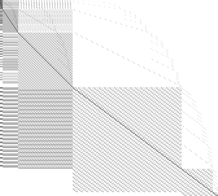
Figure 4. Grayscale image of the $756\times 840$ matrix from the non-minimal resolution of the AGR example with $n=6$, $d=5$, and $s=42$. Zero entries are white, entries with one term gray, and entries with two terms black. There are no entries with more than two terms.

6.2. Canonical Nodal Curves and Prym Canonical Nodal Curves

Our next two series of examples are randomly constructed canonical nodal curves (CNC) (see Tables 10 and 11) and Prym canonical nodal curves (PCNC) (see Tables 12 and 13) of genus $g$. For the series of CNC examples, we work over the finite field with 32,003 elements, whereas we consider the PCNC examples over fields of random positive characteristic between 10,000 and 30,000 as listed in the second column of Table 12.

Canonical curves are a widely studied topic, see, for example, [BS] for some references. Our interest in the minimal resolution of Prym canonical curves comes from [CEFS], where an analogue of Green’s conjecture for Prym curves was formulated. In terms of the resolutions computed with our method, both conjectures say that the degree zero parts of the syzygy matrices in the resolution have maximal rank. Computational results presented in [CEFS] indicate that the Prym-Green conjecture is very likely false for genus $g=8$ and $g=16$. It would be interesting to check experimentally whether $g=24$ is an exception as well. But our timings suggest that this is way out of reach even for our improved method. In fact, computing a resolution with LiftTree for the case $g=24$ would take, as a very rough estimate, about 100,000 years and 100 TB of memory.

Remark 6.1.

The non-minimal Betti numbers for the PCNC example with $g=14$ as computed with LiftTree are shown in Table 14. Note that the fifth differential $\phi_{5}$ contains a $1932\times 1932$ submatrix with constant entries. A black-and-white image of this submatrix is shown in Figure 5. Using specialized software such as FFLAS/FFPACK [DGP] which is easily available via Sage [S⁺14], checking that this matrix has full rank takes only 0.92 seconds. Thus, including the time to compute the non-minimal resolution (224.15 seconds, cf. Table 12), the verification of the Prym-Green conjecture for this case takes 225.07 seconds using our new method. If we only consider the time to compute the non-minimal resolution up to the fifth differential (129.87 seconds, cf. Table 15), this can be reduced to 130.79 seconds.

Remark 6.2.

For the PCNC example with $g=16$, the non-minimal Betti numbers as computed with LiftTree are shown in Table 6.2. Here, the sixth differential $\phi_{6}$ contains a $8910\times 8910$ submatrix with constant entries. Using FFLAS/FFPACK [DGP], it takes 55.24 seconds to check that the kernel of this submatrix is one-dimensional. Including the time to compute the non-minimal resolution up to the sixth differential (10,776.54 seconds, cf. Table 18), it thus takes little more than 3 hours to check that the verification of the Prym-Green conjecture based on nodal curves fails in this case. This is a substantial improvement of the running time for this problem in comparison to the time needed in [CEFS].

We also managed to compute the minimal Betti numbers for this example using the Singular command betti(), cf. Table 6.2. This computation took more than 37 hours, but it was run on a different compute server than the other examples due to the memory consumption exceeding 16 GB.

Finally, starting from the non-minimal resolution, we even succeeded to compute the syzygy scheme of the Prym-Green extra syzygy which prevents the minimal resolution of the curve from being pure, cf. Table 6.2. However, we found that in our example, this syzygy scheme is identical to the curve itself and does therefore not contribute any geometric information.

Table 10. Timings for the CNC examples (in sec.)

	Macaulay2	Singular
$g$	res	lres()	LiftTree	betti()	minres()
$5$	0	0	0	0	0
$6$	0.01	0	0	0	0
$7$	0.07	0.02	0.01	0	0
$8$	1.41	0.33	0.02	0	0.04
$9$	25.45	6.65	0.07	0.02	0.97
$10$	452.10	113.48	0.31	0.38	9.28
$11$	7,945.04	2,017.32	1.83	6.87	155.52
$12$	$-$	30,495.55	15.58	89.66	1,238.28
$13$	$-$	$-$	142.20	1,005.98	23,877.02
$14$	$-$	$-$	1,351.59	9,645.67	$-$
$15$	$-$	$-$	12,935.45	$-$	$-$

Table 11. Statistics for the non-minimal resolutions of the CNC examples

$g$	sec.	#Terms	#Mult.	#Add.	#Canc.	$Q_{\text{sparse}}$
$5$	0	258	466	226	0	3.583
$6$	0	1,411	2,161	831	0	2.520
$7$	0.01	6,038	8,104	2,323	3	1.677
$8$	0.02	22,343	27,123	5,453	18	1.075
$9$	0.07	75,054	84,804	11,319	63	0.669
$10$	0.31	235,179	253,212	21,434	169	0.408
$11$	1.83	699,758	730,490	37,790	380	0.244
$12$	15.58	1,998,583	2,047,201	62,944	758	0.144
$13$	142.20	5,522,774	5,593,998	100,053	1,393	0.084
$14$	1,351.59	14,854,811	14,949,653	152,971	2,382	0.049
$15$	12,935.45	39,056,118	39,164,376	226,312	3,866	0.028

Table 12. Timings for the PCNC examples (in sec.)

		Macaulay2	Singular
$g$	Char.	res	lres()	LiftTree	betti()	minres()
$6$	22,669	0	0	0	0	0
$7$	10,151	0.02	0.01	0	0	0
$8$	15,187	0.18	0.05	0.01	0	0.01
$9$	18,947	2.96	0.75	0.04	0	0.11
$10$	13,523	64.78	19.56	0.15	0.02	1.96
$11$	25,219	901.14	344.62	0.64	0.40	23.11
$12$	11,777	16,597.90	6,261.13	3.43	6.97	305.45
$13$	24,379	$-$	$-$	25.95	98.34	3,032.23
$14$	16,183	$-$	$-$	224.15	1,084.88	40,106.95
$15$	20,873	$-$	$-$	2,002.51	10,953.23	$-$
$16$	12,451	$-$	$-$	18,612.82	$-$	$-$

Table 13. Statistics for the non-minimal resolutions of the PCNC examples

$g$	sec.	#Terms	#Mult.	#Add.	#Canc.	$Q_{\text{sparse}}$
$6$	0	501	534	90	0	2.088
$7$	0	2,818	5,297	2,663	1	2.271
$8$	0.01	12,974	24,165	11,642	8	1.917
$9$	0.04	48,711	79,096	31,409	14	1.390
$10$	0.15	165,346	232,455	69,389	43	0.945
$11$	0.64	524,473	654,596	135,098	110	0.617
$12$	3.43	1,582,334	1,812,443	240,603	285	0.392
$13$	25.95	4,594,249	4,974,596	401,889	594	0.244
$14$	224.15	12,931,450	13,525,642	637,340	1,154	0.149
$15$	2,002.51	35,482,705	36,367,579	970,090	2,018	0.090
$16$	18,612.82	95,281,070	96,541,345	1,427,327	3,409	0.054

Table 14. Non-minimal Betti table for the PCNC example with $g=14$

	0	1	2	3	4	5	6	7	8	9	10	11
0:	1	-	-	-	-	-	-	-	-	-	-	-
1:	-	52	303	882	1596	1932	1602	903	332	72	7	-
2:	-	17	167	738	1932	3318	3906	3192	1788	657	143	14
total:	1	69	470	1620	3528	5250	5508	4095	2120	729	150	14

Table 15. Timings (in sec.) and statistics for the individual differentials $\phi_{i}$ in the non-minimal resolution of the PCNC example with $g=14$. Note that $\phi_{1}$ is given by the input ideal.

$i$	#Generators	#Terms	$Q_{\text{sparse}}$	Time	$\sim$ #Terms/sec.
1	69	3,064	44.406	$-$	$-$
2	470	50,208	1.548	0.54	92,978
3	1,620	371,814	0.488	6.25	59,490
4	3,528	1,290,516	0.226	37.98	33,979
5	5,250	2,639,132	0.142	85.10	31,012
6	5,508	3,436,908	0.119	70.07	49,050
7	4,095	2,917,668	0.129	21.21	137,561
8	2,120	1,593,830	0.184	2.72	585,967
9	729	530,548	0.343	0.25	2,122,192
10	150	94,488	0.864	0.02	4,724,400
11	14	6,338	3.018	0.01	(633,800)
2 to 11	23,484	12,931,450	0.149	224.15	57.691

Table 16. Non-minimal Betti table for the PCNC example with $g=16$

	0	1	2	3	4	5	6	7	8
11-11 0:	1	-	-	-	-	-	-	-	-
1:	-	75	539	1980	4653	7590	8910	7623	4730
2:	-	19	225	1221	4015	8910	14058	16170	13662
11-11 total:	1	94	764	3201	8668	16500	22968	23793	18392

	9	10	11	12	13
1-1	-	-	-	-	-
	2079	615	110	9	-
	8415	3685	1089	195	16
1-1	10494	4300	1199	204	16

Table 17. Minimal Betti table for the PCNC example with $g=16$

	0	1	2	3	4	5	6	7	8
11-11 0:	1	-	-	-	-	-	-	-	-
1:	-	75	520	1755	3432	3575	1	-	-
2:	-	-	-	-	-	1	6435	11440	11583
11-11 total:	1	75	520	1755	3432	3576	6436	11440	11583

	9	10	11	12	13
1-1	-	-	-	-	-
	-	-	-	-	-
	7800	3575	1080	195	16
1-1	7800	3575	1080	195	16

Table 18. Timings (in sec.) and statistics for the individual differentials $\phi_{i}$ in the non-minimal resolution of the PCNC example with $g=16$. Note that $\phi_{1}$ is given by the input ideal.

$i$	#Generators	#Terms	$Q_{\text{sparse}}$	Time	$\sim$ #Terms/sec.
1	94	4,706	50.064	$-$	$-$
2	764	96,185	1.339	1.75	54,963
3	3,201	881,460	0.360	51.64	17,069
4	8,668	3,884,192	0.140	669.57	5,801
5	16,500	10,428,510	0.073	3,332.74	3,129
6	22,968	18,632,465	0.049	6,720.84	2,772
7	23,793	23,035,835	0.042	5,663.46	4,067
8	18,392	19,959,667	0.046	1,897.21	10,521
9	10,494	12,027,377	0.062	260.48	46,174
10	4,300	4,889,758	0.108	14.46	338,158
11	1,199	1,257,155	0.244	0.59	2,130,771
12	204	178,565	0.730	0.08	2,232,063
13	16	9,901	3.033	0	$-$
2 to 13	110,499	95,281,070	0.054	18,612.82	5,119

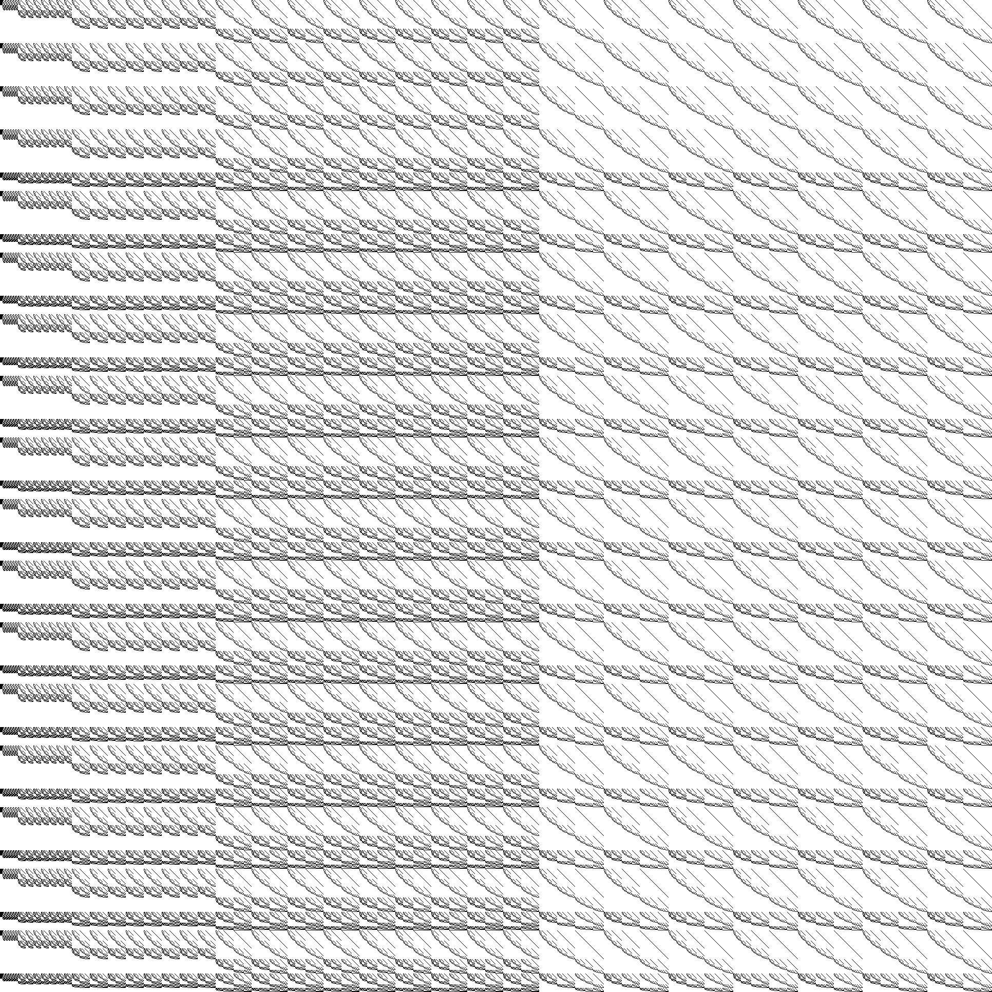
Figure 5. Black-and-white image of the $1932\times 1932$ constant submatrix from the non-minimal resolution of the PCNC example with $g=14$. Zero entries are white, constant entries are black. Note the somehow fractal structure.

7. Acknowledgements

We would like to thank Wolfram Decker for his steady encouragement during this project.

References

- [BS] Berkesch, C.; Schreyer, F.-O.: Syzygies, finite length modules, and random curves. arXiv:1403.0581 (2014). http://arxiv.org/abs/1403.0581
- [CEFS] Chiodo, A.; Eisenbud, D.; Farkas, G.; Schreyer, F.-O.: Syzygies of torsion bundles and the geometry of the level modular variety over . Invent. Math. 194.1 (2013), 73–118. http://arxiv.org/abs/1205.0661
- [DGP] Dumas, J.-G.; Giorgi, P.; Pernet, C.: Dense Linear Algebra over Word-Size Prime Fields: the FFLAS and FFPACK packages. ACM Trans. Math. Softw. 35.3 (2008), 1–42.
- [DGPS] Decker, W.; Greuel, G.-M.; Pfister, G.; Schönemann, H.: Singular 4-0-2 – A computer algebra system for polynomial computations (2014). http://www.singular.uni-kl.de
- [Eis95] Eisenbud, D.: Commutative algebra with a view toward algebraic geometry. Springer (1995).
- [GP] Greuel, G.-M.; Pfister, G.: A Singular Introduction to Commutative Algebra. Second edition, Springer (2007).
- [LS] La Scala, R.; Stillman, M.: Strategies for Computing Minimal Free Resolutions. J. Symb. Comput. 26.4 (1998), 409–431.
- [M2] Grayson, D.; Stillman, M.: Macaulay2, a software system for research in algebraic geometry (Version 1.7, 2014). http://www.math.uiuc.edu/Macaulay2/
- [M10] Motsak, O.: Graded Commutative Algebra and related Structures in Singular with applications. PhD thesis, Kaiserslautern (2010).
- [M14] Motsak, O.: schreyer.lib. A Singular 4-0-2 library for computing the Schreyer resolution of ideals and modules (2014).
- [OO] Oeding, L.; Ottaviani, G.: Eigenvectors of tensors and algorithms for Waring decomposition. J. Symb. Comput. 54 (2013), 9–35.
- [RS] Ranestad, K.; Schreyer, F.-O.: Varieties of sums of powers. J. Reine Angew. Math. 525 (2000), 147–181.
- [S80] Schreyer, F.-O.: Die Berechnung von Syzygien mit dem verallgemeinerten Weierstrasschen Divisionssatz. Diplomarbeit, Hamburg (1980).
- [S91] Schreyer, F.-O.: A Standard Basis Approach to Syzygies of Canonical Curves. J. Reine Angew. Math. 421 (1991), 83–123.
- [S+14] W. A. Stein et al.: Sage Mathematics Software (Version 6.4.1). The Sage Development Team (2014). http://www.sagemath.org