A Calibration of NICMOS Camera 2 for Low Count-Rates

Abstract

NICMOS 2 observations are crucial for constraining distances to most of the existing sample of $z>1$ SNe Ia. Unlike the conventional calibration programs, these observations involve long exposure times and low count rates. Reciprocity failure is known to exist in HgCdTe devices and a correction for this effect has already been implemented for high and medium count-rates. However observations at faint count-rates rely on extrapolations. Here instead, we provide a new zeropoint calibration directly applicable to faint sources. This is obtained via inter-calibration of NIC2 F110W/F160W with WFC3 in the low count-rate regime using $z\sim 1$ elliptical galaxies as tertiary calibrators. These objects have relatively simple near-IR SEDs, uniform colors, and their extended nature gives superior signal-to-noise at the same count rate than would stars. The use of extended objects also allows greater tolerances on PSF profiles. We find ST magnitude zeropoints (after the installation of the NICMOS cooling system, NCS) of 25.296$\pm 0.022$ for F110W and 25.803$\pm 0.023$ for F160W, both in agreement with the calibration extrapolated from count-rates $\gtrsim$ 1,000 times larger (25.262 and 25.799). Before the installation of the NCS, we find 24.843$\pm 0.025$ for F110W and 25.498$\pm 0.021$ for F160W, also in agreement with the high-count-rate calibration (24.815 and 25.470). We also check the standard bandpasses of WFC3 and NICMOS 2 using a range of stars and galaxies at different colors and find mild tension for WFC3, limiting the accuracy of the zeropoints. To avoid human bias, our cross-calibration was “blinded” in that the fitted zeropoint differences were hidden until the analysis was finalized.

1. Introduction

With the installation in 1997 of the Near Infrared Camera and Multi-Object Spectrometer (NICMOS) instrument, the Hubble Space Telescope (HST) first gained powerful near-IR capabilities (Thompson, 1992; Viana & et al., 2009). With low sky and diffraction-limited imaging, NICMOS was $\sim 10$ times faster at $J$ and $H$ point-source imaging than large ground-based telescopes with adaptive optics. Three cameras were available (NIC1, NIC2, and NIC3), each 256$\times$256 pixels, with pixel sizes of 0$\farcs$043 (NIC1), 0$\farcs$075 (NIC2), and 0$\farcs$2 (NIC3, which also had grism spectroscopy). The instrument was originally cooled to 61K by a block of nitrogen ice until lack of coolant stopped operations in 1999. In 2002, a servicing mission installed a cryocooler (the NICMOS Cooling System, NCS), allowing consumable-free operations at 77K.

NICMOS enabled the first probes of the earliest half of the expansion history of the universe (Riess et al., 2001, 2004, 2007; Suzuki et al., 2012; Rubin et al., 2013). Although precision ground-based $z>1$ SN measurements are possible (Tonry et al., 2003; Amanullah et al., 2010; Suzuki et al., 2012, Rubin et al., in prep), the required long exposure times with 10m-class telescopes make building a large sample expensive. NICMOS allowed for the measurement of precision colors (and thus, distances) for these distant SNe, sampling the rest-frame $B,V,R,$ or $I$ band, depending on filter and redshift. Even with the forthcoming Wide Field Camera 3 (WFC3)-observed SNe (Graur et al., 2013; Rodney et al., 2014) Postman et al., 2012, from the Cluster Lensing And Supernova search with Hubble, CLASH:, and Grogin et al., 2011; Koekemoer et al., 2011, the Cosmic Assembly Near-infrared Deep Extragalactic Legacy Survey, CANDELS:, NICMOS-observed SNe Ia will continue to make up the bulk of the $z>1$ sample.

NICMOS has proven to be a challenging instrument to calibrate. Bohlin et al. (2005) first found evidence of a count-rate non-linearity (CRNL) in NIC3 when extending spectrophotometric standards into the near IR. The Space Telescope Imaging Spectrograph (STIS) and NICMOS showed clear disagreement over the wavelength range in common (8,000 to 10,000Å), with NIC3 indicating a relative deficit of flux for fainter sources. Parameterizing the CRNL in terms of relative magnitude deficit per dex (factor of ten in count rate), NIC3 showed an increase of 0.06 mag/dex for count rates from $\sim 2$ to $\sim 3,000$/s ($\sim 0.18$ magnitudes over this $\sim 3$ dex range). Spectroscopy and imaging from the HST Advanced Camera for Surveys (ACS) agreed with STIS, pointing to NIC3 as the root of the problem. A comparison of three white dwarfs against models showed a strong wavelength dependence to the CRNL, with the CRNL consistent with zero longward of 16,000Å.

Mobasher & Riess (2005) first investigated this effect with ground-based data using both stars and galaxies. The stars had been observed in both F110W (a broad filter spanning $Y$ and $J$ centered at $1.1\mu$m) and F160W (similar to $H$, centered at $1.6\mu$m) in NIC2 and with ground-based $J$ and $H$ over the $J$ magnitude range 8-17 (Stephens et al., 2000). Their galaxies ranged in brightness down to the sky level, and were likewise observed in $J$ and $H$, but the NICMOS data came from NIC3 instead of NIC2. The star measurements showed no significant CRNL in either NIC2 band, with the F110W CRNL constrained to be a factor of at least 2-3 smaller than the NIC3 result from Bohlin et al. (2005). The galaxy measurements showed no significant CRNL until the measurements approached the sky level ($J\sim 23$) when the scatter became large and offsets $\sim 0.1$ magnitudes may have been indicated. The authors suggest that charge trapping may be responsible for the observed CRNL: exposures $\gtrsim 155$s (the persistence timescale), used to measure faint objects, may be able to fully fill the traps, resulting in a smaller CRNL.

de Jong et al. (2006) used exposures of star fields with and without counts enhanced by a flatfield lamp to directly measure the linearity of NIC1 and NIC2. Only count rates between $\sim 50$ and 2,000 counts per second were probed by this technique in NIC2 F110W, but the CRNL again seemed to be roughly constant in mag/dex over this range. Interestingly, the NIC2 F110W CRNL seemed to be the same size before and after the installation of the NCS and the associated change in temperature. In conflict with the exposure-time/charge-trap hypothesis, the observed CRNL is the same size whether the lamp-off data are taken after the lamp-on data (when the charge traps should be full) or before. In addition, Bohlin et al. (2006) checked the Bohlin et al. (2005) analysis using longer grism exposure times. They also find the same size NIC3 CRNL as with the shorter exposures, again at odds with the Mobasher & Riess (2005) results and a simple picture of charge-trapping. (We do however note that more-detailed models of charge-trapping do seem to fit lab-measured data, see Regan et al., 2012).

Taking the measurements from de Jong et al. (2006) and Bohlin et al. (2006), de Jong (2006) introduced a routine, rnlincor, that corrects the values in an image using an assumed power-law relation between the corrected and original values. The power-law is parameterized in units of mag/dex in the sense that

$$\mathrm{CR}_{\mathrm{estimated}} = \mathrm{CR}^{1/\{0.063\mathrm{[mag/dex}]/2.5+1\}}_{\mathrm{observed}}\hskip 14.45377pt\mathrm{for\ F110W}$$

$$\mathrm{CR}_{\mathrm{estimated}} = \mathrm{CR}^{1/\{0.029\mathrm{[mag/dex}]/2.5+1\}}_{\mathrm{observed}}\hskip 14.45377pt\mathrm{for\ F160W.}$$

The current convention is to then use the corrected count rate in combination with the zeropoint provided from bright standard stars. This procedure was used to calibrate the SNe in the Great Observatories Origins Deep Survey (GOODS) fields (Riess et al., 2007) and the Supernova Cosmology Project (SCP) high-redshift SNe in Nobili et al. (2009).

However, this solution was not an adequate calibration. The 0.006 mag/dex uncertainty on the NIC2 F110W CRNL translates into a $\sim 0.024$ mag uncertainty over the 4 dex range between the standard stars and high-redshift SNe. The effect of the strong wavelength-dependence of the CRNL over the F110W filter is hard to model for faint sources, as the amplifier glow is not at the same effective wavelength as the observations, and the dark current has no wavelength. As these sources are a significant fraction of the total background, this introduces $\sim 0.02$ magnitudes of uncertainty. It is also unclear even what effective count rate faint observations are taken at, as the amplifier glow may be constant, or produced in short bursts of high counts/second. We note that the Mobasher & Riess (2005) results could indicate that the NIC3 F110W power law breaks down at low count-rates and is wrong by $\sim 0.1$ magnitudes at low count-rates (possibly the sum of the above effects).

Given these issues, we were awarded 14 orbits to complete a precision calibration of NIC2 F110W at low count-rates, unlocking the full potential of the high-redshift SN Ia data. Suzuki et al. (2012) and Rubin et al. (2013) relied on a first-round SCP F110W calibration against a combination of ACS WFC and deep ground-based $J$ and $K$ data. This calibration indicated a zeropoint 0.055 magnitudes fainter (larger) than the extrapolation of the higher-count-rate calibrations, showing a weakening of the CRNL at low count-rates. Here, we derive an updated result, taking advantage of the similar WFC3 IR bandpasses. Given the larger number of archival WFC3 and NICMOS F160W observations now available, we are also able derive a result for F160W. Using fortuitous archival observations of mid-redshift galaxy clusters, we make the same measurement for pre-NCS observations.

Concurrently with our NIC2 investigations, Riess (2010) compared WFC3 IR starfield data against ACS F850LP and NIC2 F110W and F160W. With good precision (but only for count rates that are more than 10 times higher than high-redshift SN count rates) WFC3 IR showed a small power-law index CRNL ($\sim 6$ times smaller than for NIC2 F110W), that is approximately constant in mag/dex (as a function of count-rate) when compared against ACS and rnlincor-corrected NIC2 images. Similar WFC3 IR CRNL measurements were made by Riess & Petro (2010); Riess (2011) independently of NICMOS, so rnlincor seems to be accurate within the given uncertainties at these count rates.

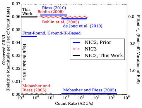
Figure 1.— Visual summary of the referenced NICMOS F110W calibration results and their approximate cosmological implications. Although this work is concerned with NIC2, we include NIC3 results (red dotted lines) to establish the level of uncertainty in the behavior of the count-rate non-linearity (although these results are not taken at quite the same effective wavelengths as the NIC2 results). Previous NIC2 results are color-coded in blue. Each line indicates the measured CRNL index and the range of count-rates it was measured at. The “first-round” result indicated a fainter NIC2 F110W zeropoint at low count-rates than the other calibrations, which we plot here assuming that the CRNL has a constant size for all count-rates. The results of our new calibration are consistent with the results of de Jong et al. (2006); Riess (2010) and are plotted in black. The cosmological results shown on the right axis are evaluated by fitting a time-varying $w_{0}$-$w_{a}$ model to the Union2.1 supernova compilation (Suzuki et al., 2012), and aligning $w_{a}=0$ with our calibration.

Figure 1 summarizes the measurements we reference. The size of the CRNL is shown (left axis), plotted against the range of count-rates over which it was measured. On the right axis, we use the Union2.1 supernova compilation, combined with BAO, CMB, and $H_{0}$ measurements (described in more detail in Suzuki et al., 2012) to convert from CRNL size to cosmological impact. For evaluating this impact, we use the $w_{0}$-$w_{a}$ model (Chevallier & Polarski, 2001; Linder, 2003) in which the equation of state parameter of dark energy smoothly varies with time as $w(a)=w_{0}+w_{a}(1-a)$. The high-redshift supernovae are particularly useful in constraining the time-variation, so we judge the impact using shifts in the best-fit $w_{a}$. A full cosmological analysis will be presented with other improvements in a future paper; for now, we compute the linear response of $w_{a}$ to the calibration and display that linear scale. The range of calibrations referenced here span $\sim 1.5$ in $w_{a}$. This is twice the size of all the other statistical and systematic uncertainties combined.

As the rnlincor power-law count-rate correction seems to be accurate at high count-rates, our strategy was to begin by correcting the NICMOS data for this relation. As all of our data (described below) encompasses a relatively narrow range in count-rates (centered around the count-rates of high-redshift SNe), we choose to derive an effective set of zeropoint differences between NIC2 and WFC3 (four, for F110W/F160W and pre-NCS/NCS). This strategy captures the relevant low-count-rate calibration, without necessitating the interpretation of data in other count-rate and exposure-time regimes.

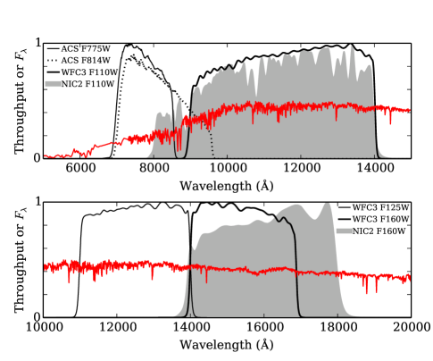
Figure 2.— The filter bandpasses referenced in this analysis, plotted against wavelength. Left to right in the top panel are the ACS WFC F775W filter (thin solid line), ACS WFC F814W filter (dotted line), the NIC2 F110W filter (filled), and the WFC3 F110W filter (thick solid line). Left to right in the bottom panel are the WFC3 F125W filter (thin solid line), the WFC3 F160W filter (thick solid line), and the NIC2 F160W filter (filled). For reference, an elliptical galaxy template redshifted to $z=1.2$ is overplotted in red. All normalizations are arbitrary.

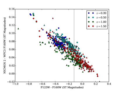
Figure 3.— Galaxy color-color relations for cross-calibrating F110W (top panel) and F160W (bottom panel), shown at a range of redshifts. Circular markers are stellar population synthesis models from Bruzual & Charlot (2003), while triangular markers are measurements of nearby galaxies (of all types) from Brown et al. (2013). The vertical gray lines indicate the median colors of the galaxies used in our calibration (for which these colors are available).

2. Data

Figure 2 presents the unnormalized HST bandpasses referenced in this analysis. The NIC2 and WFC3 F110W bandpasses are quite similar. The NIC2 F160W bandpass extends redder than the WFC3 F160W bandpass and requires a mild extrapolation outside the wavelength range of WFC3. In both cases, there is enough overlap that simple color-color relations can be used to cross-calibrate NICMOS and WFC3. For the F110W calibration, we use the F775W$-$F110W color as the abscissa, except when F775W is not available and we use F814W$-$F110W. For simplicity, we avoid F850LP data, as CCD scattering makes the PSF quite color-dependent (Sirianni et al., 1998). For the F160W calibration, we use the WFC3 F125W$-$F160W color as the abscissa, unless F125W is not available, in which case we use F814W$-$F160W or F110W$-$F160W. Example galaxy color-color relations at a range of redshifts are shown in Figure 3.

As illustrated in Figure 2, the elliptical galaxy templates used in this analysis are relatively flat in $f_{\lambda}$ inside the F110W and F160W bandpasses. We therefore choose to conduct our cross-calibration using Space Telescope (ST) magnitudes (magnitudes that are flat in $f_{\lambda}$, see Koornneef et al., 1986). Selecting a different magnitude system (e.g., AB or Vega, both of which use bluer references than ST) would have resulted in different calibration offsets and different correlations between calibration offsets and bandpass uncertainties. However, any cosmological results (using those cross-calibrations and covariance matrices) would be the same. ST magnitudes have the convenient advantage that the correlations can essentially be neglected.

We selected our calibration galaxies from ACS images, looking by eye for early-type morphologies and uniform colors. Each of the galaxies we selected showed stable colors when using photometry with different radius ranges (see Section A.2). Stacking the ACS data for each galaxy and removing an azimuthally symmetric galaxy model (one allowed to have ellipticity and an arbitrary spline radial profile) revealed spiral structure in some galaxies; these galaxies were removed from this analysis. For 14 out of 28 galaxies in the F160W calibration, we found archival WFC3 G141 spectroscopy (covering 11000Å to 17000Å), allowing us to examine the near-IR SED and determine the redshift. (Many redshifts also came from the literature, as summarized in Table 1.) For F110W, where the scatter of the color-color relation is smaller (and thus robust if a redshift is incorrect), we selected red-sequence galaxies (presented for the $z>1$ clusters in Meyers et al., 2012) from the galaxy clusters ISCS J1434.4+3426 (Brodwin et al., 2006), RDCS J1252.9-2927 (Rosati et al., 2004), XMMU J2235.3-2557 (Mullis et al., 2005), and Abell 1835 (Abell et al., 1989). Images of the selected galaxies are shown in Figure 4. Among our calibration galaxies are the host galaxies for the SNe SCP06C0, SCP06H5 (Suzuki et al., 2012), 05Lan, 04Tha, and 05Red (Riess et al., 2007). For the supernovae blended with their host galaxies, we used only the supernova-free reference images in this analysis.

Table 1Galaxies used in this measurement

Galaxy	RA	DEC	PIDs	Redshift	Redshift Source	Emission1	MW E($B-V$)
F110W, Post-NCS
F110W_01	193.22757	$-29.45461$	s, r, c	1.24	RDCS J1252.9$-$2927	$\cdots$	0.075
F110W_02	193.22703	$-29.45479$	s, r, c	1.24	RDCS J1252.9$-$2927	$\cdots$	0.075
F110W_03	193.22706	$-29.45644$	s, r, c	1.24	RDCS J1252.9$-$2927	$\cdots$	0.075
F110W_04	193.23039	$-29.45358$	s, r, c	1.24	RDCS J1252.9$-$2927	$\cdots$	0.075
F110W_05	193.22661	$-29.45602$	s, r, c	1.24	RDCS J1252.9$-$2927	$\cdots$	0.075
F110W_06	193.22575	$-29.45325$	s, r, c	1.24	RDCS J1252.9$-$2927	$\cdots$	0.075
F110W_07	193.22816	$-29.45401$	s, r, c	1.24	RDCS J1252.9$-$2927	$\cdots$	0.075
F110W_08	193.23039	$-29.45451$	s, r, c	1.24	RDCS J1252.9$-$2927	$\cdots$	0.075
F110W_09	193.22538	$-29.45500$	s, r, c	1.24	RDCS J1252.9$-$2927	$\cdots$	0.075
F110W_10	193.22505	$-29.45262$	s, r, c	1.24	RDCS J1252.9$-$2927	$\cdots$	0.075
F110W_11	193.22749	$-29.45127$	s, r, c	1.24	RDCS J1252.9$-$2927	$\cdots$	0.075
F110W_12	210.27313	$2.87484$	p, m	0.25	Abell 1835	$\cdots$	0.029
F110W_13	210.27098	$2.86989$	p, m	0.25	Abell 1835	$\cdots$	0.029
F110W_14	187.35722	$1.84900$	s, j	1.09	Santos et al. (2009); Dawson et al. (2009)	$\cdots$	0.022
F110W_15	218.62519	$34.44785$	s, j	1.24	ISCS J1434.4+3426	$\cdots$	0.018
F110W_16	218.62611	$34.44568$	s, j	1.24	ISCS J1434.4+3426	$\cdots$	0.018
F110W_17	218.62549	$34.44914$	s, j	1.23	Dawson et al. (2009)	$\cdots$	0.018
F110W_18	338.83679	$-25.96012$	s, r, j	1.39	XMMU J2235.3$-$2557	$\cdots$	0.021
F110W_19	338.83591	$-25.96062$	s, r, j	1.39	XMMU J2235.3$-$2557	$\cdots$	0.021
F110W_20	338.84198	$-25.95182$	s, r, j	1.39	XMMU J2235.3$-$2557	$\cdots$	0.021
F110W_21	338.83613	$-25.96230$	s, r, j	1.39	XMMU J2235.3$-$2557	$\cdots$	0.021
F110W_22	338.83593	$-25.96250$	s, r, j	1.39	XMMU J2235.3$-$2557	$\cdots$	0.021
F110W, Pre-NCS
F110W_61K_01	209.95569	$62.51310$	p, b, f	0.32	Fisher et al. (1998)	$\cdots$	0.019
F110W_61K_02	209.95828	$62.51344$	p, b, f	0.32	Fisher et al. (1998)	$\cdots$	0.019
F110W_61K_03	209.95741	$62.51513$	p, b, f	0.33	Fisher et al. (1998)	$\cdots$	0.019
F160W, Post-NCS
F160W_01	53.07643	$-27.84864$	i, t	1.54	v, Szokoly et al. (2004)	Y	0.007
F160W_02	53.06273	$-27.72659$	i, o	1.87	Balestra et al. (2010)	Y	0.009
F160W_03	53.06110	$-27.72709$	i, o	0.98	v, Le Fèvre et al. (2004)	Y	0.009
F160W_04	189.23715	$62.21721$	y, h, w	1.24	q, Barger et al. (2008)	Y	0.013
F160W_05	189.23575	$62.21603$	y, h, w	1.225	q	Y	0.013
F160W_06	189.22982	$62.21776$	y, h, w	0.95	q, Barger et al. (2008)	N	0.013
F160W_07	189.25714	$62.20662$	y, h, w	1.19	q, Barger et al. (2008)	Y	0.012
F160W_08	189.25511	$62.20382$	y, h, w	1.52	q, Cohen et al. (2000)	Y	0.012
F160W_09	189.03076	$62.16874$	w, g	0.64	q, Barger et al. (2008)	N	0.011
F160W_10	189.36618	$62.34293$	x, d	1.15	q, Wirth et al. (2004)	N	0.013
F160W_11	53.15855	$-27.69138$	i, o	0.67	v, Le Fèvre et al. (2004)	N	0.009
F160W_12	53.17661	$-27.69827$	i, o	0.68	Le Fèvre et al. (2004)	$\cdots$	0.009
F160W_13	53.16681	$-27.73859$	i, u	0.52	v, Le Fèvre et al. (2004)	N	0.008
F160W_14	53.19196	$-27.91250$	d, t	0.73	v, Vanzella et al. (2008)	N	0.008
F160W_15	53.18202	$-27.92357$	l, t	0.46	Le Fèvre et al. (2004)	$\cdots$	0.007
F160W_16	53.13239	$-27.81427$	h, u, t	0.77	v, Vanzella et al. (2008)	N	0.008
F160W_17	7.28240	$-0.93077$	k, n	0.23	Abazajian et al. (2009)	N2	0.021
F160W_18	137.86492	$5.85092$	z, e	0.78	Kneib et al. (2000)	$\cdots$	0.045
F160W_19	137.86643	$5.84706$	z, e	0.76	Kneib et al. (2000)	$\cdots$	0.045
F160W_20	137.86593	$5.84595$	z, e	0.76	Kneib et al. (2000)	$\cdots$	0.045
F160W_21	137.86604	$5.84474$	z, e	0.78	Kneib et al. (2000)	$\cdots$	0.045
F160W, Pre-NCS
F160W_61K_01	137.86492	$5.85092$	a, z	0.78	Kneib et al. (2000)	$\cdots$	0.045
F160W_61K_02	137.86643	$5.84706$	a, z	0.76	Kneib et al. (2000)	$\cdots$	0.045
F160W_61K_03	137.86593	$5.84595$	a, z	0.76	Kneib et al. (2000)	$\cdots$	0.045
F160W_61K_04	137.86604	$5.84474$	a, z	0.78	Kneib et al. (2000)	$\cdots$	0.045
F160W_61K_05	209.95617	$62.51328$	p, b	0.32	Fisher et al. (1998)	$\cdots$	0.019
F160W_61K_06	209.95872	$62.51361$	p, b	0.32	Fisher et al. (1998)	$\cdots$	0.019
F160W_61K_07	209.95785	$62.51530$	p, b	0.33	Fisher et al. (1998)	$\cdots$	0.019

Note. — Galaxies labeled “61K” are pre-NCS. The HST Program IDs are as follows: a = GO-7887, b = GO/DD-7941, c = GTO/ACS-9290, d = GO-9352, e = GO-9375, f = GTO/ACS-9717, g = GO-9856, h = GO-10189, i = GO-10258, j = GO-10496, k = GO-10886, l = GO-11135, m = GO-11143, n = GO-11202, o = GO/DD-11359, p = GO-11591, q = GO-11600, r = GO/DD-11799, s = GO/DD-12051, t = GO-12061, u = GO-12062, v = GO-12177, w = GO-12443, x = GO-12444, y = GO-12445, z = GO-12874.

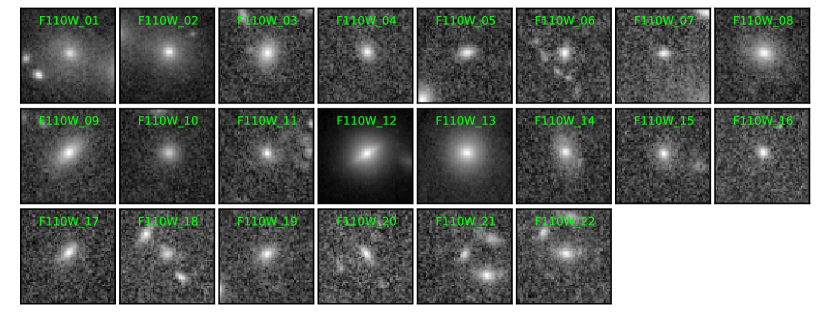
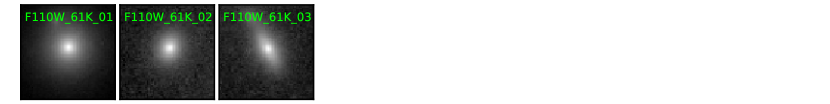
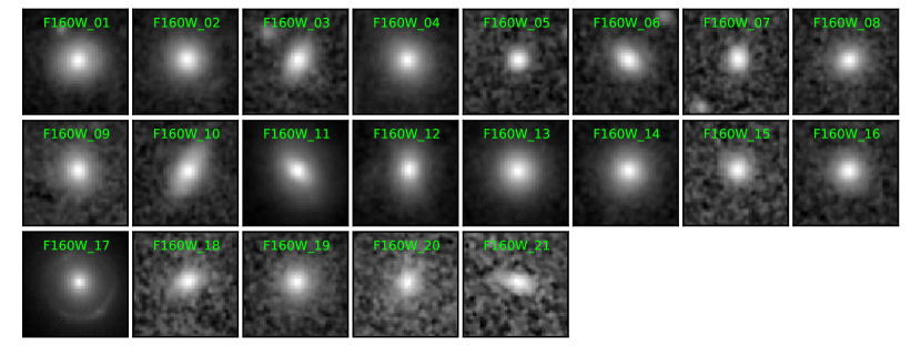
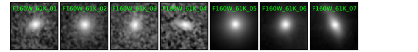
Figure 4.— 3″ by 3″ cutouts around each galaxy. The scaling is sinh^-1, so it approaches $\pm$logarithmic at large absolute fluxes, while approaching linear at small fluxes. This non-linear scaling brings out faint features, such as the Einstein ring around F160W_17.

3. Cross-Calibration Procedure

The ideal cross-calibration procedure would be to constrain the relative amplitude of the galaxy in each filter by directly modeling each pixel in each image, marginalizing out nuisance parameters for the underlying distribution of galaxy light on the sky, the exact alignment of the images, and the relative background levels. However, we instead selected cross-convolution for our analysis, as this approach limits the impact of systematics involved in understanding the PSF. The resulting increase in statistical uncertainty due to the convolution is limited by the convenient fact that the galaxies are significantly broader than the PSFs. (PSF systematics are suppressed to some extent when doing supernova photometry, as these systematics also affect measurements of standard stars, and only the differential measurement is important.)

We first resample the data onto the same pixel scale and orientation using astrodrizzle (Fruchter & et al., 2010). In short, this package resamples individual exposures into the same (distortion-free) frame, performs an initial robust image combination, rejects discrepant pixels (in the frames of the individual exposures), and then resamples the good pixels from each individual exposure to one final combined image. The name comes from the process of resampling, in which flux in the individual image is convolved with a kernel and then “drizzled” into a common undistorted frame.

Using PSFs derived from bright stars, we cross-convolve the images for each filter/instrument pair to be compared, giving the same PSF for both images (technical details in Appendix A.1). Once each pair of images has the same PSF, we centroid each galaxy, then compute fluxes in annuli around that centroid (A.2). We simultaneously fit for the true radial flux of the object (in the cross-convolved images), the relative sky level, and a scaling parameter. This scaling parameter (in units of magnitudes) represents the instrumental color of the galaxy in the pair of filters considered (instrumental color in that the zeropoints have not been taken into account). We then convert these instrumental colors to ST magnitude differences (A.3) using the Brown et al. (2013) galaxy templates (as a cross-check, we use templates from Bruzual & Charlot, 2003). Finally, we compute the average zeropoint offsets in A.4, including remaining uncertainty in the NIC2 bandpasses (see A.3.1) and uncertainty in the NIC2 CRNL.

To prevent inadvertent bias towards the expected results, our analysis was “blinded” (the zeropoints were kept hidden) until the analysis was complete. The order of the unblinding was as follows. First, we checked the code on bright standard stars, ensuring that the cross-convolution code matched the results of aperture photometry on the input images (cal/flt/flc, see below). This is a powerful test of the PSF models, as stars are much sharper than the calibration galaxies. Then, we unblinded the F160W results, as that band is less important for the cosmological results, and could have revealed gross problems with the analysis. (We made no analysis changes after unblinding the F160W.) Finally, we unblinded the F110W. We note that only the zeropoint offsets were kept hidden; the dispersions were never hidden, and provided one avenue of feedback for the proper drizzle settings (described in A.1) and the annuli-annuli correlations (described in Section B.5). The dispersion of the bright-star observations was a particularly useful diagnostic.

We evaluate the systematic uncertainties by changing assumptions one at a time (e.g., changing the minimum inner annuli radius of the photometry) and rerunning the analysis. To be conservative, the entire range (i.e., maximum $-$ minimum) is taken to be the $1\sigma$-size of that systematic. We sum these differences in quadrature. The full details of the uncertainty analysis are in Appendix B) while the contribution from each uncertainty is presented in Table 2. The composition of the total uncertainty depends on the calibration, but statistical uncertainty, PSF systematics, and the calibration of the galaxy templates share the bulk of it. WFC3 has its own calibration uncertainties, which we evaluate in B.8. These are currently comparable to the cross-calibration uncertainties, but may be reduced with future calibration programs.

Table 2Uncertainties present in the cross-calibrations.

Uncertainty	F110W	F160W	pre-NCS F110W	pre-NCS F160W
Statistical	10 mmag	6 mmag	8 mmag	8 mmag
Calibration of Color-Color	1 mmag	2 mmag	1 mmag	2 mmag
Encircled Energy Correction	2 mmag	2 mmag	2 mmag	2 mmag
PSF Shape	8 mmag	7 mmag	13 mmag	9 mmag
NICMOS Effective Bandpass	30Å	17Å	30Å	17Å
Annuli Correlations	5 mmag	1 mmag	10 mmag	1 mmag
Templates and Extinction	3 mmag	13 mmag	6 mmag	7 mmag
Total	14 mmag	17 mmag	19 mmag	14 mmag

4. Results

Table 3The results of our measurements.

Fit	NIC2 ST Zeropoint	NIC2 Low-Count-	STScI ST Zeropoint
	$-$ WFC3 ST Zeropoint	Rate ST Zeropoint
F110W
WFC3 Revised Bandpass	$-3.138$ mag	$25.296$	25.262
Standard Bandpass	$-3.145$ mag	$25.272$	25.262
Pre-NCS, WFC3 Revised Bandpass	$-3.591$ mag	$24.843$	24.815
Pre-NCS, Standard Bandpass	$-3.592$ mag	$24.825$	24.815
F160W
WFC3 Revised Bandpass	$-2.378$ mag	$25.803$	25.799
Standard Bandpass	$-2.376$ mag	$25.789$	25.799
Pre-NCS, WFC3 Revised Bandpass	$-2.683$ mag	$25.498$	25.470
Pre-NCS, Standard Bandpass	$-2.679$ mag	$25.487$	25.470

Note. — The bolded items are the recommended results. The difference in zeropoints is the quantity $k_{0}^{\mathrm{ST}}$, described in Section A.4.

Figure 5.— Diagram for the paths between the zeropoints discussed in this work. The “Blue/CALSPEC” zeropoints are referenced to CALSPEC calibration stars like solar analogs and Vega, which are bluer than the ST magnitude reference (flat in $f_{\lambda}$). The WFC3 CRNL measurements come from Riess (2010); Riess & Petro (2010); Riess (2011).

Table 3 presents our ST magnitude zeropoint differences for both the standard and revised WFC3 bandpasses (WFC3 bandpasses are discussed in A.3.2). We recommend the analyses highlighted in boldface type; any revisions to the WFC3 bandpasses can be interpolated from the pair of numbers from each result. Likewise, any updates to the understanding of the WFC3 zeropoints at low count-rates can be propagated through the results presented here into the NIC2 zeropoints. (The correlations between NICMOS and WFC3 zeropoints specified here should be taken into account in cosmological fits using the SN Ia Hubble diagram with both NIC2 and WFC3-observed SNe.)

Here, we illustrate the application of these results to the NIC2 zeropoints at low count-rates, applicable to any NIC2 cal files processed with the steps in A.1. We note that our zeropoints assume 1″-radius encircled energy corrections for F110W of 0.935 and 0.917 for F160W (we use PSF photometry for the supernova data, but the PSFs are normalized to these values), discussed further in A.1.

Figure 5 summarizes the paths for moving between the zeropoints we reference. Our calibration cross-calibrates WFC3 and NIC2, so we start with the WFC3 zeropoints. The observed Vega WFC3 F110W high-count-rate zeropoint (with our suggested bandpass revision) is 26.072. Accounting for the WFC3 CRNL, the zeropoint at low count-rates is 26.032. Converting to ST magnitude (using our bandpass revision) gives an ST zeropoint of 28.434. Applying our cross-calibration gives 25.296 for NIC2 ST. This same sequence was applied to both F110W and F160W; the resulting zeropoints are shown in second column of column of Table 3. For comparison, we take the NIC2 Vega STScI zeropoints, and convert to ST zeropoints using the low-count-rate conversions in Table 5. We follow this process, rather than using the STScI ST zeropoints, as the NIC2 Vega-to-ST conversion will depend on count-rate. These results are in the final column of Table 3. Our zeropoints range between 0.004 fainter (higher) for post-NCS F160W to 0.034 magnitudes fainter (higher) for post-NCS F110W, but show reasonable consistency. Other low-count-rate zeropoints (Vega or AB) can be computed using the low-count-rate offsets given in Table 5. We remind the reader that interpreting the photometric measurements should be done using a modified bandpass, as the CRNL preferentially affects blue wavelengths (discussed in A.3.1).

As a modest related result, we also note that the galaxy-galaxy scatter in the zeropoint estimates is a few percent. This limits spatial variation in the NIC2 CRNL to $\sim 10$ percent, at least on $\sim 1\arcsec$ scales.

5. Conclusions

This work presents a cross-calibration of the NIC2/WFC3 F110W and F160W zeropoints at the the low count-rates applicable to high-redshift SNe Ia observations. These measurements are in tension with both the Mobasher & Riess (2005) results (at least 0.1 mag tension), and some earlier unpublished SCP work (0.03 magnitudes tension). We note that this tension is not due to the version of calnica; we get essentially the same NICMOS magnitudes with the improved version 4.4.1 as with the older 4.1.1 that the pre-2008 results were run with (see the discussion of the improvements in Dahlen et al., 2008). Our results show no tension with the higher-count-rate zeropoint and CRNL measurements, with our results having smaller uncertainties at low count rates. A new “Union” compilation of SNe using this calibration will be presented in a future paper.

Appendix A Details of the Cross-Calibration

A.1. Data Processing

We started with the NICMOS cal files, flat-fielded files that have had cosmic rays rejected using the “up-the-ramp” multiple readouts. We processed each cal file first with the STSDAS task pedsky (Bushouse et al., 2000), to remove the variable quadrants seen in NICMOS data. We then ran rnlincor, to correct the images for the CRNL as measured at high count rates. After this processing, amplifier glow and other forms of spatially-variable background remained, so we ran the subtraction detailed in Hsiao et al. (2010). We used either the “low” or “high” background models, selecting the one that minimized the median absolute deviation of the image. We masked the erratic middle column, rather than attempting to recover the flux, as this data is far less important for our extended objects than for the SN data with which that work was concerned. Even after pedsky and our sky subtraction, the sky level in each image varies spatially. We thus fit for the residual sky under each galaxy, as shown in Equation A2.

We did no pre-drizzle processing of the WFC3 (flt, calibrated flat-fielded exposures) data or the ACS (flc, calibrated, flat-fielded, charge-transfer inefficiency-corrected exposures) data except using tweakreg to align the images. To prevent cosmic ray hits in the ACS images from being considered objects, we aligned L.A.Cosmic (van Dokkum, 2001) cleaned images. (Many of the ACS F775W visits had only one exposure per set of guide stars, so we chose to always align the input images (flt/flc), rather than stacking all of the data with a given set of guide stars and aligning the stacks.) To assist with the WFC3 alignment, we replaced each bad pixel with the median of the surrounding values. We then transferred the alignment to the original flt or flc images. For each instrument, we selected an optimal reference image based on depth and overlap with other images.

We used astrodrizzle to resample all data to a common pixel scale (0$\farcs$05, the native scale of ACS) and orientation (arbitrarily chosen to be North-up East-left) for cross-convolution. We selected a Gaussian kernel, with pixfrac=1 (the FWHM of the kernel in the input pixel scale). In testing, the kernel settings only had a mild impact on the dispersion of measured magnitudes. To prevent the loss of flux in the cores of bright stars, we weight each pixel in the drizzling by the exposure time of the image (this keeps the Poisson-dominated pixels from being deweighted). In our processing, we included some data quality (DQ) values that are non-zero, but still indicate a reliable flux measurement. Oddly, the post-NCS NICMOS data showed a difference in fluxes before and after astrodrizzle of 0.7%.

In order to cross-convolve the images, we must have an accurate PSF for each filter. Even if we had perfect model PSFs for the observed pixels, drizzling the data onto a new set of pixels will broaden the PSFs, making empirical PSFs a necessity. To derive NICMOS and WFC3 PSFs, we downloaded P330E data (a solar-analog calibration star with many observations), and derived a convolution kernel that matches Tiny Tim (Krist, 1993; Krist et al., 2011) PSFs to the drizzled P330E data. Although P330E is not as red as the calibration galaxies (and will thus have a slightly different PSF), it is the reddest standard for which a large amount of IR data exists. We discard any images that have non-zero DQ flags near the PSF core except the flags in the footnote. To derive ACS PSFs, we used bright, isolated stars selected from the fields, as there were not enough P330E images to derive PSFs.

These PSFs must be normalized. For this purpose, we normalize with a circular aperture of 1″-radius, which is large enough that the variation in encircled energy (EE) with object SED is a few mmag for all filters. It is also large enough to ensure that resampling the image does not affect the EE values. The normalization values for ACS F775W/F814W, taken from Sirianni et al. (2005), are 0.955. For NICMOS, we compute the EE values using Tiny Tim (version 7.5) with a range of SN, galaxy, and standard-star SEDs. We use 7x oversampling ($\sim$ 0$\farcs$01 per pixel), which matches the PSFs we use for SN photometry. (The EE values change coherently by $\sim$ 0.2% if we use 10x oversampling instead.) The average normalization values are 0.935 for F110W and 0.917 for F160W. For WFC3, we use the values from Hartig (2009) (to best match the STScI WFC3 calibration): F110W: 0.932, F125W: 0.927, and F160W: 0.915.

A.2. Fitting the Instrumental Colors, $k$

We centroid each galaxy in each drizzled stack by maximizing the flux inside a 0$\farcs$15 radius aperture (it makes virtually no difference if 0$\farcs$1 is used instead). (The signal-to-noises of these galaxies are high enough that this procedure is not significantly biased.) We then extract annular fluxes, $\mathbf{f}$, in 1-pixel-radius steps from 1 (or 3) to 10 (or 15) pixels, weighting each pixel by the fraction covered by the annulus. To obtain each color, we minimize the following expression:

$$\mathbf{r^{T}}\cdot C^{-1}\cdot\mathbf{r}+\log{|C|}\;.$$ (A1)

$\mathbf{r}$ is the residual from the model:

$$\mathbf{r}=\mathbf{f}-[10^{-0.4\;k}\;\mathbf{F}+s\;\mathbf{a}]\;,$$ (A2)

where $\mathbf{F}$ is the modeled flux of the galaxy in each annulus, $s$ is the modeled sky value, $\mathbf{a}$ is the area of each annulus, and $k$ is the modeled ratio of instrumental count-rates (measured in magnitudes). This is the count-rate ratio (as observed) between two filters and/or instruments, without correcting for the object SED or the zeropoints. There are arbitrary scaling and offset factors, which we handle by fixing $s$ and $k$ to zero for one filter. Although there is only one sky parameter, the symmetry of the annuli implies that the fit is insensitive to linear spatial variation of the sky (as well as a constant offset).

$C$ is the covariance matrix of the $\mathbf{f}$ values. The diagonal terms of $C$ are:

$$C_{ii}=\frac{10^{-0.4\;k}\;\mathbf{F}_{i}+s\;\mathbf{a}_{i}}{g\;t}+\mathbf{v}_{\mathrm{sky}_{i}}\;,$$ (A3)

where $g$ is the gain of the image (ADU/electron), $t$ is the exposure time, and $\mathbf{v}_{\mathrm{sky}}$ is the sky variance as determined empirically from object-free regions of the image. The first term is the Poisson uncertainty on the count-rates of the galaxy, while the second represents sky noise. As every image gets resampled by astrodrizzle, then convolved with another PSF, and then integrated in annuli (which share fractional pixels between neighboring annuli), there are large off-diagonal correlations. These correlations ($\rho_{ij}$) are also found empirically from object-free regions; we then set $C_{ij}=\rho_{ij}\sqrt{C_{ii}C_{jj}}$.

A.3. Fitting Zeropoint Offsets, $k^{\mathrm{ST}}$, for Each Galaxy

After obtaining the $k$ values (fitting out the $\mathbf{F}$ values and the $s$ values), we can fit the inter-calibrations. For the abscissa $k$ values, we scale out the following zeropoints: ACS F775W: 26.41699, ACS F814W: 26.79887, WFC3 F110W: 28.40001, WFC3 F125W: 27.9803, and WFC3 F160W: 28.1475 (these are the STScI zeropoints, with the WFC3 zeropoints shifted by 0.04 magnitudes for the WFC3 CRNL, see Section B.8). (The impact of the uncertainties on colors is discussed in B.3. Note that only differences in these zeropoints are meaningful, as they are used only to measure the color of each galaxy.) This gives us the abscissa ST magnitude color for each galaxy in the analysis. We fit linear relations to the color-color relations (see Figure 3 for typical relations), using templates with abscissa ST magnitudes within 0.25 of each observed galaxy. (This $\pm 0.25$ magnitude cut ensures that our results are not affected by the fact that the relations are not quite linear. This cut is large enough such that we always have several templates available to derive a local relation.) We subtract these relations from the ordinal $k$ values, producing estimates of the ST magnitude difference between NICMOS and WFC3, $k^{\mathrm{ST}}$.

We use the Brown et al. (2013) galaxy templates for our primary analysis. These templates are constructed using spectra and photometry of 129 nearby galaxies, with some interpolation using (mostly) stellar population synthesis models from Bruzual & Charlot (2003) (plus dust and PAH components). Although constructed from nearby galaxies, they match observed color-color relations at $z\sim 0.4$ (for details, see Brown et al., 2013), lending support to their use at higher redshift. As a cross-check, we use Bruzual & Charlot (2003) models, but do not use this as our primary analysis.

Synthesizing the color-color relations requires knowledge of the bandpasses, especially of NICMOS and WFC3 F110W and F160W (because of the shallow slopes of the color-color relations, the other bands are less important). Uncertainties in these bandpasses are described below.

A.3.1 NICMOS Effective Bandpass

The NICMOS CRNL depends strongly on wavelength, so the effective bandpasses of NICMOS will depend on count-rate, as illustrated in Figure 6. We measure excellent agreement between synthesized (using the 2014 March CALSPEC) and measured magnitudes among G191-B2B, GD153, GD71, GRW+70 5824, WD1657+343, P041C, P177D, P330E, SNAP-2, VB8 (the data here are saturated in F160W), 2M0036+18, and 2M0559-14 (F110W data only) using the synphot NIC2 bandpasses at high count-rates. This check limits any significant deviation from the standard bandpass to only the effects of the CRNL. There are no blue NIC2 medium or narrow-band filters, and no NIC2 grism, so we we cannot measure the change in NIC2 CRNL with wavelength. However, the CRNL (in mag/dex) is roughly linear with wavelength for NIC3, where it was measured in small wavelength bins using the grisms. We thus parameterize the effect on the NIC2 bandpasses using a function that is linear (in magnitudes) with respect to wavelength (i.e., an $\exp{(\lambda)}$ bandpass warping function). This function is constrained to be 0.063 magnitudes/dex at 11,000Å, and 0.029 magnitudes/dex at 16,000Å, matching the high-count-rate de Jong et al. (2006) measurements of the NIC2 CRNL in the F110W and F160W data, respectively. As we do not know the effective wavelength of amplifier glow (or how to treat dark current), we do not assume that this function should be evaluated with four dex (for the four dex separating the supernovae and standards). We instead parameterize the deviation from the high-count-rate bandpass in terms of the nuisance parameter $\beta$ (see Section A.4), which warps the bandpasses by $10^{-\beta\frac{2}{5}0.063}$ at 11,000Å and $10^{-\beta\frac{2}{5}0.029}$ at 16,000Å. Our standard analysis conservatively assumes a Gaussian prior of $2\pm 2$ on $\beta$, so that both four and zero are easily accommodated.

The sensitivity of NICMOS improved preferentially in the blue with the installation of the NCS. For the pre-NCS data, the bandpass must therefore be adjusted. Turning again to the NIC3 grism data (in G096L and G141L), we see that the pre/post-NCS sensitivity change is roughly linear with wavelength. As with the wavelength dependence of the CRNL, we fix the NIC2 slope with wavelength using the pre/post-NCS zeropoint change in the F110W and the F160W (0.45 and 0.33 magnitudes). This lets us handle pre-NCS data with the same bandpass model, just with the above prior on $\beta$ changed to $5.6\pm 2$.

Figure 6.— Plots of our model of the NIC2 F110W bandpass under different conditions, with arbitrary normalization. The blue line shows the bandpass taken from synphot. Observations of bright standard stars with a range of colors show consistency with this bandpass at those high count-rates. In red, we show the assumed bandpass two dex fainter ($\beta=2$). As described in Section A.3.1, the CRNL preferentially acts at blue wavelengths, shifting the bandpass effective wavelength to the red for lower count-rates. The pre-NCS NIC2 had worse sensitivity at blue wavelengths, giving a further effective-wavelength shift to the red shown in green ($\beta=5.6$).

A.3.2 WFC3 Effective Bandpass

Unlike NICMOS, the WFC3 CRNL is roughly independent of wavelength. Thus, establishing the WFC3 bandpasses at high count-rates is sufficient for all count-rates. (Although the galaxies in this analysis are close to zero ST color on average (flat in $f_{\lambda}$), knowledge of the WFC3 bandpasses is necessary to compute the ST magnitude zeropoint from the bluer standard stars.) As with NIC2, we check the observed and synthesized magnitudes of the standard stars G191-B2B, GD153, GD71, GRW+70 5824, WD1657+343, P041C, P177D, P330E, SNAP-2, and KF06T2 (for F160W, there is also data for VB8). These stars span a smaller range of colors than the stars observed with NIC2, but strongly indicate that shifts of the bandpasses to the red are necessary. Coincidentally, the effective-wavelength shifts needed for both filters are 60Å. We implement these shifts using the same smooth warping function used in Section A.3.1. As we only need the bandpass for converting between the Calspec-derived zeropoints and the ST magnitude zeropoints, the choice of functional form for the effective-wavelength shift will only have a small effect.

A.3.3 Synthesized High-Count-Rate Zeropoints

In Table 4, we present our Vega zeropoints derived from standard stars using 1″-radius aperture photometry. (Vega is close in color to the average standard used in this determination; these zeropoints can be transformed using Table 5.) The WFC3 bright zeropoints are fainter than the STScI zeropoints, as noted by Nordin et al. (2014) (who used PSF photometry). The WFC3 Vega zeropoints are almost independent of bandpass used, as the average color of the standard stars is not very dissimilar from Vega. Varying the photometry radius used can vary the zeropoints by several mmag, so these zeropoints are only tied to CALSPEC at the level of $\sim~{}0.01$ mag. The CALSPEC system itself also has uncertainty, so all of these zeropoints are most accurately defined with respect to other calibrations to that system. The NICMOS zeropoints show good agreement with their STScI counterparts, with some scatter. We note that the NICMOS bright zeropoints are only presented for comparison to the faint zeropoints, and do not enter our analysis (except to constrain the pre-NCS NIC2 bandpasses).

Table 4High-Count-Rate Vega Zeropoints

Bandpass	Observed Zeropoint	STScI Zeropoint
WFC3 F110W, Synphot	26.074	26.063
WFC3 F110W, Suggested Revision	26.072	$\cdots$
WFC3 F160W, Synphot	24.708	24.695
WFC3 F160W, Suggested Revision	24.708	$\cdots$
NICMOS F110W, Synphot	22.973	22.964
NICMOS F110W, Pre-NCS	22.500	22.500
NICMOS F160W, Synphot	22.144	22.153
NICMOS F160W, Pre-NCS	21.816	21.816

Note. — These zeropoints are computed using 1″-radius aperture photometry of bright standards with the March 2014 CALSPEC spectra. The proposed revisions of the WFC3 bandpasses have little effect on the Vega zeropoints, as the average color of the standards is not far from Vega. We find fainter (larger) zeropoints for WFC3, in accordance with Nordin et al. (2014). Our high-flux NICMOS zeropoints are presented for comparison only, and do not enter our analysis.

Table 5Synthesized Zeropoint Differences

Bandpass	Effective	ST $-$ Vega	AB $-$ Vega
	Wavelength	(Mag)	(Mag)
WFC3 F110W, Synphot	11797	2.3826	0.7647
WFC3 F110W, Suggested Revision	11857	2.4024	0.7728
WFC3 F160W, Synphot	15436	3.4978	1.2566
WFC3 F160W, Suggested Revision	15496	3.5131	1.2634
NICMOS F110W, Synphot	11575	2.2936	0.7328
NICMOS F110W, Suggested Low-CR	11605	2.3036	0.7366
NICMOS F110W, Pre-NCS and Low-CR	11659	2.3215	0.7434
NICMOS F160W, Synphot	16159	3.6474	1.3147
NICMOS F160W, Suggested Low-CR	16175	3.6515	1.3165
NICMOS F160W, Pre-NCS and Low-CR	16206	3.6588	1.3196

Note. — This table is intended to aid conversions among the different magnitude systems. We present the effective wavelength of each filter, computed for a source flat in $f_{\lambda}$. We also present ST $-$ Vega and AB $-$ Vega magnitude conversions. Each WFC3 result is presented with and without our proposed bandpass shift. We also present results using the NIC2 bandpasses at high-count rates, with the effects of the CRNL taken into account for low count-rates, and pre-NCS at low-count rates.

A.4. Fitting the Global Zeropoint Differences, $k_{0}^{\mathrm{ST}}$

Tests involving fitting a scale between images of the same galaxies in WFC3 data (with a range of spatial offsets and rotations) reveals a $\sim~{}0.03$ magnitude scatter. We take this as due to different pixel sampling in the undersampled images. The existence of this irreducible scatter implies that the statistical uncertainty is best judged (in part) using the observed dispersion of the scale factors about the mean. We must take into account residual uncorrected CRNL for both NIC2 and WFC3, as well as the partially known effective bandpass at these low count-rates. As we have enough data points to reliably estimate both calibration parameters and uncertainties using maximum likelihood, we minimize the following expression for each calibration:

$$\sum_{i}\frac{[k^{\mathrm{ST}}_{i}-(k_{0}^{\mathrm{ST}}+\alpha\;[M_{i}^{\mathrm{rnlincor}}-M_{\mathrm{mean\ SN}}^{\mathrm{rnlincor}}]+\beta\;C_{i}^{\mathrm{rnlincor}})]^{2}}{\sigma^{2}_{i}+\sigma_{\mathrm{int}}^{2}}+\sum_{i}\log(\sigma^{2}_{i}+\sigma_{\mathrm{int}}^{2})\;.$$ (A4)

$k_{i}^{\mathrm{ST}}$ is the ST magnitude NIC2$-$WFC3 difference measurement for each galaxy (with measurement uncertainty $\sigma^{2}_{i}$). $M_{i}^{\mathrm{rnlincor}}$ is the amount of non-linearity correction rnlincor applies to each galaxy. It is thus a surrogate count-rate measurement, with lower count-rates giving higher corrections. $M_{\mathrm{mean\ SN}}^{\mathrm{rnlincor}}$ is the mean rnlincor correction for the high-redshift SNe Ia near maximum, equal to 0.23 magnitudes in F110W and 0.10 magnitudes for F160W. $C_{i}^{\mathrm{rnlincor}}$ is the change in $k_{i}^{\mathrm{ST}}$ with respect to a change in count-rates by one dex due to the estimated wavelength-dependence of the CRNL (with respect to ST magnitude); it is thus a measure of the color of each galaxy. (Emission lines also play a role, but most of the variation is due to color.) We present our measurements of these parameters in Table 6.

The fit parameters are as follows. $k_{0}^{\mathrm{ST}}$ is the zeropoint offset defined for zero ST color and $M_{\mathrm{mean\ SN}}^{\mathrm{rnlincor}}$. $\alpha$ parameterizes any residual CRNL in either NIC2 or WFC3 (for simplicity, we assume that the WFC3 CRNL is proportional to the NIC2 CRNL). As described in Section A.3.1, $\beta$ is used to measure any deviation from the standard high-count-rate bandpasses. Finally, $\sigma_{\mathrm{int}}^{2}$ is a fit parameter representing irreducible variance (assumed to be the same for all galaxies in one band). The sum is usually over each galaxy. As there are not enough objects in the small NICMOS FoV to align separate NICMOS datasets, the sum ranges over these datasets, if more than one is present for a galaxy. As discussed in Section A.3.1, we take a prior of $2\pm 2$ on $\beta$ for the post-NCS NICMOS data, and $5.6\pm 2$ for the pre-NCS data. For the post-NCS data, we do not take any prior on $\alpha$, as we are testing for deviation from the predicted low-count-rate behavior. For the pre-NCS data (which uses many fewer objects), we assume that the WFC3 CRNL is 0.01 mag/dex, and the NICMOS CRNL is adequately corrected over this narrow range of count-rates (as it seems to have been in this count-rate range for the post-NCS data). $\alpha$ is thus fixed to 0.01 mag/dex / 0.063 mag/dex = 0.1587 for the pre-NCS F110W data and 0.01/0.029 = 0.3448 for the pre-NCS F160W data (recall that the 0.063 and 0.029 come from the de Jong et al., 2006, measurements of the NIC2 CRNL at high count-rates).

Illustrations of the fits are shown in Figure 7. We note that for the F110W data, it appears that the NIC2$-$WFC3 zeropoint gap narrows at very low count-rates (visible as higher points towards the right in the left panels). It may be that rnlincor over-corrects NIC2 F110W at these count-rates. Additional systematic uncertainty is likely called for when using rnlincor corrections greater than 0.25 magnitudes for NIC2 F110W.

There are three faint stars in the F110W data, allowing us to use them as a cross-check. For these, we use the Pickles (1998) stellar library for the color-color relation. As with the pre-NCS data, we fix $\alpha$, as we do not have enough objects over a large enough range of count-rates to reliably fit it. Large-aperture photometry on faint stars does not give high signal-to-noise, but we do find consistency with the galaxy results: $k_{0}^{\mathrm{ST}}=$ $-3.16\pm 0.04$ using the revised WFC3 bandpass.

As another cross-check, we fix $\alpha$ for the post-NCS data to investigate how fitting out uncorrected CRNL affects our results. The calibrations, using the modified WFC3 bandpasses, are only 4 mmag and 3 mmag (F110W and F160W, respectively) different. These tests indicate that our mean galaxy count-rate is close to the mean supernova count-rate. As a similar cross-check, we have objects spanning enough of a color range in F110W to unfix $\beta$ (although we now fix $\alpha$ for maximum statistical power). This results in a zeropoint difference of 10 mmag. Encouragingly, we find a $\beta$ measurement of $8.7\pm 6.2$, more consistent than not with the need to modify the bandpass at lower count rates.

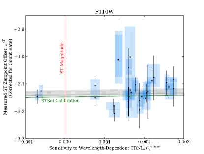
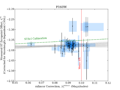
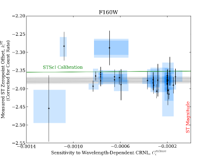
Figure 7.— The top panels present the galaxy measurements for F110W; the bottom panels show F160W. The $y$-axis is always $k_{i}^{\mathrm{ST}}$, the ST zeropoint difference observed between NIC2 and WFC3, computed using Brown et al. (2013) templates. The left panels show $k_{i}^{\mathrm{ST}}$ plotted against the size (in magnitudes) of the rnlincor NIC2 correction for the galaxy; this is a measure of relative galaxy surface brightness, with higher surface brightness galaxies towards the left. The right panels show $k_{i}^{\mathrm{ST}}$ plotted against $C_{i}^{\mathrm{rnlincor}}$, the effect of the wavelength dependence of the CRNL on $k_{i}^{\mathrm{ST}}$ as the count-rate changes by one dex. This is a measure of relative galaxy color, with redder galaxies to the right. The blue boxes (one for each galaxy) represent the range in results for different analyses (e.g., varying the outer photometry radius) for each point. The black points and error bars represent the mean for that galaxy, with the mean error bar including $\sigma_{\mathrm{int}}$. Each gray line is the fit for each variant (Section B). The green lines present the STScI NIC2 and WFC3 calibrations, with the WFC3 IR zeropoints moved 0.04 magnitudes brighter (smaller) to represent the uncorrected WFC3 CRNL. In the left plots, the green lines are not horizontal as the WFC3 CRNL has not been corrected, and thus the expected NIC2/WFC3 zeropoint difference changes with count rate. In the right plots, the green lines are not horizontal as they show the ($\beta=2$) NIC2 bandpass shift to the red representing the preferential loss of blue sensitivity due to the NIC2 CRNL (Section A.3.1).

Table 6Derived Galaxy Quantities

Galaxy	NICMOS CRNL	Abscissa Color	Abscissa Value	$k$	$k_{\mathrm{ST}}^{\beta=0}$	$C_{i}^{\mathrm{rnlincor}}$
F110W, Post-NCS
F110W_01	0.232	F775W $-$ F110W	1.273	$-3.205\pm 0.060$	$-3.158\pm 0.061$	0.00188
F110W_02	0.225	F775W $-$ F110W	1.303	$-3.196\pm 0.031$	$-3.148\pm 0.032$	0.00194
F110W_03	0.225	F775W $-$ F110W	1.355	$-3.204\pm 0.047$	$-3.154\pm 0.050$	0.00204
F110W_04	0.230	F775W $-$ F110W	1.144	$-3.082\pm 0.068$	$-3.040\pm 0.069$	0.00161
F110W_05	0.233	F775W $-$ F110W	1.171	$-3.173\pm 0.079$	$-3.130\pm 0.089$	0.00167
F110W_06	0.241	F775W $-$ F110W	1.160	$-3.160\pm 0.098$	$-3.118\pm 0.099$	0.00165
F110W_07	0.267	F775W $-$ F110W	1.016	$-3.031\pm 0.143$	$-2.995\pm 0.147$	0.00135
F110W_08	0.234	F775W $-$ F110W	1.448	$-3.140\pm 0.044$	$-3.087\pm 0.044$	0.00220
F110W_09	0.220	F775W $-$ F110W	1.369	$-3.188\pm 0.026$	$-3.138\pm 0.031$	0.00206
F110W_10	0.237	F775W $-$ F110W	1.140	$-3.203\pm 0.051$	$-3.161\pm 0.053$	0.00161
F110W_11	0.253	F775W $-$ F110W	1.145	$-3.179\pm 0.087$	$-3.137\pm 0.087$	0.00161
F110W_12	0.180	F814W $-$ F110W	-0.098	$-3.138\pm 0.005$	$-3.149\pm 0.007$	-0.00060
F110W_13	0.211	F814W $-$ F110W	-0.125	$-3.141\pm 0.016$	$-3.155\pm 0.016$	-0.00070
F110W_14	0.215	F775W $-$ F110W	1.070	$-3.218\pm 0.018$	$-3.187\pm 0.019$	0.00123
F110W_15	0.218	F775W $-$ F110W	0.766	$-3.139\pm 0.031$	$-3.113\pm 0.034$	0.00076
F110W_16	0.229	F775W $-$ F110W	0.966	$-3.242\pm 0.023$	$-3.207\pm 0.025$	0.00125
F110W_17	0.213	F775W $-$ F110W	1.240	$-3.157\pm 0.018$	$-3.112\pm 0.021$	0.00178
F110W_18	0.242	F775W $-$ F110W	1.464	$-3.169\pm 0.061$	$-3.112\pm 0.062$	0.00274
F110W_19	0.233	F775W $-$ F110W	1.410	$-3.167\pm 0.031$	$-3.112\pm 0.037$	0.00263
F110W_20	0.253	F775W $-$ F110W	1.235	$-3.117\pm 0.079$	$-3.068\pm 0.081$	0.00225
F110W_21	0.264	F775W $-$ F110W	1.172	$-3.160\pm 0.097$	$-3.113\pm 0.098$	0.00210
F110W_22	0.226	F775W $-$ F110W	1.379	$-3.152\pm 0.040$	$-3.098\pm 0.043$	0.00257
F110W, Pre-NCS
F110W_61K_01	0.169	F775W $-$ F110W	-0.065	$-3.599\pm 0.006$	$-3.609\pm 0.010$	-0.00045
F110W_61K_02	0.193	F775W $-$ F110W	-0.125	$-3.567\pm 0.013$	$-3.582\pm 0.016$	-0.00067
F110W_61K_03	0.191	F775W $-$ F110W	-0.076	$-3.599\pm 0.013$	$-3.610\pm 0.019$	-0.00050
F160W, Post-NCS
F160W_01	0.091	F125W $-$ F160W	-0.054	$-2.400\pm 0.019$	$-2.369\pm 0.020$	-0.00013
F160W_02	0.094	F125W $-$ F160W	-0.009	$-2.407\pm 0.016$	$-2.371\pm 0.016$	-0.00061
F160W_03	0.105	F125W $-$ F160W	-0.309	$-2.435\pm 0.041$	$-2.388\pm 0.042$	-0.00059
F160W_04	0.096	F125W $-$ F160W	-0.067	$-2.422\pm 0.016$	$-2.376\pm 0.018$	-0.00065
F160W_05	0.105	F125W $-$ F160W	-0.068	$-2.335\pm 0.045$	$-2.287\pm 0.046$	-0.00069
F160W_06	0.094	F125W $-$ F160W	-0.079	$-2.414\pm 0.017$	$-2.385\pm 0.019$	-0.00032
F160W_07	0.104	F125W $-$ F160W	-0.153	$-2.533\pm 0.091$	$-2.454\pm 0.093$	-0.00121
F160W_08	0.102	F125W $-$ F160W	-0.054	$-2.413\pm 0.029$	$-2.377\pm 0.029$	-0.00019
F160W_09	0.094	F125W $-$ F160W	-0.122	$-2.410\pm 0.022$	$-2.378\pm 0.022$	-0.00037
F160W_10	0.090	F125W $-$ F160W	-0.098	$-2.423\pm 0.009$	$-2.369\pm 0.011$	-0.00077
F160W_11	0.086	F125W $-$ F160W	-0.083	$-2.432\pm 0.009$	$-2.417\pm 0.011$	-0.00019
F160W_12	0.093	F125W $-$ F160W	-0.137	$-2.430\pm 0.016$	$-2.408\pm 0.016$	-0.00029
F160W_13	0.087	F125W $-$ F160W	-0.198	$-2.462\pm 0.010$	$-2.395\pm 0.010$	-0.00083
F160W_14	0.090	F125W $-$ F160W	-0.101	$-2.379\pm 0.013$	$-2.366\pm 0.013$	-0.00020
F160W_15	0.093	F125W $-$ F160W	-0.308	$-2.362\pm 0.038$	$-2.284\pm 0.040$	-0.00108
F160W_16	0.093	F125W $-$ F160W	-0.151	$-2.413\pm 0.021$	$-2.392\pm 0.022$	-0.00032
F160W_17	0.062	F814W $-$ F160W	-0.292	$-2.436\pm 0.005$	$-2.372\pm 0.007$	-0.00081
F160W_18	0.084	F125W $-$ F160W	-0.082	$-2.399\pm 0.028$	$-2.388\pm 0.029$	-0.00020
F160W_19	0.080	F125W $-$ F160W	-0.063	$-2.402\pm 0.019$	$-2.394\pm 0.020$	-0.00015
F160W_20	0.085	F125W $-$ F160W	-0.079	$-2.365\pm 0.038$	$-2.355\pm 0.038$	-0.00018
F160W_21	0.088	F125W $-$ F160W	-0.128	$-2.397\pm 0.043$	$-2.379\pm 0.046$	-0.00028
F160W, Pre-NCS
F160W_61K_01	0.082	F125W $-$ F160W	-0.082	$-2.677\pm 0.044$	$-2.666\pm 0.045$	-0.00020
F160W_61K_02	0.078	F125W $-$ F160W	-0.063	$-2.691\pm 0.029$	$-2.683\pm 0.030$	-0.00015
F160W_61K_03	0.084	F125W $-$ F160W	-0.079	$-2.666\pm 0.060$	$-2.656\pm 0.061$	-0.00018
F160W_61K_04	0.088	F125W $-$ F160W	-0.128	$-2.758\pm 0.074$	$-2.740\pm 0.078$	-0.00028
F160W_61K_05	0.066	F110W $-$ F160W	-0.167	$-2.758\pm 0.004$	$-2.710\pm 0.006$	-0.00065
F160W_61K_06	0.078	F110W $-$ F160W	-0.197	$-2.727\pm 0.008$	$-2.677\pm 0.009$	-0.00069
F160W_61K_07	0.077	F110W $-$ F160W	-0.172	$-2.752\pm 0.007$	$-2.704\pm 0.011$	-0.00067

Appendix B Details of the Uncertainty Analysis

B.1. Statistical Uncertainty

The statistical uncertainties in the fits of $k_{0}^{\mathrm{ST}}$ (Equation A4) are 10 mmag in F110W and 6 mmag in F160W (both post-NCS). As the likelihood is approximately Gaussian, these are computed using the Jacobian matrices with the covariance matrix of observations.

B.2. PSF Uncertainty

Our PSFs, derived from P330E, are not identical to the PSFs of the galaxies. This will lead to systematic mismatches between the photometry for different filters. We verify our PSFs by varying the inner radius used (either 1 or 3 pixels / 0$\farcs$05 or 0$\farcs$15). We also vary the outer radius used (10 or 15 pixels/ 0$\farcs$5 or 0$\farcs$75). The range spanned by these changes is 8 mmag in F110W and 2 mmag in F160W, which we take as a systematic uncertainty. We also try a fully empirical PSF (not relying on Tiny Tim as a first approximation). This makes a difference of only 1 mmag.

B.3. Impact of Other Zeropoints on the Color-Color Relations

The slopes of the color-color relations used to calibrate F110W are $\sim 0.03$ mag/mag (with modest variation for different redshifts, templates, and abscissa colors), see Figure 3. This implies that the $\sim 0.03$ mag uncertainties on the ACS/WFC3 relative calibration (including zeropoints, encircled-energy correction, and the WFC3 CRNL) will contribute 1 mmag to the uncertainty on the F110W calibration. For F160W, the slopes are $\sim 0.15$ mag/mag (again with modest variation), but the relative calibration uncertainties are smaller, as the abscissa colors generally both come from WFC3. We take a 2 mmag uncertainty for this relation.

B.4. Encircled Energy Correction

Our measurement is sensitive to the differential in encircled energy between NIC2 and WFC3. Future updates to the encircled energy corrections can be propagated into our results; for the moment, we take a 2 mmag uncertainty.

B.5. Annuli Correlations

The $C$ matrices that we empirically determine (Section A.2) have large off-diagonal correlations. These correlations are determined using object-free regions, and thus lack (smaller-scale) variations such as those caused by focus changes or sub-pixel position variations of sharp cores. As an approximate way to investigate the sensitivity to the ratio of small-scale to large-scale correlations in the $C$ matrices, we tried uniformly rescaling all of the off-diagonal elements by a range of values. These rescalings lower the dispersion in $k$ by more than a factor of two for stellar observations (these point-source observations show the largest response). There is little variation in the fitted zeropoint values or their error bars for a broad range of scale values, from 0.97 to 0 (where 0 results in an uncorrelated matrix). These rescalings have an effect of a few mmags on the post-NCS results (summarized in Table 2), which we take as systematic uncertainty.

B.6. Uncertainty in Galaxy SEDs

For the F160W bandpasses, the RMS residual from the color-color relation is 10 mmag, half of which we take as systematic uncertainty (to account for the fact that the average of our galaxies may not be the same as the average of the templates). Due to the similarities between the NIC2/WFC3 F110W bandpasses, the scatter in the color-color calibration for F110W is smaller (5 mmag), as shown in Figure 3. We again take half this as systematic uncertainty. Switching to the Bruzual & Charlot (2003) templates changes the zeropoints by $<1$ mmag and 12 mmag (F110W and F160W post-NCS, respectively). It is also possible that our galaxies have more (or less) dust than the nearby galaxies used in constructing the Brown et al. (2013) templates. Adding 0.1 magnitude of CCM reddening (Cardelli et al., 1989) to the templates (with $R_{V}=3.1$, so $A_{V}=0.31$) changes the zeropoints by $<1$ mmag and 2 mmag (F110W and F160W post-NCS, respectively). There is also uncertainty on the Milky Way foreground extinction for each galaxy, but these uncertainties affect our results at a trivial level.

B.7. AGN Variability

It is possible that some of our calibration galaxies have AGN, allowing them to change brightness in the time span between the NICMOS, ACS, and WFC3 observations. However, any large variability would flag the galaxy as unstable as we change the inner aperture size. Small variability is possible, but would increase $\sigma_{\mathrm{int}}$ in Equation A4 and so is already included in the statistical error bar.

B.8. WFC3 Uncertainties

Finally, we list WFC3 calibration uncertainties. As noted in Table 4, we find 0.01 magnitudes of tension with the STScI zeropoints. Our zeropoints also scatter by a few mmags depending on aperture radius, and show some tension between standard stars. Until these issues are resolved, we take a 0.01 uncertainty in the WFC3 bright zeropoints. Going from bright to faint zeropoints adds about 0.01 magnitudes of uncertainty for the WFC3 CRNL (Riess, 2010; Riess & Petro, 2010; Riess, 2011), and moves the effective zeropoints 0.04 magnitudes brighter (lower). To be conservative, we also take half of our proposed update of the WFC3 bandpasses (Section A.3.2 as uncertainty, giving 9 mmags in F110W and 7 mmags in F160W. In total, we estimate that the WFC3 low-count-rate ST zeropoints are $28.428\pm 0.017$ for F110W and $28.176\pm 0.016$ for F160W. Note that these zeropoints are tied to the CALSPEC system, which has uncertainties as well.

References

- Abazajian et al. (2009) Abazajian, K. N., Adelman-McCarthy, J. K., Agüeros, M. A., et al. 2009, ApJS, 182, 543
- Abell et al. (1989) Abell, G. O., Corwin, Jr., H. G., & Olowin, R. P. 1989, ApJS, 70, 1
- Amanullah et al. (2010) Amanullah, R., Lidman, C., Rubin, D., et al. 2010, ApJ, 716, 712
- Balestra et al. (2010) Balestra, I., Mainieri, V., Popesso, P., et al. 2010, A&A, 512, A12
- Barger et al. (2008) Barger, A. J., Cowie, L. L., & Wang, W.-H. 2008, ApJ, 689, 687
- Bohlin et al. (2005) Bohlin, R. C., Lindler, D. J., & Riess, A. 2005, Grism Sensitivities and Apparent Non-Linearity, Tech. rep.
- Bohlin et al. (2006) Bohlin, R. C., Riess, A., & de Jong, R. 2006, NICMOS Count Rate DependentNon-Linearity in G096 and G141, Tech. rep.
- Brodwin et al. (2006) Brodwin, M., Brown, M. J. I., Ashby, M. L. N., et al. 2006, ApJ, 651, 791
- Brown et al. (2013) Brown, M. J. I., Moustakas, J., Smith, J.-D. T., et al. 2013, ArXiv e-prints
- Bruzual & Charlot (2003) Bruzual, G., & Charlot, S. 2003, MNRAS, 344, 1000
- Bushouse et al. (2000) Bushouse, H., Dickinson, M., & van der Marel, R. P. 2000, in Astronomical Society of the Pacific Conference Series, Vol. 216, Astronomical Data Analysis Software and Systems IX, ed. N. Manset, C. Veillet, & D. Crabtree, 531
- Cardelli et al. (1989) Cardelli, J. A., Clayton, G. C., & Mathis, J. S. 1989, ApJ, 345, 245
- Chevallier & Polarski (2001) Chevallier, M., & Polarski, D. 2001, International Journal of Modern Physics D, 10, 213
- Cohen et al. (2000) Cohen, J. G., Hogg, D. W., Blandford, R., et al. 2000, ApJ, 538, 29
- Dahlen et al. (2008) Dahlen, T., McLaughlin, H., Laidler, V., et al. 2008, Improvements to Calnica, Tech. rep.
- Dawson et al. (2009) Dawson, K. S., Aldering, G., Amanullah, R., et al. 2009, AJ, 138, 1271
- de Jong (2006) de Jong, R. S. 2006, Correcting the NICMOS count-rate dependent non-linearity, Tech. rep.
- de Jong et al. (2006) de Jong, R. S., Bergeron, E., Riess, A., & Bohlin, R. 2006, NICMOS count-rate dependent nonlinearity tests using flatfield lamps, Tech. rep.
- Fisher et al. (1998) Fisher, D., Fabricant, D., Franx, M., & van Dokkum, P. 1998, ApJ, 498, 195
- Fruchter & et al. (2010) Fruchter, A. S., & et al. 2010, in 2010 Space Telescope Science Institute Calibration Workshop, p. 382-387, 382–387
- Graur et al. (2013) Graur, O., Rodney, S. A., Maoz, D., et al. 2013, ArXiv e-prints
- Grogin et al. (2011) Grogin, N. A., Kocevski, D. D., Faber, S. M., et al. 2011, ApJS, 197, 35
- Hartig (2009) Hartig, G. F. 2009, WFC3 SMOV Programs 11437/9: IR On-orbit PSF Evaluation, Tech. rep.
- Hsiao et al. (2010) Hsiao, E. Y., Suzuki, N., Ripoche, P., et al. 2010, in Hubble after SM4. Preparing JWST
- Kneib et al. (2000) Kneib, J.-P., Cohen, J. G., & Hjorth, J. 2000, ApJ, 544, L35
- Koekemoer et al. (2011) Koekemoer, A. M., Faber, S. M., Ferguson, H. C., et al. 2011, ApJS, 197, 36
- Koornneef et al. (1986) Koornneef, J., Bohlin, R., Buser, R., Horne, K., & Turnshek, D. 1986, Highlights of Astronomy, 7, 833
- Krist (1993) Krist, J. 1993, in Astronomical Society of the Pacific Conference Series, Vol. 52, Astronomical Data Analysis Software and Systems II, ed. R. J. Hanisch, R. J. V. Brissenden, & J. Barnes, 536
- Krist et al. (2011) Krist, J. E., Hook, R. N., & Stoehr, F. 2011, in Society of Photo-Optical Instrumentation Engineers (SPIE) Conference Series, Vol. 8127, Society of Photo-Optical Instrumentation Engineers (SPIE) Conference Series
- Le Fèvre et al. (2004) Le Fèvre, O., Vettolani, G., Paltani, S., et al. 2004, A&A, 428, 1043
- Linder (2003) Linder, E. V. 2003, Physical Review Letters, 90, 091301
- Meyers et al. (2012) Meyers, J., Aldering, G., Barbary, K., et al. 2012, ApJ, 750, 1
- Mobasher & Riess (2005) Mobasher, B., & Riess, A. 2005, A Test of Possible NICMOS Non-linearity, Tech. rep.
- Mullis et al. (2005) Mullis, C. R., Rosati, P., Lamer, G., et al. 2005, ApJ, 623, L85
- Nobili et al. (2009) Nobili, S., Fadeyev, V., Aldering, G., et al. 2009, ApJ, 700, 1415
- Nordin et al. (2014) Nordin, J., Rubin, D., Richard, J., et al. 2014, MNRAS, 440, 2742
- Pickles (1998) Pickles, A. J. 1998, PASP, 110, 863
- Postman et al. (2012) Postman, M., Coe, D., Benítez, N., et al. 2012, ApJS, 199, 25
- Regan et al. (2012) Regan, M., Bergeron, E., Lindsay, K., & Anderson, R. 2012, Count rate nonlinearity in near infrared detectors: inverse persistence
- Riess (2010) Riess, A. 2010, in Hubble after SM4. Preparing JWST
- Riess (2011) Riess, A. G. 2011, An Independent Determination of WFC3-IR Zeropoints and Count Rate Non-Linearity from 2MASS Asterisms, Tech. rep.
- Riess & Petro (2010) Riess, A. G., & Petro, L. 2010, Boosting Count-rates with Earth Limb Light and the WFC3/IR Count-rate Non-linearity, Tech. rep.
- Riess et al. (2001) Riess, A. G., Nugent, P. E., Gilliland, R. L., et al. 2001, ApJ, 560, 49
- Riess et al. (2004) Riess, A. G., Strolger, L.-G., Tonry, J., et al. 2004, ApJ, 607, 665
- Riess et al. (2007) Riess, A. G., Strolger, L.-G., Casertano, S., et al. 2007, ApJ, 659, 98
- Rodney et al. (2014) Rodney, S. A., Riess, A. G., Strolger, L.-G., et al. 2014, ArXiv e-prints
- Rosati et al. (2004) Rosati, P., Tozzi, P., Ettori, S., et al. 2004, AJ, 127, 230
- Rubin et al. (2013) Rubin, D., Knop, R. A., Rykoff, E., et al. 2013, ApJ, 763, 35
- Santos et al. (2009) Santos, J. S., Rosati, P., Gobat, R., et al. 2009, A&A, 501, 49
- Sirianni et al. (1998) Sirianni, M., Clampin, M., Hartig, G. F., et al. 1998, in Society of Photo-Optical Instrumentation Engineers (SPIE) Conference Series, Vol. 3355, Optical Astronomical Instrumentation, ed. S. D’Odorico, 608–612
- Sirianni et al. (2005) Sirianni, M., Jee, M. J., Benítez, N., et al. 2005, PASP, 117, 1049
- Stephens et al. (2000) Stephens, A. W., Frogel, J. A., Ortolani, S., et al. 2000, AJ, 119, 419
- Suzuki et al. (2012) Suzuki, N., Rubin, D., Lidman, C., et al. 2012, ApJ, 746, 85
- Szokoly et al. (2004) Szokoly, G. P., Bergeron, J., Hasinger, G., et al. 2004, ApJS, 155, 271
- Thompson (1992) Thompson, R. 1992, Space Sci. Rev., 61, 69
- Tonry et al. (2003) Tonry, J. L., Schmidt, B. P., Barris, B., et al. 2003, ApJ, 594, 1
- van Dokkum (2001) van Dokkum, P. G. 2001, PASP, 113, 1420
- Vanzella et al. (2008) Vanzella, E., Cristiani, S., Dickinson, M., et al. 2008, A&A, 478, 83
- Viana & et al. (2009) Viana, A., & et al. 2009, Near Infrared Camera and Multi-Object Spectrometer Instrument Handbook for Cycle 17 v. 11.0
- Wirth et al. (2004) Wirth, G. D., Willmer, C. N. A., Amico, P., et al. 2004, AJ, 127, 3121