Evolution in the Black Hole - Galaxy Scaling Relations and the Duty Cycle of Nuclear Activity in Star-Forming Galaxies

Abstract

We measure the location and evolutionary vectors of 69 Herschel-detected broad-line active galactic nuclei (BLAGNs) in the $M_{\rm{BH}}-M_{\ast}$ plane. BLAGNs are selected from the COSMOS and CDF-S fields, and span the redshift range $0.2\leq z<2.1$. Black-hole masses are calculated using archival spectroscopy and single-epoch virial mass estimators, and galaxy total stellar masses are calculated by fitting the spectral energy distribution (subtracting the BLAGN component). The mass-growth rates of both the black hole and galaxy are calculated using Chandra/XMM-Newton X-ray and Herschel far-infrared data, reliable measures of the BLAGN accretion and galaxy star formation rates, respectively. We use Monte Carlo simulations to account for biases in our sample, due to both selection limits and the steep slope of the massive end of the galaxy stellar-mass distribution. We find our sample is consistent with no evolution in the $M_{\rm{BH}}-M_{\ast}$ relation from $z\sim 2$ to $z\sim 0$. BLAGNs and their host galaxies which lie off the black hole mass $-$ galaxy total stellar mass relation tend to have evolutionary vectors anti-correlated with their mass ratios: that is, galaxies with over-massive (under-massive) black holes tend to have a low (high) ratio of the specific accretion rate to the specific star formation rate. We also use the measured growth rates to estimate the preferred AGN duty cycle for our galaxies to evolve most consistently onto the local $M_{\rm{BH}}-M_{\rm{Bul}}$ relation. Under reasonable assumptions of exponentially declining star formation histories, the data suggest a non-evolving (no more than a factor of a few) BLAGN duty cycle among star-forming galaxies of $\sim 10\%$ ($1\sigma$ range of $1-42\%$ at $z<1$ and $2-34\%$ at $z>1$).

1. Introduction

As the most luminous persistent sources in the Universe, active galactic nuclei (AGNs), which are powered by the mass accretion of super-massive black holes (SMBHs), are widely believed to play important roles in the formation and evolution of typical massive galaxies (for a recent review, see Kormendy & Ho, 2013). Indeed, over the past sixteen years, many studies have revealed that there are tight correlations between SMBHs and the physical properties of host galaxies (e.g., Magorrian et al., 1998; Ferrarese & Merritt, 2000; Gebhardt et al., 2000; Tremaine et al., 2002; Marconi & Hunt, 2003; Häring & Rix, 2004; Gültekin et al., 2009). For example, the SMBH mass, $M_{\rm BH}$, correlates well with the stellar mass of the bulge, $M_{\rm Bul}$. The intrinsic scatter of the $M_{\rm BH}-M_{\rm Bul}$ relation is found to be $\sim 0.3\ \rm{dex}$. Such a tight correlation might be explained by AGN feedback (e.g., Silk & Rees, 1998; King, 2003; Fabian, 2012). In this scenario, winds or jets launched from the accretion disk of the SMBH heat the interstellar medium (ISM) or clear the ISM out of the host galaxy. Star formation is therefore quenched due to the lack of cold gas. Such a coupled AGN triggering and feedback-regulated star formation could be responsible for the $M_{\rm BH}-M_{\rm Bul}$ relation (see, e.g., Di Matteo et al., 2005; Hopkins et al., 2006). On the other hand, a non-causal origin of the $M_{\rm BH}-M_{\rm Bul}$ relation has also been proposed by Jahnke & Macciò (2011) (see also Peng, 2007). In this scenario, $M_{\rm BH}$ and $M_{\rm Bul}$ are not initially correlated. The $M_{\rm BH}-M_{\rm Bul}$ relation is established simply by galaxy-galaxy mergers via the central limit theorem. Direct observational measurement of the evolution of the $M_{\rm BH}-M_{\rm Bul}$ relation is crucial to investigate the formation and co-growth of SMBHs and their hosts.

Observationally, the evolution of the $M_{\rm BH}-M_{\rm Bul}$ relation is still a controversial topic (e.g., Peng et al., 2006; Treu et al., 2007; Jahnke et al., 2009; Merloni et al., 2010; Bennert et al., 2011; Schramm & Silverman, 2013). Moreover, at high redshift (e.g., $z\sim 1$), it is very difficult to separate the bulge from the total stellar mass. Instead, most works explore the $M_{\rm BH}-M_{\ast}$ relation, where $M_{\ast}$ is the galaxy total stellar mass. For instance, Jahnke et al. (2009) find that at $z\sim 1.4$ the $M_{\rm BH}-M_{\ast}$ relation is consistent with the local $M_{\rm BH}-M_{\rm Bul}$ relation. Note that the host galaxies of the local sample of Häring & Rix (2004) (hereafter HR04) are bulge dominated (i.e., $M_{\rm Bul}\sim M_{\ast}$). Therefore, the Jahnke et al. (2009) result suggests little evolution of the $M_{\rm BH}-M_{\ast}$ relation to $z\sim 1.4$. On the other hand, the hosts of the Jahnke et al. (2009) sample have substantial disks (i.e., $M_{\rm{Bul}}<M_{\ast}$). That is, the $M_{\rm BH}-M_{\rm Bul}$ relation does evolve as a function of redshift. Making the local $M_{\rm BH}-M_{\rm Bul}$ relation then, as pointed out by Jahnke et al. (2009), requires a redistribution of stellar mass from disks into bulges in AGN host-galaxies. Recently, the work of Schramm & Silverman (2013) with a larger and less-biased sample also supported the results of Jahnke et al. (2009). On the other hand, Merloni et al. (2010) compiled a broad emission-line AGN (BLAGN) sample with well-measured multi-band photometry from the COSMOS survey. With this sample, they find that even the $M_{\rm BH}-M_{\ast}$ relation evolves (at $5\sigma$ significance level) over cosmic time (i.e., the SMBH is over-massive at high redshifts; see also Bennert et al., 2011). However, as pointed out by Lauer et al. (2007), high-redshift samples are generally selected by AGN activity (which depends on $M_{\rm BH}$) and suffer from Eddington bias. The physical reasons are: (1) there is intrinsic scatter in the $M_{\rm BH}-M_{\rm Bul}$ or $M_{\rm BH}-M_{\ast}$ relation; (2) the galaxy stellar mass function is bottom heavy (i.e., the number density of galaxies steeply decreases to higher stellar mass). Hence, for these high-redshift samples, an AGN with given $M_{\rm BH}$ is more likely to be found in less massive galaxies, resulting in an apparent evolution of the $M_{\rm{BH}}-M_{\rm{Bul}}$ or $M_{\rm BH}-M_{\ast}$ relation (also see Section 4.1). This bias increases with redshift as at high redshifts we often only have access to very luminous AGNs (very massive SMBHs). Additionally, $M_{\rm BH}$ estimation itself is also biased for these high-redshift samples (Shen & Kelly, 2010). The reasons are similar: (1) $M_{\rm BH}$ is estimated from AGN luminosity which also has intrinsic scatter; (2) the AGN luminosity function is also bottom heavy. Note that the sample of Schramm & Silverman (2013) consists of mostly lower luminosity AGNs and hence suffers less bias than Merloni et al. (2010). Bias corrections must be made to compare the high-redshift $M_{\rm BH}-M_{\ast}$ relation with the local one (for a more recent discussion on this topic, see, e.g., Schulze & Wisotzki, 2014).

In addition to measuring the $M_{\rm BH}-M_{\ast}$ relation at high redshift, it is also valuable to study its instantaneous evolution; i.e., the SMBH and galaxy stellar mass growth rates. Especially, will future SMBH and galaxy mass increases help establish/maintain the $M_{\rm BH}-M_{\ast}$ relation? This question has been indirectly investigated. For example, many works explored the possible connection between star formation rates (SFRs) and AGN luminosities (e.g., Rafferty et al., 2011; Mullaney et al., 2012; Rosario et al., 2012, 2013a, 2013b; Chen et al., 2013, and also see Alexander & Hickox 2012 for a review). However, as pointed out by Hickox et al. (2014), AGN variability can dilute the intrinsic correlation between star formation and AGN activity. Therefore, this connection is expected to be observed only in an average sense, as individual galaxies will tend to show a much weaker (or absent) correlation. The average SMBH accretion rate traces the average SFR so well that the local $M_{\rm BH}-M_{\ast}$ relation can be established.

Simultaneously exploring both the $M_{\rm BH}-M_{\ast}$ relation at high redshifts and its instantaneous evolution is even more valuable but is challenging. Merloni et al. (2010) explore this issue by measuring $M_{\rm BH}$, $M_{\ast}$, and their growth rates. They find that star formation and AGN activity can actually help reduce the scatter of the $M_{\rm BH}-M_{\ast}$ relation. However, the SFR in their work is estimated by fitting a stellar population synthesis model to the optical-to-NIR spectral energy distribution (SED) which has an uncertainty of $\sim 0.7\ \rm{dex}$. A more accurate determination of SFR (e.g., with Herschel observations) could better elucidate the coupled growth of AGNs and their host galaxies.

In this work, we uniquely explore the $M_{\rm{BH}}-M_{\ast}$ relation and its evolution, accounting for biases and using robust and uncontaminated estimates of SMBH growth and galaxy star formation rate. In Section 2, we describe our sample in detail. In Section 3, we describe our methods for estimating $M_{\rm BH}$, $M_{\ast}$, $\dot{M}$, and $\rm SFR$. In Section 4 we discuss selection biases and present our results. In Section 6, we discuss implications of our results. Finally, we summarize our main results and outline the possible future improvements in Section 7. Throughout this work we adopt a flat $\Lambda$CDM cosmology with $H_{0}=70\ \rm{km\ s^{-1}\ Mpc^{-1}}$, $\Omega_{\rm{M}}=0.3$ and $\Omega_{\Lambda}=0.7$.

2. Sample Construction

The $2$-$\rm{deg}^{2}$ Cosmic Evolution Survey (COSMOS, Scoville et al., 2007) and $464.5$-$\rm{arcmin}^{2}$ Chandra Deep Field-South survey (CDF-S; e.g., Luo et al., 2008, 2010; Xue et al., 2011) both have well-calibrated multi-band photometry (from the X-ray to radio bands) and high-quality spectroscopic coverage. Hence, we selected our sample from the COSMOS and CDF-S fields. First, we selected BLAGNs based on X-ray detection of AGN activity (for the advantages of using X-ray selection, see Brandt & Alexander, 2010) and subsequent optical spectroscopic identification of broad emission lines (with coverage of either $\rm{H}\beta$ or Mg ii). Second, we cross-matched our BLAGNs with the Herschel PEP (Lutz et al., 2011) (for the CDF-S field, we also used the GOODS–Herschel catalogs, see Elbaz et al., 2011; Magnelli et al., 2013) and HerMES (Oliver et al., 2012; Wang et al., 2013) catalogs. Third, the new sample was cross-matched with existing multi-band photometric catalogs to build the final sample. In the following subsections, we discuss our sample selection in detail (see also Table 1).

2.1. COSMOS Field BLAGNs

The $2$-$\rm{deg}^{2}$ COSMOS field has been surveyed in the X-ray by XMM-Newton (Cappelluti et al., 2009; Brusa et al., 2010) and partially (0.9 $\rm{deg}^{2}$) by Chandra (Elvis et al., 2009; Civano et al., 2012). We first selected all $z<2.4$ BLAGNs (ensuring the coverage of either $\rm{H}\beta$ or Mg ii) from the public COSMOS spectroscopy (Lilly et al., 2007; Trump et al., 2009a). Our BLAGNs have public Magellan/IMACS (Trump et al., 2009a), SDSS (York et al., 2000), or VLT/VIMOS (zCOSMOS; Lilly et al., 2007) spectroscopic data which allow us to estimate $M_{\rm BH}$ via the single-epoch approach (see also Section 3.1). The Magellan/IMACS spectroscopy is limited by $i_{\rm AB}<22.5$ (Trump et al., 2009a). For consistency and ease of modeling the observational biases, we impose the same $i_{\rm AB}<22.5$ limit for the combined COSMOS and CDF-S sample. We then cross matched them with X-ray catalogs to get the corresponding (rest-frame) $2-10\ \rm{keV}$ luminosity. For X-ray observations, we prefer Chandra over XMM-Newton and hard band over soft band (i.e., the Chandra hard band has the highest priority, and the XMM-Newton soft band has the lowest priority). As pointed out by Trump et al. (2009a, 2011) and will be shown in Figure 3, our AGN selection is limited by the $i_{\rm AB}<22.5$ criteria and not the X-ray sensitivity (whether XMM-Newton or Chandra).

To get a robust estimate of SFR, we cross-matched our BLAGN sample with the Herschel PEP ($100\ \rm{\mu m}$ and $160\ \rm{\mu m}$) and HerMES ($250\ \rm{\mu m}$) catalogs. Note that for the HerMES catalog the SPIRE/Herschel observations have a large point-spread function. We followed Chen et al. (2013) and chose a maximum matching radius of $5^{{}^{\prime\prime}}$. The Herschel PEP catalogs have improved astrometry because sources were extracted using Spitzer/MIPS $24\ \rm{\mu m}$ priors, and so we used a maximum matching radius of $2^{{}^{\prime\prime}}$. As for multi-band photometry, we used the COSMOS Photometric Redshift Catalog Fall 2008 (Ilbert et al., 2009) to get the optical-to-NIR broad-band photometry information ($B$, $V$, $g$, $r$, $z$ of Subaru; $u$, $i$, $Ks$ of CFHT; and $J$ of UKIRT) for the selected sources (see also Capak et al., 2007; McCracken et al., 2010). We also included four Spitzer/IRAC channels (Sanders et al., 2007) and GALEX/Near UV data when available. Zero-point corrections suggested in Ilbert et al. (2009) were applied. The Galactic extinction was also corrected using the Galactic extinction map of Schlegel et al. (1998). Note that for the optical-to-NIR bands, the Galactic extinction corrections are already included in the catalog.

2.2. CDF-S Field BLAGNs

The $464.5$-$\rm{arcmin}^{2}$ CDF-S field is covered by the deepest X-ray survey, with $4$ Ms of Chandra coverage (Xue et al., 2011). We selected BLAGNs by cross-matching the 4 Ms CDF-S catalog with the optical spectroscopy of Szokoly et al. (2004). Similar to the COSMOS sources, we only selected BLAGNs (with $i_{\rm AB}<22.5$) whose host galaxies are also detected by the Herschel PEP or HerMES (the cross-matching criteria is the same as that of COSMOS BLAGNs). As for multi-band photometry, we used the MUSYC 32-band (including $U$, $U38$, $B$, $V$, $R$, $I$, $z$, $J$, $H$, $K$ bands; 18 Subaru medium bands; and four Spizter/IRAC channels) catalog (Cardamone et al., 2010, and references therein). The Galactic extinction and zero-point corrections suggested in Cardamone et al. (2010) were adopted.

2.3. Total BLAGNs

Based on the above criteria, we started with a total number of 251 X-ray BLAGNs at $z<2.4$ (ensuring coverage of either $\rm{H}\beta$ or Mg ii), with 221 from the COSMOS field and 30 from the CDF-S field. When cross-matched with the Herschel catalogs, 96 sources were left (85 from the COSMOS field; 11 from the CDF-S field). 69 of these 96 sources have high-quality spectroscopic observations and robust FIR detections which enable us to measure $M_{\rm BH}$, $M_{\ast}$, $\dot{M}$, and SFR, reliably. For the other 27 sources, either the spectroscopic data (nine objects) or the FIR observations (18 objects) are not sufficient for a reliable measurement of $M_{\rm BH}$ or SFR (see Sections 3.1 & 3.4). Note that due to the Herschel sensitivity, $\sim 2/3$ of BLAGNs are undetected. We will consider the bias introduced by the Herschel sensitivity in Section 4.1.

For the 69 sources in our sample, 62 are from the COSMOS field and seven are from the CDF-S field. Note that their spectra are flux calibrated. We compared the physical properties (Section 3) of these seven CDF-S sources with the COSMOS sources (using the Mann-Whitney U test) and found no statistical difference (i.e., the null probability $p>0.05$).

3. Measuring Properties of AGNs and Their Host Galaxies

3.1. Black-Hole Mass Estimation

We adopted single-epoch virial SMBH mass estimators to estimate SMBH masses. More specifically, H$\beta$ or Mg ii line estimators were used depending on the redshift. These SMBH mass estimators use the correlation between the radius of the broad line region (BLR), $R_{\rm BLR}$, and the continuum luminosity, $\lambda L_{\lambda}$, $R_{\rm{BLR}}\propto(\lambda L_{\lambda})^{0.5}$, revealed by reverberation mapping observations of local AGNs (Bentz et al., 2006; Kaspi et al., 2007). If the BLR is virialized, then the SMBH mass can be estimated by $M_{\rm{BH}}=fR_{\rm{BLR}}v^{2}_{\rm{FWHM}}$, where $v_{\rm{FWHM}}$ is the full width at half maximum of the broad emission line and $f$ is related to the BLR geometry (calibrated from dynamical estimates of $M_{\rm BH}$, see, e.g., Onken et al., 2007). Therefore, we can estimate the SMBH mass from $\lambda L_{\lambda}$, and $v_{\rm{FWHM}}$,

$$\log(\frac{M_{\rm{BH}}}{M_{\odot}})=A+B\log(\lambda L_{\lambda})+2\log(v_{\rm{FWHM}})\\ ,$$ (1)

where $\lambda L_{\lambda}$ and $v_{\rm{FWHM}}$ are in units of $10^{44}\ \rm{erg\ s^{-1}}$ and $1000\ \rm{km\ s^{-1}}$, respectively. This relation has an intrinsic scatter of $\sim 0.4$ dex (Vestergaard & Peterson, 2006), which is due to the unknown BLR geometry and other factors (e.g., ionization state). Note that for H$\beta$, $\lambda=5100\ \rm{\AA}$, $A=6.91$, $B=0.5$ (Vestergaard & Osmer, 2009); for Mg ii, $\lambda=3000\ \rm{\AA}$, $A=6.86$, $B=0.47$ (Vestergaard & Peterson, 2006). Both $\lambda L_{\lambda}$ and $v_{\rm{FWHM}}$ can be measured by fitting the single epoch spectra.

We performed an iterative chi-squared minimization to fit the broad emission lines (H$\beta$ or Mg ii) for each source and measured $v_{\rm{FWHM}}$ and $\lambda L_{\lambda}$. The fitting procedures were similar to those of Trump et al. (2009b). That is, a pseudo-continuum (power-law continuum plus broadened Fe template of Vestergaard & Wilkes, 2001) and one or two broad Gaussian line profiles were (simultaneously) used to get a best fit of each spectrum. For H$\beta$, we also added [O iii] $\lambda\lambda 4959,5007$ lines and a narrow H$\beta$ component to the fit and then subtracted them when fitting the broad emission lines since these narrow components come from the narrow-line region. Our criterion for the use of one or two broad Gaussian line profiles was as follows: first, we used two Gaussian components to fit the broad emission line and then we compared $v_{\rm{FWHM}}$ of both Gaussian components. If at least one component had $v_{\rm{FWHM}}<10^{3}\ \rm{km\ s^{-1}}$, we refitted the spectrum with only one Gaussian component. Note that if we use two Gaussian line profiles for all sources, our $M_{\rm BH}$ estimates change by no more than $0.2$ dex, and this is small compared to the intrinsic uncertainty of $M_{\rm{BH}}$.

In Figure 1, we present examples of our fits to the broad emission lines. The gray and red solid lines represent the observed spectra and our best fit, respectively. Red and orange dot-dashed lines represent the power-law continuum component and Fe template, respectively. The dotted lines correspond to minor features (i.e., [O iii] $\lambda\lambda 4959,5007$ lines, the narrow H$\beta$ line, which are excluded from the broad-line fit). Blue dashed lines represent best fits of broad emission lines. We calculated $v_{\rm{FWHM}}$ as follows: if two broad Gaussian profiles were used, we calculated $v_{\rm{FWHM}}$ from the emission profile which is the summation of the two broad Gaussian components; otherwise, we calculated $v_{\rm{FWHM}}$ from only the one broad Gaussian profile. We have visually inspected all fitting results and found nine sources whose spectroscopic line profiles do not allow reliable measurement of $M_{\rm{BH}}$. We excluded these nine sources from our sample. Meanwhile, $\lambda L_{\lambda}$ was calculated from the power-law continuum component. Note that we also applied a small correction to account for the contamination of the stellar light of the host galaxy suggested in Section 3.2.

A summary of SMBH masses can be found in Table 2 (before compiling the Table, we removed another 18 sources because of inadequate FIR data, see Section 3.4). There are 24 (46) sources in Table 2 whose $M_{\rm{BH}}$ were measured using H$\beta$ (Mg ii). Previous studies (e.g., Shen & Liu, 2012) have revealed that the two $M_{\rm{BH}}$ estimators are consistent. Four sources in Table 2 have spectroscopic data enabling us to measure $M_{\rm{BH}}$ using both H$\beta$ and Mg ii. For three BLAGNs, the two $M_{\rm{BH}}$ estimators are consistent with each other within $0.2$ dex. For the remaining BLAGN (ID-48), the two $M_{\rm{BH}}$ estimators show a larger deviation ($0.6$ dex) but are still consistent within the $2\sigma$ uncertainty. In any case, we preferred the H$\beta$ estimator over Mg ii estimator.

3.2. Galaxy Total Stellar Mass Estimation

We utilized an SED fitting technique to estimate $M_{\ast}$. Since we were dealing with BLAGNs, the SEDs (from UV to Near IR) of the host galaxies are contaminated by AGN emission. We therefore followed the approach of Bongiorno et al. (2012) (see also Merloni et al., 2010) which fits the observed SEDs as a composite of both AGN and galaxy stellar emission. That is,

$$f_{\rm{obs},\lambda}=c_{\rm{AGN}}f_{\rm{AGN},\lambda}+c_{\rm{Gal}}f_{\rm{Gal},\lambda}\\ ,$$ (2)

where $f_{\rm{AGN},\lambda}$ and $f_{\rm{Gal},\lambda}$ are the fluxes from the AGNs and host galaxies, respectively. For SEDs, fourteen bands (observed-frame wavelength ranging from $2500\ \rm{\AA}$ to $79595\ \rm{\AA}$) are used for the COSMOS sources and 32 bands (observed-frame wavelength ranging from $3656\ \rm{\AA}$ to $79595\ \rm{\AA}$) are used for the CDF-S sources. For AGN emission, we adopted the mean SED template of Richards et al. (2006). For galaxy templates, we selected from an SED library constructed using the Bruzual & Charlot (2003) stellar population synthesis model. We assumed an initial mass function (IMF) of Chabrier (2003) and adopted ten exponentially declining star formation histories (SFHs), i.e., SFR $\propto\ e^{-t_{\rm age}/\tau}$, with star formation timescale $\tau$ ranges from $0.1$ to $30\ \rm{Gyr}$, plus a SFH with constant SFR. The galaxy age ranges from $50\ \rm{Myr}$ to $9\ \rm{Gyr}$ with an additional constraint that the galaxy age should not be larger than the age of the Universe at the redshift of the source. The SED library was generated iterating over $\tau$ and the galaxy age. When fitting the observed SED, we also took intrinsic extinction into consideration. For AGNs, we used a Small Magellanic Cloud-like dust-reddening curve (Prevot et al., 1984) with $E(B-V)\leq 1.0$. For galaxies, we adopted the Calzetti extinction curve (Calzetti et al., 2000) with $E(B-V)\leq 0.5$ if $t_{\rm{age}}/\tau<4$, otherwise $E(B-V)\leq 0.15$ (Fontana et al., 2006; Pozzetti et al., 2007; Bongiorno et al., 2012).

We additionally required that the AGN continuum emission should be larger than $10\%$ of the galaxy continuum emission at $2800\ \rm{\AA}$ (if the Mg ii virial mass estimator was used) or $4861\ \rm{\AA}$ (if the H$\beta$ virial mass estimator was used). This was simply motivated by the fact that our sources all have observed broad emission lines (H$\beta$ or Mg ii) indicative of a significant AGN contribution. We chose $10\%$ based on the following considerations: (1) we performed a simple simulation by creating a mock spectrum with a young galaxy SED, an AGN (power-law) component, a broad Gaussian emission line with a typical equivalent width of $30\ \rm{\AA}$ ($60\ \rm{\AA}$) for Mg ii (H$\beta$) (e.g., Section 1.3.4 of Peterson, 1997), and white noise (assuming a signal-to-noise ratio of $\sim 10$); (2) we refitted the mock spectrum with a power-law and a Gaussian emission line and found that we cannot reliably fit the emission line if the AGN emission is less than $\sim 10\%$ of galaxy emission. Furthermore, we have performed a Monte Carlo simulation to mimic our selection procedures (see Section 4.1 for more details). For our simulated sample, we also found that there are a negligible number of sources with AGN emission less than $10\%$ of the galaxy emission at $2800\ \rm{\AA}$ (or $4861\ \rm{\AA}$).

We fitted $f_{\rm{obs},\lambda}$ to the observed SEDs by performing iterative (reduced) chi-squared minimization. Figure 2 shows examples of our two-component (AGN plus galaxy) fitting to the observed SEDs. The data are well described by a combination of AGN and galaxy emission. We also inspected the corresponding HST/ACS images and found that generally our SED fits are consistent with the morphology information. That is, when the SED fit suggests the AGN emission dominates in the $i$ band, the HST/ACS image also shows a point-like morphology (the inverse is also true). From each best fit, we determined both the normalization, $t_{\rm age}$, $\tau$, and the SFH of our galaxy SED. We then used them and the Bruzual & Charlot (2003) model to calculate the galaxy total stellar mass. A summary of the galaxy total stellar masses can be found in Table 2. Note that the two-component SED fit can also tell us the AGN contribution to either the $3000\ \rm{\AA}$ or $5100\ \rm{\AA}$ luminosity, and we can use this information to calculate the true AGN contribution to $\lambda L_{\lambda}$ measured in Section 3.1. This small correction (accounting for the contamination of the stellar light of the host galaxy) has been included when calculating $\lambda L_{\lambda}$ from the continuum component in Section 3.1.

3.3. Accretion-Rate Estimation

To measure the accretion rate, $\dot{M}$, we estimated the bolometric luminosity, $L_{\rm{Bol}}$ (e.g., Soltan, 1982). The accretion rate is,

$$\dot{M}=\frac{(1-\eta)L_{\rm{Bol}}}{\eta c^{2}}\\ ,$$ (3)

where $\eta=0.1$ is the assumed radiative efficiency of the accretion disk, and $c$ is the speed of light. We used two methods to calculate $L_{\rm{Bol}}$: (1) the rest-frame $2-10\ \rm{keV}$ luminosity alone; (2) the SED fit plus the rest-frame $2-10\ \rm{keV}$ luminosity.

We first used the rest-frame $2-10\ \rm{keV}$ luminosity as an estimator of $L_{\rm{Bol}}$. The rest-frame $2-10\ \rm{keV}$ luminosity is calculated from the observed-frame $2-10\ \rm{keV}$ flux (assuming a typical power-law photon index of $\Gamma=1.7$). Note that there are four sources in our sample that are undetected in the observed-frame $2-10\ \rm{keV}$ band. For them, we instead calculated the rest-frame $0.5-2\ \rm{keV}$ luminosity from the observed-frame $0.5-2\ \rm{keV}$ flux (again with $\Gamma=1.7$) and used (different) bolometric corrections to estimate $L_{\rm{Bol}}$. We adopted the Hopkins et al. (2007) luminosity-dependent bolometric corrections:

$$\kappa_{\rm{Band}}=\frac{L_{\rm{Bol}}}{L_{\rm{Band}}}=d_{1}(\frac{L_{\rm{Bol}}}{10^{10}L_{\odot}})^{k_{1}}+d_{2}(\frac{L_{\rm{Bol}}}{10^{10}L_{\odot}})^{k_{2}}\\ ,$$ (4)

where $\kappa_{\rm{Band}}$ is the bolometric correction factor. The constants $(d_{1},k_{1},d_{2},k_{2})$ are given by $(17.87,0.28,10.03,-0.02)$ for $L_{0.5-2\ \rm{keV}}$, and $(10.83,0.28,6.08,-0.02)$ for $L_{2-10\ \rm{keV}}$. The uncertainty of $\kappa_{\rm{Band}}$ is (Hopkins et al., 2007),

$$\sigma_{\log(\kappa)}=\sigma_{1}(L_{\rm{Bol}}/10^{9}L_{\odot})^{\beta}+\sigma_{2}\\ ,$$ (5)

with ($\sigma_{1}$, $\beta$, $\sigma_{2}$) $=(0.046,0.10,0.08)$ in the $0.5-2\ \rm{keV}$ band and $=(0.06,0.10,0.08)$ in the $2-10\ \rm{keV}$ band. For sources in our sample, the median of the uncertainties is $\sim 0.2$ dex.

We also combined the SED fitting results presented in Section 3.2 with X-ray observations to calculate the bolometric luminosity. This procedure was similar (but not identical) to that of Trump et al. (2011). First, we used the rest-frame $2-10\ \rm{keV}$ luminosity to get the $0.5-250\ \rm{keV}$ luminosity (assuming $\Gamma=1.7$ and a cut-off at $250\ \rm{keV}$); second, we integrated the big blue bump component (from $30\ \rm{\AA}$ to $10^{4}\ \rm{\AA}$) in the best-fitted AGN SED which should be responsible for the emission from the accretion disk (note that we neglected the IR “torus” emission as it is probably reprocessed); finally, we obtained the bolometric luminosity by summing the $0.5-250\ \rm{keV}$ luminosity and the total big blue bump luminosity. This approach gives a direct estimate of $L_{\rm{Bol}}$.

We compared the two bolometric luminosity estimates and found that the ratios of these two estimates follow a log-normal distribution. This log-normal distribution has a mean value of $0.03$ and a standard deviation of $0.4$ dex. This deviation should be caused by the uncertainties of the two bolometric luminosity estimators. Therefore, we conclude that the uncertainty of the bolometric luminosity estimated using the SED fit plus the X-ray luminosity is $(0.4^{2}-\sigma_{\log(\kappa)}^{2})^{0.5}=0.35$ dex. In the following calculations, we use the bolometric luminosity calculated from SED fits plus X-ray observations to measure $\dot{M}$. A summary of the bolometric luminosities can be found in Table 2.

Figure 3 plots $L_{\rm Bol}$ as a function of redshift. In addition, we also include the bolometric luminosity limits introduced by the $i_{\rm AB}<22.5$ spectroscopy limit and the X-ray sensitivity limits of COSMOS (soft bands of Chandra and XMM-Newton) and CDF-S (hard band of Chandra). The X-ray limits are significantly deeper than the optical spectroscopy limit, and the sample is essentially limited only by $i_{\rm AB}<22.5$ (see also Trump et al., 2009a). The four sources which are only detected in the observed-frame $0.5-2\ \rm{keV}$ band are denoted as red points. The redshifts of our BLAGNs span $0.2\leq z<2.1$ with a median redshift of $1.18$. We also define a “high-redshift” sub-sample of the 45 sources at $z>1$, and a “low-redshift” sub-sample of the 25 sources at $z\leq 1$.

Figure 4 plots the bolometric luminosity as a function of $M_{\rm BH}$. We also include the lines of $L_{\rm Bol}=0.01\ L_{\rm Edd}$, $L_{\rm Bol}=0.1\ L_{\rm Edd}$ and $L_{\rm Bol}=L_{\rm Edd}$, where $L_{\rm{Edd}}=1.26\times 10^{38}M_{\rm{BH}}/M_{\odot}\ \rm{erg\ s^{-1}}$. As clearly seen from this figure, the Eddington ratios of our BLAGNs are typically spread from $0.01-1$ (consistent with, e.g., Kollmeier et al., 2006; Trump et al., 2009b; Lusso et al., 2012). For COSMOS sources, we also made a detailed comparison between Eddington ratios of our sources and those of Trump et al. (2011) by checking the overlapping sources one by one. We found that the median absolute deviation (M.A.D.) of the differences is $0.2$ dex, much smaller than the uncertainty we assigned to $M_{\rm BH}$ (see Section 3.5). For the CDF-S field, Babić et al. (2007) found a broad distribution of Eddington ratios, using host galaxy mass (or velocity dispersion) to estimate SMBH mass. Of their sources with broad emission lines, 6/11 have Eddington ratios between $0.01$ and 1, and two others have Eddington ratios consistent with $0.01$. Only 3/11 have Eddington ratios significantly smaller than $0.01$. Despite the very different methods of $M_{\rm BH}$ estimation, our results are broadly consistent with their results.

3.4. SFR Estimation

Far-IR emission has long been argued to be an excellent SFR tracer as it is largely free of dust extinction. We used the widely adopted Kennicutt (1998) relation (with a modification to account for the IMF of Chabrier, 2003) to derive the SFR:

$$\mathrm{SFR}(M_{\odot}\ \mathrm{yr^{-1}})=1.09\times 10^{-10}L_{\rm{IR}}/L_{\odot}\\ ,$$ (6)

where $L_{\rm{IR}}$ is the total $8-1000\ \rm{\mu m}$ IR luminosity. BLAGNs make significant contributions in the near- to mid-IR bands. The FIR band is, however, known to be dominated by galaxy emission (e.g., Kirkpatrick et al., 2012, hereafter K12). In this work, we used FIR data from the Herschel PACS/SPIRE bands to normalize the $z\sim 1$ star-forming galaxy SED template of K12 and integrated the normalized SED to estimate $L_{\rm{IR}}$. There are other popular galaxy IR SED templates (e.g., Chary & Elbaz, 2001; Dale & Helou, 2002). However, the K12 template is directly derived from the high-redshift sources and therefore may be more relevant to our high-redshift sources. As stated before, we have additionally removed 18 sources which have $z>1$ but are detected only at the $100\ \rm{\mu m}$ band. The reason is that, under such circumstances, the $100\ \rm{\mu m}$ band might be significantly contaminated by AGN emission (e.g., K12, Nordon et al., 2012). Such measurements of $L_{\rm{IR}}$ are therefore not reliable. For our 69 sources, 26 are detected at $100\ \rm{\mu m}$, $160\ \rm{\mu m}$, and $250\ \rm{\mu m}$. 24 are detected in two bands. The remaining 19 sources are detected only in one band. A summary of $L_{\rm{IR}}$ can also be found in Table 2.

To check the consistency of our $L_{\rm{IR}}$ estimation, we took our 26 sources that are detected in three bands and compared $L_{\rm{IR}}$ values that are estimated from all three bands with those values from two bands or one band. Figure 5 shows the result. As seen from the figure, $L_{\rm{IR}}$ values estimated from three bands are consistent with those from only two bands or one band. Therefore, we can conclude that our method for estimating $L_{\rm{IR}}$ is self-consistent. Note that, even for $z>1$ sources, $L_{\rm{IR}}$ estimated from $100\ \rm{\mu m}$ agrees well with that from three bands, which indicates that for these three-band detected sources AGN emission does not strongly contaminate even the blue Herschel FIR band. For the removed 18 sources, since we only have information on the bluest band (i.e., $100\ \rm{\mu m}$) which corresponds to rest-frame $30-50\ \rm{\mu m}$ (for $z=1\sim 2$), we cannot rule out the possibility that AGN contamination may still be important.

To quantify the star formation activity of our sample, we compared the $\mathrm{SFR}-M_{\ast}$ relation of our galaxies with the star-forming “main sequence” (e.g., Elbaz et al., 2007; Noeske et al., 2007; Whitaker et al., 2012). The $\mathrm{SFR}-M_{\ast}$ relation (i.e., the star-forming “main sequence”) we adopted is from Whitaker et al. (2012),

$$\log\ \mathrm{SFR}=a(z)(\log\ M_{\ast}-10.5)+b(z)\\ ,$$ (7)

with $a(z)=0.7-0.13z$, $b(z)=0.38+1.14z-0.19z^{2}$. This relation has a scatter of $0.34$ dex, roughly independent of $z$ and $M_{\ast}$. Figure 6 plots the ratio of the SFR we measured to the one predicted by Equation 7. For the uncertainty of the ratio, we combined the uncertainties of $M_{\ast}$, SFR, and the scatter of Equation 7. Our sources show higher star formation activity than that of the main sequence (although they are not significantly offset by more than their uncertainties; also the mean ratio is $\sim 2$, unlike starburst galaxies whose ratios have $\gtrsim 3\sigma$ offset from Equation 7). This is driven mostly by the Herschel flux limit, which lies around or above the main sequence (see, e.g., Figure 4 of Nordon et al., 2012) and causes an Eddington bias (see Section 4.1). The factor of two excess in the mean ratio is fully consistent with the expected Eddington bias if the host galaxies of our BLAGNs were drawn from the star-forming main sequence.

3.5. Error Budget

In our sample, $M_{\rm{BH}}$, $M_{\ast}$, $\dot{M}$, and SFR all have significant uncertainties. Let us first consider the uncertainty of $M_{\rm{BH}}$ estimation. For a fraction of our sources, $M_{\rm BH}$ has been carefully estimated by some previous studies (e.g., Merloni et al., 2010; Matsuoka et al., 2013). Therefore, we compared our $M_{\rm BH}$ estimations with these previous works. We found that there is no global systematic offset and the standard deviation is no more than $0.3$ dex (actually, when comparing with Matsuoka et al., 2013, we found that for all sources but one, the deviations are smaller than $0.2$ dex; for the remaining one, the deviation is $\sim 0.3$ dex). Therefore, the error is dominated by the intrinsic error of the SMBH mass single-epoch virial relation. We then adopted $0.4$ dex, the intrinsic error, as the error of $M_{\rm{BH}}$ (Vestergaard & Peterson, 2006). For $\dot{M}$, we only considered the uncertainty from $L_{\rm Bol}$, which is $\sim 0.35$ dex (see Section 3.2).

For $M_{\ast}$, we compared our results with those of Bongiorno et al. (2012) (COSMOS sources) and Xue et al. (2010) (CDF-S sources). We found the median and M.A.D. of the differences is $0.02$ dex and $0.2$ dex, respectively. Note that there are a handful of sources in our sample showing relatively large deviations of $M_{\ast}$ with respect to those of Bongiorno et al. (2012) (although there is no global systematic offset). This is likely caused by several factors, e.g., different photometric data (our data included the NUV data from $GALEX$ while Bongiorno et al., 2012, on the other hand, took the $24\ \rm{\mu m}$ data into consideration); our additional requirement of AGN contribution. Note that Bongiorno et al. (2012) and our work both used the IMF of Chabrier (2003), and the galaxy stellar masses from Xue et al. (2010) were also converted to those with the IMF of Chabrier (2003). The M.A.D. we obtained should indicate this systematic/methodology uncertainty when estimating $M_{\ast}$ from SEDs. This uncertainty is much larger than the uncertainty introduced by the photometry error. Therefore, we adopted the normalized M.A.D. (NMAD), $\sigma_{\rm NMAD}=1.5\times\mathrm{M.A.D.}=0.3$ dex, as the uncertainty of the galaxy total stellar mass (Maronna et al., 2006).

SFR estimation is subject to two major uncertainties: (1) the errors of the FIR fluxes; (2) the intrinsic uncertainty of using the K12 template to estimate SFR is, as reported by K12, $0.17$ dex. We added these two uncertainties in quadrature to account for the full uncertainties of SFRs.

4. Co-Evolution of AGNs and Their Host Galaxies

4.1. Selection Biases

We now discuss biases due to selection effects. First, our sources are selected based on AGN luminosity (as well as the luminosity contrast of the AGN and host galaxy in the optical/UV) and broad emission lines ($\rm{H}{\beta}$ or Mg ii). Selecting galaxies around luminosity-limited AGNs leads to an Eddington bias in the $M_{\rm{BH}}-M_{\ast}$ relation, as detailed by Lauer et al. (2007) (also see Section 1). On the top of the Lauer et al. (2007) bias, there is another bias on $M_{\rm BH}$ for our luminosity-limited AGN sample (Shen & Kelly, 2010). Second, we required our sources be detected by Herschel. The Herschel detection limit effectively introduces a bias which acts in the opposite direction as the Lauer et al. (2007) bias, since a SFR limit generally selects more massive host galaxies for an AGN with given $M_{\rm BH}$.

4.1.1 The Basic Model to Estimate Biases

To quantify selection biases in our sample, we begin by assuming that the scatter in each quantity has a log-normal distribution (as commonly assumed in, e.g., Lauer et al., 2007; Shen & Kelly, 2010). According to the local SMBH mass-galaxy stellar mass relation $\langle m\rangle=c_{1}s+c_{2}$, the distribution of the SMBH mass, $M_{\rm{BH}}\equiv 10^{m}\ M_{\odot}$, at fixed galaxy stellar mass, $M_{\ast}\equiv 10^{s}\ M_{\odot}$, is

$$p(m|s)=(2\pi\sigma_{\mu}^{2})^{-0.5}\exp(-\frac{(m-(c_{1}s+c_{2}))^{2}}{2\sigma_{\mu}^{2}})\\ ,$$ (8)

where $\sigma_{\mu}$ is the intrinsic scatter. We also assume that our BLAGN host galaxies are drawn from the star-forming main sequence in which SFR correlates well with galaxy stellar mass. The motivations are as follows. First, we demonstrate below that this is a good assumption, as the apparent factor of two excess of SFR seen in Section 3.4 and Figure 6 is fully consistent with the bias from the Herschel sensitivity limit. Moreover, Rosario et al. (2013b) also demonstrated that, after using simulations to model selection biases carefully, BLAGN hosts are consistent with being drawn from the star-forming main sequence relation. Note that BLAGNs are also observed to be a factor of $\gtrsim 5$ less common in quiescent galaxies than in blue star-forming hosts (Trump et al., 2013; Matsuoka et al., 2014). Therefore, we can connect SFR with galaxy stellar mass by Equation 7. The distribution of SFR ($\mathrm{SFR}\equiv 10^{\lambda}\ M_{\odot}\ \rm{yr^{-1}}$) for fixed $s$ is

$$g(\lambda|s)=(2\pi\sigma_{F}^{2})^{-0.5}\exp(-\frac{(\lambda-(a(s-10.5)+b))^{2}}{2\sigma_{F}^{2}})\\ ,$$ (9)

where $a=0.7-0.13z$, $b=0.38+1.14z-0.19z^{2}$ (see Equation 7). The intrinsic scatter of the $\mathrm{SFR}-M_{\ast}$ relation $\sigma_{F}$ is roughly independent of both redshift and galaxy stellar mass (e.g., Whitaker et al., 2012).

Equations 8 and 9 can be used to estimate the bias in the $M_{\rm{BH}}-M_{\ast}$ relation resulting from sample selections based on $M_{\rm{BH}}$ and SFR. While the SFR selection is directly related to the Herschel sensitivity, the $M_{\rm{BH}}$ selection is a more complicated function of the AGN luminosity limit and the broad-line width limit (i.e., $v_{\rm FWHM}\geq 10^{3}\ \rm{km\ s^{-1}}$). Motivated by Shen et al. (2008), Trump et al. (2011), and Lusso et al. (2012) we related $M_{\rm{BH}}$ and $L_{\rm Bol}$ by assuming our BLAGNs have a log-normal distribution of the Eddington ratio centered on $0.1$ with a scatter of $\sigma_{\rm L}$ dex and a cut off of $\leq 0.01$ and $\geq 1$. Using a different shape for the distribution (e.g., log-uniform) turns out to have little effect on our bias estimate. However, assuming a different mean Eddington ratio for the distribution does have a small effect; see Section 4.1.2. The FWHM of the emission line was related to $M_{\rm{BH}}$ and $L_{\rm Bol}$ with a log-Gaussian distribution centered on the value given by Equation 1 with a scatter of $\sigma_{\rm FWHM}$ (Shen et al., 2008). To mimic the $M_{\rm BH}$ bias, we calculated the virial $M_{\rm BH,vir}$ by using the distributions of $L_{\rm Bol}$ (converted to $\lambda L_{\lambda}$ assuming a bolometric correction of $5$) and $v_{\rm FWHM}$ and Equation 1. Note that the scatter of the virial $M_{\rm BH}$ to true $M_{\rm BH}$ is $\sqrt{(0.5\sigma_{\rm L})^{2}+(2\sigma_{\rm FWHM})^{2}}\simeq 0.4$ dex (Shen & Kelly, 2010). We then apply the AGN luminosity and SFR cuts to the distribution of $M_{\rm BH,vir}/M_{\ast}$ to estimate the selection biases (i.e., a superposition of the Lauer et al. 2007 and the $M_{\rm{BH}}$ biases).

We performed Monte Carlo simulations (based on the previous arguments) to estimate the selection biases in our sample. We started by considering the galaxy stellar mass function of Muzzin et al. (2013) for star-forming galaxies:

$$\Phi(s)=(\ln 10)\Phi_{\ast}10^{(s-s_{\ast})(1+\alpha)}\exp(-10^{s-s_{\ast}})\\ .$$ (10)

$\alpha$, $s_{\ast}$, and $\Phi_{\ast}$ (at each redshift bin) can be found from Table 1 of Muzzin et al. (2013) (note that the absolute value of $\Phi_{\ast}$ is not important for the bias estimation). For each $M_{\ast}$ that was randomly drawn from the distribution of Equation 10, $M_{\rm BH}$ was randomly generated from the probability density function (PDF) of Equation 8 with $c_{1}=1$, $c_{2}=-2.85$, and $\sigma_{\mu}=0.3$ (Häring & Rix, 2004). In addition, for each $M_{\ast}$, the SFR was randomly generated from the PDF of Equation 9 with $\sigma_{F}=0.34$ (Whitaker et al., 2012). The AGN luminosity and line width were calculated as described in the previous paragraph by assuming $\sigma_{\rm L}=0.4$ and $\sigma_{\rm FWHM}=0.17$ (such that the uncertainty of the virial $M_{\rm BH}$ is $\sim 0.4$ dex; we also tested other values of $\sigma_{\rm L}$ and $\sigma_{\rm FWHM}$ and found that the bias is not sensitive to $\sigma_{\rm L}$ but depends more on the average value of the Eddington ratio distribution—see Section 4.1.2 for details). We repeated the simulation $10^{6}$ times to get the simulated data, i.e., our mock sample. The PDF of these mock galaxies was estimated with kernel density estimation (green contour in Figure 7).

We applied our sample selections to this mock sample, starting with the limits on AGN luminosity and broad-line width. For AGNs in COSMOS, which form the bulk of our sample, these limits are $i_{\rm{AB}}<22.5$ and $v_{\rm{FWHM}}>10^{3}\ \rm{kms^{-1}}$ (Trump et al., 2009a). The resulting sub-sample is denoted as sample A. With these flux and width limits, our sample A is strongly affected by the Lauer et al. (2007) bias, as seen by the yellow contour in Figure 7. In the left panel (for $z=1$), for example, we can clearly see a large offset between the $M_{\rm{BH}}-M_{\ast}$ relation of our sample A and that of our mock sample. More quantitatively, $\langle\Delta(\log M_{\rm{BH}}/M_{\ast})\rangle\equiv\langle\log(M_{\rm{BH}}/M_{\ast})\rangle-c_{2}=0.2$ for sample A.

Next, a redshift-dependent cut-off in SFR was also applied to sample A to mimic the Herschel detection limit. The redshift-dependent SFR limit was estimated from the flux limit of Herschel/PACS in COSMOS (since most of our sources are from the COSMOS field; the limit is $\nu L_{\nu}(60\ \rm{\mu m})\simeq 10^{45}\ \rm{erg\ s^{-1}}$ for $z=1$, see, e.g., Rosario et al., 2012). The resulting sub-sample is denoted as sample B and is plotted as red points in Figure 7. For the left panel, the bias ($\langle\Delta(\log M_{\rm{BH}}/M_{\ast})\rangle=0.11$) is much smaller compared with sample A. We also observed similar features in the right panel (for $z=2$): for sample A, $\langle\Delta(\log M_{\rm{BH}}/M_{\ast})\rangle=0.3$; for sample B, $\langle\Delta(\log M_{\rm{BH}}/M_{\ast})\rangle=0.22$.

We also compared the $\mathrm{SFR}-M_{\ast}$ relation of sample B with the star-forming main sequence and found that sources in sample B show higher star formation activity. This result is simply due to selection effects: (1) there is intrinsic scatter in the “main-sequence” relation; (2) the galaxy stellar mass function is bottom heavy. That is, a star-forming galaxy with given SFR is more likely to be less massive, resulting in an apparent offset from the “main-sequence” relation. At $z\sim 1$, the median redshift for our sample, the $\langle\mathrm{SFR}/\mathrm{SFR}_{\rm ms}\rangle$ of sample B is $\sim 2$: the same as the mean offset we obtained in Section 3.4 and Figure 6. This result suggests that, after accounting for selection biases, our sources are consistent with being drawn from “main-sequence” galaxies. Therefore, it is valid to use the main-sequence relation in the simulations.

For each redshift, we can perform similar simulations and therefore estimate the corresponding selection biases in sample B. Through this procedure, we estimated the selection biases of sample B as a function of redshift. We used this result to obtain the bias-corrected HR04 relation (i.e., a summation of the HR04 relation and the bias). This bias-corrected relation will be included in Section 4.2 (see the red solid line in Figure 8).

4.1.2 More Detailed Consideration of Biases

The way we model the bias depends on the $M_{\rm{BH}}-M_{\ast}$ relation, the main-sequence relation, their intrinsic uncertainties, and the Eddington-ratio distribution. As will be shown in Section 4.2, our measured uncertainty in the $M_{\rm{BH}}-M_{\ast}$ relation is $\sim 0.3$ dex, consistent with our assumed value. The uncertainty of the star-forming “main-sequence” relation is not precisely known. If we instead use $\sigma_{F}=0.25$ as reported in Whitaker et al. (2012) for the “normal” star formation sequence, the bias of sample B at e.g., $z=1$ decreases to $\sim 0.06$ (the bias at $z\sim 2.0$ remains almost the same). We conservatively assume $\sigma_{F}=0.34$ when estimating the bias of our sample. The bias also depends on the connection between AGN activity and star formation. Let us assume, for example, the AGN luminosity is fully determined by galaxy properties (e.g., gas fueling) and is not directly linked with $M_{\rm BH}$. If so, there is no bias for the $M_{\rm{BH}}-M_{\ast}$ relation (as already noted by Lauer et al., 2007). The reason is simple: in this case, our sample would be based on galaxy properties rather than $M_{\rm BH}$, just like the local sample. Some works suggest a link between AGN activity and galaxy properties (e.g, Mullaney et al., 2012; Rosario et al., 2012, 2013a, 2013b; Chen et al., 2013, and this work). However, these AGN–galaxy relations may have large intrinsic scatter, perhaps making them inapplicable for modeling the bias in individual AGNs.

We also have limited knowledge of the distribution of the Eddington ratio for BLAGNs (e.g., Kollmeier et al., 2006; Shen et al., 2008; Trump et al., 2009b; Hopkins et al., 2009; Trump et al., 2011; Kelly & Shen, 2013). In our simulations, we also tried other Eddington-ratio distributions, e.g., a log-uniform distribution (i.e., close to the “fiducial” model proposed by Hickox et al., 2014) or a log-normal distribution with a scatter of $0.8$ dex. We additionally required these distributions to be truncated at both $0.01$ and $1.0$. These two cut-offs are motivated by both the theory of accretion disks (see, e.g, Narayan & Yi, 1995; Yuan & Narayan, 2014) and observations (e.g., Ho, 2008; Trump et al., 2009b, 2011). We found that all these distributions give similar results regarding selection biases as long as the mean value of these distributions is the same (i.e., $0.1$). If we instead assume a smaller mean value for the Eddington ratio, the selection biases increase (and vice versa if we assume a larger mean value for Eddington ratio). This is simply due to the fact that the selection limit of $M_{\rm BH}$ increases with decreasing Eddington ratio and the slope of the $M_{\rm BH}$ function becomes steeper with increasing $M_{\rm BH}$. To illustrate its effect, we adopted a power-law distribution of the Eddington ratio with a slope of $-1.0$ (Bongiorno et al., 2012) and a cut-off of $>0.01$ and $<1.0$. This distribution has a mean Eddington ratio of $\sim 0.02$. The resulting selection bias on the $M_{\rm BH}-M_{\ast}$ relation is $0.22$ ($0.32$) at $z=1$ ($z=2$). Future constraints on the Eddington ratio distribution are crucial for a more reliable estimation of the biases. Regardless, we emphasize that our conclusions in Section 4.2 would not be significantly changed if the selection bias is essentially zero or as large as $\sim 0.3$.

The detectability of a BLAGN actually depends on the luminosity contrast between the AGN and the host galaxy, since this determines whether we can detect the broad H$\beta$ and/or Mg ii emission lines (and therefore measure $M_{\rm{BH}}$). This effect has not been discussed in previous simulations of the Lauer et al. (2007) bias. To check the luminosity contrast in our simulated samples, we used the 3D-HST catalogs (Brammer et al., 2012; Skelton et al., 2014). The 3D-HST catalogs have redshift, stellar mass, age, SFR, and rest-frame colors for inactive galaxies and can be used to assign galaxy properties to our simulated samples. For each redshift bin, we started by dividing our mock sample into galaxy stellar mass bins. As a second step, for each redshift and galaxy stellar mass bin, we selected main-sequence galaxies (defined by Equation 7 and its $3\sigma$ uncertainty) from the 3D-HST catalogs whose redshifts and galaxy stellar masses lie within the bin. Then we used the selected sources to determine the distributions of the galaxy luminosity at (rest-frame) $2800\ \rm{\AA}$ and the SDSS–$g$ band (whose effective wavelength is $4718.8\ \rm{\AA}$, close to the wavelength of H$\beta$) for each bin. Finally, we assigned the (rest-frame) galaxy luminosity to our mock samples according to the distributions. We again applied the limits in AGN luminosity, FWHM, and SFR. For the resulting samples, we calculated the distribution of the luminosity ratio of the AGN to the host galaxy at $2800\ \rm{\AA}$ (for sources at $z>0.88$, whose $M_{\rm BH}$ are measured using Mg ii) or the SDSS-$g$ band (for sources at $z<0.88$ whose $M_{\rm BH}$ are measured using H$\beta$). We found that for the mock sample A, there is a fraction of sources with $L_{\rm{AGN}}/L_{\rm{Gal}}<0.1$ at these wavelengths. However, no source in the mock sample B (i.e., the one which suffers the same selection biases as our data) has a luminosity ratio $<0.1$. This suggests that our assumption of the AGN contribution to the total SED in Section 3.2 is appropriate and does not introduce additional selection biases to our results.

In order to measure the galaxy total stellar mass via two-component SED fitting (see Section 3.2), the galaxy must be detectable and not outshone by the AGN in the $K$ band. This requirement will introduce an upper limit to $M_{\rm{BH}}/M_{\ast}$. We calculated this limit for the galaxy emission to be at least $10\%$ of the AGN emission in the $K$ band. Assuming an AGN bolometric correction of $\sim 10$ at the $K$ band (Richards et al., 2006) and an Eddington ratio of $0.1$ (see Figure 4 and e.g., Kollmeier et al., 2006; Trump et al., 2011; Lusso et al., 2012), the $K$-band AGN luminosity is

$$L^{\rm{K}}_{\rm{AGN}}=1.3\times 10^{36}M_{\rm{BH}}\\ .$$ (11)

Meanwhile, the $K$-band galaxy luminosity can be written as

$$L^{\rm{K}}_{\rm{Gal}}=\frac{M_{\rm{Gal}}}{\gamma}L_{\odot}\\ ,$$ (12)

where $\gamma$ is the mass-to-light ratio. We adopted $\log(\gamma)\sim-0.6$ for our $z\sim 1$ star-forming galaxies (Arnouts et al., 2007, with a correction for the IMF of Chabrier 2003). Note that there is a weak dependence of $\gamma$ on redshift, although this is not significant over the redshift range of our sources. With these parameters the requirement of $L^{\rm{K}}_{\rm{Gal}}>0.1L^{\rm{K}}_{\rm{AGN}}$ indicates that $M_{\rm{BH}}/M_{\ast}$ cannot exceed $0.16$. This $M_{\rm{BH}}/M_{\ast}$ limit is more than two orders of magnitude larger than the mean value of the $M_{\rm{BH}}-M_{\ast}$ relation (which suggests $\langle M_{\rm{BH}}/M_{\ast}\rangle\sim 0.001$). Therefore, we expect this limit should not introduce significant biases to our data. We also directly test the effect of the $L^{\rm{K}}_{\rm{Gal}}>0.1L^{\rm{K}}_{\rm{AGN}}$ limit by assigning the rest-frame $K$-band luminosity to our Monte Carlo simulations of the $M_{\rm{BH}}-M_{\ast}$ relation, again finding that the galaxy detection limit does not introduce significant bias.

4.2. Black Hole Mass-Galaxy Total Stellar Mass Relation of Star-forming Galaxies

In this subsection, we explore the $M_{\rm{BH}}-M_{\ast}$ relation of BLAGNs in star-forming galaxies. The upper-left panel of Figure 8 plots the distribution of our sources in the SMBH mass–galaxy total stellar mass plane. For comparison, we also include the sample of local inactive galaxies from HR04 and the local SMBH mass-bulge mass relation of HR04 and its $1\sigma$ uncertainty. As seen from the upper-left panel of Figure 8, our sample is consistent with the HR04 relation. In fact, only $13/69$ sources lie outside the $1\sigma$ uncertainty of the HR04 relation when considering error bars. A Mann-Whitney U test of $M_{\rm{BH}}/M_{\ast}$ on our sample and the local inactive galaxies also indicates that the two samples are statistically consistent (with a null probability $p=0.2$). The same conclusion holds for our low-redshift sub-sample, although considering the high-redshift subsample alone results in a small (but statistically significant) difference from the HR04 relation. However, this is likely due to selection bias since the bias increases with redshift. Indeed, if we take the selection bias (see Section 4.1) into consideration, the Mann-Whitney U test indicates that there is no significant difference between the high-redshift sub-sample and the local sample of HR04 (with $p=0.5$). We also binned our sources by $M_{\ast}$. Four bins were created: $M_{\ast}<10^{10.5}\ M_{\odot}$, $10^{10.5}\ M_{\odot}\leq M_{\ast}<10^{11}\ M_{\odot}$, $10^{11}\ M_{\odot}\leq M_{\ast}<10^{11.5}\ M_{\odot}$, and $M_{\ast}\geq 10^{11.5}\ M_{\odot}$. We calculated the median values of $M_{\rm{BH}}$ and $M_{\ast}$ and their $1\sigma$ uncertainties for each bin. The upper-right panel of Figure 8 plots the results. As a reference, we again include the sample of local inactive galaxies from HR04 and the local SMBH mass-bulge mass relation of HR04 and its $1\sigma$ uncertainty. As seen from this panel, the binned data are consistent with the local SMBH mass-bulge mass relation of HR04.

We can also quantify possible evolution by testing the correlation between $M_{\rm{BH}}/M_{\ast}$ and redshift. The lower panel of Figure 8 plots this mass ratio and its uncertainty as a function of redshift. As a reference, we also plot the local mass ratio (black dashed line) and its $1\sigma$ uncertainty. For each redshift, we estimated the corresponding selection bias in Section 4.1. The red solid line in the lower panel of Figure 8 shows the expected HR04 relation after considering the selection bias. We also calculated the mean value of $M_{\rm{BH}}/M_{\ast}$ and its $2\sigma$ uncertainty for sources with $z<1$, $1\leq z<1.5$, and $z>1.5$; red squares show the result. Comparing the red squares with the red solid line, we find our sample shares the same mean value of $M_{\rm{BH}}/M_{\ast}$ with the bias-corrected local one.

We also used the simulation-extrapolation (SIMEX) technique (Cook & Stefanski, 1994) to estimate the intrinsic scatter (subtracting the measurement errors) of the distribution of $M_{\rm{BH}}/M_{\ast}$. The SIMEX estimation gives a scatter of $0.36$ dex for our sample. This indicates that the intrinsic scatter of $M_{\rm{BH}}/M_{\ast}$ for our sample is not significantly larger than the local value. Our observed scatter in $M_{\rm{BH}}/M_{\ast}$ is somewhat affected by the biases, so we do not put too much emphasis on the similarity in scatter. Still, the similar scatter suggests that our estimation of selection bias is reliable, and that our sample is consistent with the HR04 relation (also see Section 6.1). This non-evolution result agrees well with, e.g., Jahnke et al. (2009); Schramm & Silverman (2013), but it contrasts with some other works, e.g., Merloni et al. (2010). The latter claimed an evolution of $M_{\rm{BH}}/M_{\rm{\ast}}$ at the $>5\sigma$ significance level, although this is probably only due to the selection biases (Merloni et al., 2010; Schulze & Wisotzki, 2014).

5. Time Evolution of the SMBH Mass–Galaxy Total Stellar Mass Relation

In the previous section, we find that the $M_{\rm{BH}}-M_{\ast}$ relation does not evolve with $z$ up to $z\sim 2$. In addition, the X-ray and FIR data allow us to calculate the current mass growth rate of both AGNs and their host galaxies. We use these mass growth rates to assess if our galaxies and AGNs will remain on or move away from the established $M_{\rm{BH}}-M_{\ast}$ relation.

We start by exploring the distribution of the specific SMBH mass growth rate (defined as $\mathrm{s}\dot{M}\equiv\dot{M}/M_{\rm{BH}}$) and the specific galaxy total stellar mass growth rate (defined as $\mathrm{sSFR}\equiv\mathrm{SFR}/M_{\ast}$). Figure 9 plots the specific mass growth rate distributions for the high-redshift and low-redshift sub-samples. There are two points to emphasize: (1) in both sub-samples, the instantaneous specific SMBH growth rate is not smaller than that of the galaxy (especially for the low-redshift sub-sample, the instantaneous specific growth rate of the SMBH is much larger than that of the host galaxy); (2) the specific SMBH growth rate does not evolve much (the mean offset is $\sim 0.2$ dex) while the specific galaxy growth rate decreases significantly (the mean offset is $\sim 0.8$ dex) from high to low redshift. That is, our results indicate that the apparent $\mathrm{s}\dot{M}/\mathrm{sSFR}$ seems to increase from high to low redshift. This turns out to be largely due to selection effects; after modeling the biases in Section 6, we find that the data are consistent with a uniform AGN duty cycle at both high and low redshift.

In addition, for both sub-samples, the specific black hole mass growth rate distributions show negligible tails at the growth rate $<0.2(10^{-0.7})\ \rm{Gyr^{-1}}\simeq 0.01\dot{M}_{\rm{Edd}}$ (see Figure 9), where $\dot{M}_{\rm{Edd}}=L_{\rm{Edd}}/0.1c^{2}$. These negligible tails agree with the conclusion of, e.g., Collin et al. (2006); Kollmeier et al. (2006); Trump et al. (2011); Lusso et al. (2012) that BLAGNs have a minimum Eddington ratio of $\sim 0.01$.

We use these specific growth rates to investigate the “flow patterns” (following Merloni et al., 2010) of our sample in the $M_{\rm{BH}}-M_{\ast}$ plane. Figures 10 and 11 plot the results. The direction of the vector is defined by $\mathrm{s}\dot{M}/\mathrm{sSFR}$ while the color map indicates the absolute specific growth rate (i.e., a summation of the specific SMBH mass growth rate and the specific galaxy total stellar mass growth rate in quadrature) along the vector (which spans more than two orders of magnitude). We again include the local HR04 relation and its $1\sigma$ uncertainty as the dashed line and the shaded region. For simplicity, these figures do not show the uncertainties of $\mathrm{s}\dot{M}/\mathrm{sSFR}$ on the plot (the uncertainties can instead be seen in Figure 12). In general, AGNs and galaxies which are outliers in $M_{\rm{BH}}/M_{\ast}$ tend to have evolutionary vectors whose directions are anti-correlated with their positions: galaxies with over-massive SMBHs tend to have lower $\mathrm{s}\dot{M}/\mathrm{sSFR}$, and galaxies with under-massive SMBHs tend to have higher $\mathrm{s}\dot{M}/\mathrm{sSFR}$. This anti-correlation behavior can be seen not only for the whole sample (Figure 10) but also for each sub-sample (the left and right panels of Figure 11). As will be shown in Section 6.2, this result is not solely due to selection effects. In Sections 6.2 and 6.3, we demonstrate the anti-correlation between the (instantaneous) growth rate and mass ratios, if extended over some time with an AGN duty cycle of $0.1$, implies that AGN activity and star formation could maintain the $M_{\rm BH}-M_{\ast}$ relation.

6. Discussion

6.1. Building the Local $M_{\rm{BH}}-M_{\rm{Bul}}$ Relation

In Section 4.2 we showed that our sample exhibits no apparent redshift evolution in the $M_{\rm{BH}}-M_{\ast}$ relation. Therefore, our results along with, e.g., Jahnke et al. (2009) and Schramm & Silverman (2013) suggest that the $M_{\rm{BH}}-M_{\ast}$ relation does not evolve strongly with redshift. As stated before, the local inactive galaxies of HR04 are bulge-dominated ($M_{\rm{Bul}}\simeq M_{\ast}$). Meanwhile, our sources (at least a significant fraction) are likely to have substantial disk components. First, our sources show strong star formation activity which indicates non-negligible disk components (for example, Lang et al. 2014 suggest that star-forming galaxies are likely to have smaller bulge-to-total ratios). In addition, for the X-ray luminosity and redshift ranges of our sources, a substantial fraction of AGNs reside in disk galaxies (i.e., $M_{\rm{Bul}}\ll M_{\ast}$; see, e.g., Gabor et al., 2009; Georgakakis et al., 2009; Cisternas et al., 2011; Kocevski et al., 2012). Furthermore, we have also cross-matched our sample with that of Gabor et al. (2009) (for COSMOS sources) and Schawinski et al. (2011) (for CDF-S sources) and found that five out of the fourteen matched sources have Sérsic index much smaller than $2.5$. Therefore, the $M_{\rm{BH}}-M_{\rm{Bul}}$ relation is likely to evolve (at least mildly) with redshift. As suggested by Jahnke et al. (2009), a redistribution of stellar mass from disk to bulge is required to build the local $M_{\rm{BH}}-M_{\rm{Bul}}$ relation.

Our results suggest that in the next $\sim 10\ \rm{Gyr}$ a typical galaxy in our sample would (1) increase its galaxy total stellar and SMBH masses accordingly; (2) transfer much of its stellar mass from its disk to its bulge. The former indicates that gas fueling controls both AGN activity and star formation (see Section 6.2 for more details). For the redistribution of stellar mass from disk to bulge, possible mechanisms are, e.g., violent disk instabilities (which are driven by cold gas, see e.g., Dekel et al., 2009) and/or galaxy mergers (Hopkins et al., 2010). The former mechanism is proposed since our sources are likely to have substantial cold gas (Rosario et al., 2013a; Vito et al., 2014), although observational evidence of violent disk instabilities in AGN hosts is mixed (Bournaud et al., 2012; Trump et al., 2014). The latter mechanism is also attractive as it can not only redistribute stellar mass from disk into bulge but also help reduce the intrinsic scatter in the $M_{\rm{BH}}-M_{\ast}$ relation (Jahnke & Macciò, 2011). Note that our AGNs are more likely fueled by cold gas rather than triggered by galaxy-galaxy mergers (see, e.g., Gabor et al., 2009; Georgakakis et al., 2009; Cisternas et al., 2011; Kocevski et al., 2012, and our next Section). Therefore, if galaxy-galaxy mergers do play a role, they are likely to be dry mergers rather than gas-rich wet mergers.

Currently, our estimation (see Section 4.2) indicates that the intrinsic scatter of the $M_{\rm{BH}}-M_{\ast}$ relation is not significantly larger than that of the HR04 relation. However, this estimation is also subject to selection biases. Using our simulated samples in Section 4.1, we found that a range of intrinsic scatter (e.g., $0.36-0.5$ dex) can reproduce the observed scatter. On the other hand, our selection corrections in Section 4.2 are made by assuming the $M_{\rm{BH}}-M_{\ast}$ relation has the same intrinsic scatter as the HR04 relation and our data are consistent with the bias-corrected HR04 relation. This indicates that the intrinsic scatter of our sample should not be significantly larger than that of the HR04 relation (i.e., the intrinsic scatter is at most $0.5$ dex). An average of one major merger for each of our galaxies is enough to reduce the intrinsic scatter by a factor of $\sqrt{2}$ (Jahnke & Macciò, 2011) if the intrinsic scatter is indeed $0.5$ dex rather than $\sim 0.3$ dex.

6.2. Growth of SMBHs and Host Galaxies

In Section 5, we demonstrated that AGNs which are offset from the $M_{\rm{BH}}-M_{\ast}$ relation tend to have (instantaneous) evolutionary vectors which are anti-correlated with their mass offsets. That is, galaxies with over-massive (under-massive) SMBHs tend to have lower (higher) $\mathrm{s}\dot{M}/\mathrm{sSFR}$. We quantify the anti-correlation between $M_{\rm{BH}}/M_{\ast}$ and $\mathrm{s}\dot{M}/\mathrm{sSFR}$ by performing a linear fit (via chi-squared minimization, taking the uncertainties into consideration). Results are plotted in the upper panels of Figure 12. The red vertical dashed lines represent the local $M_{\rm{BH}}/M_{\ast}$. The red horizontal dashed lines correspond to $\mathrm{s}\dot{M}/\mathrm{sSFR}=1$. There are more sources above the horizontal lines. If the growth rate rates persist over some length of time, then this asymmetric distribution indicates the AGN duty cycle is less than unity (i.e., the lifetime of an active SMBH is smaller than the lifetime of star formation); otherwise the SMBH will become over-massive as we evolve our sources. For example, if we assume our sources keep their current $\dot{M}$ and SFR for some timescales $t_{\rm AGN}$ and $t_{\rm SF}$, we expect BLAGN hosts to evolve as $\Delta(\log M_{\rm BH}/M_{\ast})=\log(\frac{1+\mathrm{s}\dot{M}t_{\rm AGN}}{1+\mathrm{sSFR}t_{\rm SF}})$. To maintain the $M_{\rm{BH}}-M_{\ast}$ relation, we expect that, on average, $t_{\rm AGN}<t_{\rm SF}$. In Section 6.3, we derive the appropriate AGN duty cycle ($t_{\rm AGN}/t_{\rm SF}$) such that, under appropriate assumptions about the AGN activity and star formation histories, the $M_{\rm{BH}}-M_{\ast}$ relation is maintained. The red solid lines are for the best fits of the anti-correlation: for the high-redshift sub-sample, the best fit is $y=-2.7(\pm 0.3)-1.14(\pm 0.12)x$; for the low-redshift sub-sample, the best fit is $y=-1.7(\pm 0.4)-0.86(\pm 0.12)x$. In each sub-sample, the slopes are consistent with $-1$ and differ from zero at a high significance level (for the high-redshift sub-sample, the null probability is $p=4\times 10^{-12}$; for the low-redshift one, $p=2\times 10^{-7}$).

The anti-correlation between the specific growth rate ratio (s$\dot{M}$/sSFR) and the mass ratio, with slope of $-1$, implies that the absolute growth rate ratio ($\dot{M}$/SFR) is not correlated with the mass ratio and is a constant (with small scatter). We demonstrate this in the lower panels of Figure 12. A linear fit (via chi-squared minimization) between $\dot{M}/\mathrm{SFR}$ and $M_{\rm{BH}}/M_{\ast}$ results in a slope of $0.27\pm 0.3$, i.e., statistically consistent with zero. The relatively narrow distribution of the $\dot{M}$/SFR ratio is in agreement with Mullaney et al. (2012), after accounting for the AGN duty cycle (see Section 6.3).

To test whether this anti-correlation and the narrow distribution of $\dot{M}$/SFR ratio are simply due to selection effects we again turn to the Monte Carlo simulations in Section 4. These simulations created mock samples with $M_{\rm{BH}}$, $M_{\ast}$, $\dot{M}$, and SFR following the same selection criteria as our data. We tested three Eddington-ratio distributions which are log-normal with scatter ($\sigma_{\rm L}$) of $0.8$, $0.6$ and $0.4$, respectively. Meanwhile, we use the same $\mathrm{SFR}-M_{\ast}$ and $M_{\rm BH}-M_{\ast}$ relations and scatter as in Section 4, and $\sigma_{\rm FWHM}$ is set such that the uncertainty of the virial $M_{\rm BH}$ is $\simeq 0.4$ dex. We created 69 mock samples, one at each redshift of the 69 observed BLAGNs, with $4\times 10^{5}$ sources in each mock sample.

The initial mock sample (i.e., the one without any selection cut-offs) at each redshift does not show an anti-correlation between the ratio of the masses and their growth rates. Indeed, Spearman’s correlation test indicates a coefficient of $\rho\sim-0.002$ for $\sigma_{\rm L}=0.4$ or weaker depending on $\sigma_{\rm L}$). We then applied the same (redshift-dependent) cut-offs presented in Section 4.1 to these mock samples. Finally, we randomly selected $69$ sources from the 69 mock samples (i.e., selected one source per mock sample) and calculated the corresponding $\rho$ (for our BLAGNs sample, $\rho=-0.78$) and the scatter of the distribution of $\dot{M}/\mathrm{SFR}$ (for our BLAGNs sample, the scatter is $0.4$). Note that, in this step, we added $0.3$ dex uncertainty to $\dot{M}$ and $0.17$ dex uncertainty to SFR to mimic approximately the measurement error in each variable (see Section 3.5). We repeated the selection $10^{6}$ times and constructed the distribution of $\rho$. We found that, of all the Eddington-ratio distributions tested, the $\sigma_{L}=0.4$ model comes closest to reproducing the observed anti-correlation between $\mathrm{s}\dot{M}/\mathrm{sSFR}$ and $M_{\rm BH}-M_{\ast}$, albeit with a probability of only $\sim 0.5\%$. The simulations also indicate that the probability to reproduce the observed scatter of the distribution of $\dot{M}/\mathrm{SFR}$ is only $\sim 0.05\%$. Note that in the $\sigma_{\rm L}=0.4$ model, the scatter between AGN luminosity and SFR is only $\sim 0.6$ dex. Broader Eddington-ratio distributions (e.g., uniform or shallow power-law) decrease the likelihood of selection effects reproducing a constant $\dot{M}$/SFR ratio, as do larger values of $\sigma_{\mu}$ or $\sigma_{\rm F}$. Moreover, we also performed the same simulations to the high- and low-redshift sub-samples and found the likelihood of selection effects also decrease.

From the simulations, we can conclude that the observed anti-correlation between specific growth ratio and mass ratio and/or the narrow distribution of $\dot{M}/\rm{SFR}$ are unlikely to be solely due to selection effects but instead support the idea that there is a (instantaneous) connection between star formation and SMBH accretion activity (see the lower panels of Figure 12). However, this conclusion rests upon the (rather uncertain) assumed Eddington-ratio distribution, as well as the similarly uncertain intrinsic scatter in $M_{\rm BH}$ and $M_{\rm BH}-M_{\ast}$. Better estimates of these quantities and their scatter are necessary to fully confirm that our results are not purely a selection effect.

AGN feedback may explain the anti-correlation between $\mathrm{s}\dot{M}/\mathrm{sSFR}$ and $M_{\rm BH}/M_{*}$ and the constant ratio of $\dot{M}$/SFR. As has been long suggested, AGN feedback may regulate star formation and therefore maintain a correlation between AGN accretion and galaxy star formation (e.g., Silk & Rees, 1998; King, 2003; Di Matteo et al., 2005; Hopkins et al., 2006). However, recent simulations with a more realistic ISM structure suggest that AGN feedback can inject substantial energy into the ISM without having significant effect on cold gas in the galaxy (e.g., Bourne et al., 2014; Gabor & Bournaud, 2014; Roos et al., 2014). If so, our results are difficult to explain by AGN feedback.

Our results can also be understood in a scenario where AGN activity and star formation are both governed by cold gas supply, without a need for AGN feedback. This scenario could lead to a connection between the AGN luminosity and SFR or even an AGN “main sequence” (e.g., Mullaney et al., 2012; Rosario et al., 2013a, b; Vito et al., 2014). For a host galaxy with an under-massive SMBH, we would expect the specific SMBH mass growth rate to be larger than that of the host galaxy since the mean ratio of the SFR to AGN luminosity remains roughly constant with changing $M_{\ast}$ (Mullaney et al., 2012). That is, an under-massive SMBH has a preferentially steeper evolutionary vector than an over-massive SMBH on the $M_{\rm{BH}}-M_{\ast}$ plane.

6.3. The AGN Duty Cycle among Star-Forming Galaxies

We are also interested in the AGN duty cycle and star formation timescale, $\tau_{\rm SF}$, that would maintain the $M_{\rm{BH}}-M_{\ast}$ relation as our sources evolve forward in time. We started with a Monte Carlo simulation which re-sampled $M_{\rm BH}$, $M_{\ast}$, $\dot{M}$, and $\rm{SFR}$ based on the observed values and errors for every source in our sample. For each realization, we evolved every source in time and calculated their new positions in the $M_{\rm{BH}}-M_{\ast}$ plane by integrating $\mathrm{SFR}(t)$ and $\dot{M}(t)$ over a grid of AGN duty cycles and $\tau_{\rm SF}$. For the high- (low-) redshift sub-sample, all sources were evolved from their current redshifts to $z=1$ ($z=0.2$). $\mathrm{SFR}(t)$ was assumed to be $\mathrm{SFR}(t)=\mathrm{SFR}(t_{0})\exp(-(t-t_{0})/\tau_{\rm{SF}})$, where $\mathrm{SFR}(t_{0})$ was the re-sampled $\mathrm{SFR}$. As for $\dot{M}(t)$, we assumed that, on average (e.g., over $\sim 100\ \rm{Myr}$), $\dot{M}(t)=\dot{M}(t_{0})\exp(-(t-t_{0})/\tau_{\rm{AGN}})$. That is, following similar derivations in the previous section, the new positions of our sources are ($M_{\rm{BH,new}}$, $M_{\ast,\rm{new}}$), where $M_{\rm{BH,new}}=M_{\rm{BH,init}}+\int\dot{M}(t)dt\sim M_{\rm{BH,init}}+\tau_{\rm{AGN}}\dot{M}(t_{0})$ and $M_{\ast,\rm{new}}=M_{\ast,\rm{init}}+\int\mathrm{SFR}(t)dt\sim M_{\ast,\rm{init}}+\tau_{\rm{SF}}\mathrm{SFR}(t_{0})$ (as long as the evolution timescale is much larger than $\tau_{\rm SF}$). $M_{\rm{BH,init}}$ and $M_{\ast,\rm{init}}$ are the observed SMBH mass and galaxy stellar mass, respectively. We define the AGN duty cycle as $\tau_{\rm AGN}/\tau_{\rm SF}$. Assuming our AGN hosts are drawn from the star-forming main sequence —as suggested by Rosario et al. (2013b)— this definition of AGN duty cycle essentially measures the fraction of BLAGNs among star-forming galaxies (we will discuss this definition later). We then determined the fraction ($f_{\rm on}$) of our sources whose new positions are consistent with the biased HR04 mass ratio (see Section 4.1) and its $1\sigma$ uncertainty for each combination of AGN duty cycle and $\tau_{\rm SF}$. Finally, we found the AGN duty cycle and $\tau_{\rm SF}$ that result in the highest $f_{\rm on}$. After $10^{4}$ re-sampled realizations, we obtained the distribution of the AGN duty cycle and $\tau_{\rm SF}$ that would best maintain the $M_{\rm{BH}}-M_{\ast}$ relation.

The duty cycle used here is only equivalent to $\mathrm{sSFR}/\mathrm{s}\dot{M}$ or $\mathrm{SFR}/\dot{M}$ if $\mathrm{s}\dot{M}$ and $\mathrm{sSFR}$ are both very small (i.e., if $\mathrm{s}\dot{M}\tau_{\rm AGN}$ and $\mathrm{sSFR}\tau_{\rm SF}$ both are $\ll 1$, then, $\Delta(\log M_{\rm{BH}}/M_{\ast})\approx\ln(10)(\mathrm{s}\dot{M}\tau_{\rm AGN}-\mathrm{sSFR}\tau_{\rm SF})$). This is true for our low-redshift sample. If, however, $\mathrm{s}\dot{M}\tau_{\rm AGN}$ and/or $\mathrm{sSFR}\tau_{\rm SF}$ are $\sim 1$ (e.g., our high-redshift sample), the AGN duty cycle is a complicated function of $M_{\rm BH}$, $M_{\ast}$, $\dot{M}$, and SFR. Actually, for our assumed SMBH accretion and star formation histories, our definition of the duty cycle measures the ratio of the lifetime of BLAGNs to that of active star formation.

The two-dimensional PDF of the AGN duty cycle and $\tau_{\rm SF}$ is plotted in Figure 13 for the high-redshift (left panel) and low-redshift (right panel) sub-samples. The blue contour in each panel represents the“$1\sigma$” scatter of the most likely AGN duty cycle and $\tau_{\rm SF}$. That is, given the measurement errors of $M_{\rm BH}$, $M_{\ast}$, $\dot{M}$, and $\rm{SFR}$, there is a $68.3\%$ probability that AGN duty cycles and $\tau_{\rm SF}$ which best maintain the $M_{\rm{BH}}-M_{\ast}$ relation are within the contour. To estimate the one-dimensional distribution of the AGN duty cycle (regardless of $\tau_{\rm SF}$), we integrated the two-dimensional PDF along $\tau_{\rm SF}$. From this distribution, the preferred AGN duty cycle is $\sim 0.1$ (agreeing with Silverman et al., 2009) in both the high- and low-redshift sub-samples ($0.1_{-0.08}^{+0.24}$ at $z>1$, and $0.1_{-0.09}^{+0.32}$ at $z<1$, with errors defined by the 15.87 and 84.13 percentiles). In other words, our data favor a non-evolving (by no more than a factor of $\sim 4$) AGN duty cycle of $\sim 10\%$ for star-forming galaxies at both $z\sim 1.5$ and $z\sim 0.5$, ruling out very high ($\sim 67.6\%$) duty cycles at the $95\%$ confidence level. The large confidence intervals for the AGN duty cycle are partly due to the large uncertainties in the estimated masses and growth rates. There may also be a large intrinsic scatter in AGN duty cycle between different galaxies. We note that these duty cycles are appropriate only for rapidly accreting SMBHs (i.e., BLAGNs or other AGNs with similar Eddington ratios) in star-forming galaxies. Lower-luminosity AGNs are likely to have higher duty cycles, while quiescent galaxies (known to have lower AGN fractions, e.g., Rosario et al., 2013a, b; Trump et al., 2013) are likely to have lower duty cycles (for example, as found by Bongiorno et al., 2012).

7. Summary and Future Work

7.1. Summary

In this paper, we studied 69 BLAGNs selected from the COSMOS and CDF-S fields based on X-ray observations, FIR observations, high-quality spectroscopy, and multi-band photometry. With these data, we simultaneously determined $M_{\rm BH}$, $M_{\ast}$, $\dot{M}$, and SFR and investigated the evolution of the $M_{\rm{BH}}-M_{\ast}$ relation. Our main conclusions are the following:

(1) Our sample suggests that, up to $z\sim 2.0$, there is no evolution (no more than $\sim 0.2$ dex) of the $M_{\rm BH}-M_{\ast}$ relation. The $M_{\rm BH}-M_{\rm Bul}$ relation, however, is likely to evolve, simply because our galaxies are expected to be more disk-dominated than the local sample of HR04. See Sections 4.2 & 6.1.

(2) Our data indicate an anti-correlation between $M_{\rm BH}/M_{\ast}$ and the ratio of the two specific mass growth rates. Such an anti-correlation suggests that the on-going AGN activity and host-galaxy star formation are physically connected. Under appropriate assumptions about the AGN accretion and galaxy star formation histories, this anti-correlation can maintain the $M_{\rm BH}/M_{\ast}$ relation. See Sections 5 & 6.2.

(3) We also investigate the possible values of AGN duty cycle which best maintain the non-evolving $M_{\rm BH}-M_{\ast}$ relation. Our data favor a non-evolving (i.e., a factor of $\lesssim 4$) AGN duty cycle of about $0.1$ for rapidly accreting SMBHs in star-forming galaxies ($0.1_{-0.08}^{+0.24}$ at $z>1$, and $0.1_{-0.09}^{+0.32}$ at $z<1$). See Section 6.3.

These results fit into a picture where the same gas reservoir fuels both AGN activity and galactic star formation.

7.2. Future Work

Our results can be advanced in several regards. First, our sample size is significantly limited by the Herschel sensitivity. Only $\sim 1/3$ of BLAGNs are detected by Herschel. In this work we attempt to correct for this bias, but it would be better to simply have a less-biased sample. Future deeper rest-frame FIR observations (e.g., with ALMA, SCUBA-2, SPICA) can enlarge the sample size and are crucial for reducing the uncertainty and improving our understanding of the connection between AGN activity and star formation. As we have pointed out in Section 4.1, the biases we mentioned (e.g., the bias of $M_{\rm{BH}}$ alone and the bias of $M_{\rm{BH}}/M_{\ast}$) depend on this connection. Therefore, deeper FIR surveys can also help us better address the selection biases in this work. This improvement, in turn, providing benefits to both our understanding of the co-evolution of SMBHs and their host galaxies (e.g., the formation of the local $M_{\rm{BH}}-M_{\rm{Bul}}$ relation) and SMBH mass demographics.

Also, the large intrinsic scatter of $M_{\rm{BH}}$ prevents us from obtaining higher confidence level conclusions. Future improvements of the single-epoch virial estimators will be very helpful (for example, with large multi-object reverberation mapping campaigns Shen et al., 2014).

Finally, more detailed observations and studies of physical properties (other than $M_{\ast}$) of the host galaxies are also very important. These properties (e.g., morphology and gas content) can help place additional distinct constraints on the co-evolution path of SMBHs and their host galaxies (e.g, the bulge-to-total ratio and the AGN/star formation triggering mechanism).

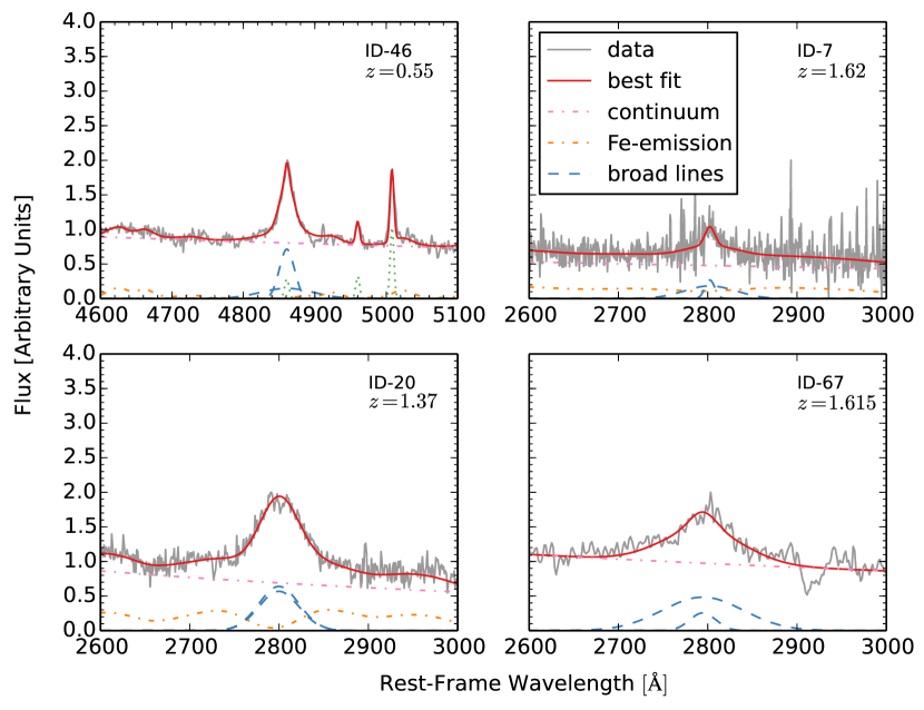
Figure 1.— Examples of multi-component fits to the broad H$\beta$ (the upper-left panel) or Mg ii emission lines. Dotted lines represent minor features (e.g., the [O iii] $\lambda\lambda 4959,5007$ lines and the narrow H$\beta$ component which are removed in the broad-line fit).

Figure 2.— Examples of two-component (AGN+galaxy) fits to SEDs (from the NUV to NIR). Red dotted (green dashed) lines represent the AGN (galaxy) component. Black solid lines show the summation of the galaxy and AGN SEDs. Note that each data point has a photometric error which is typically too small to be visible on this scale.

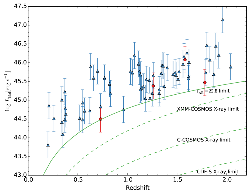
Figure 3.— The bolometric luminosity of AGNs (calculated by combining the X-ray observations and SED fitting) vs. redshift. Blue triangles represent AGNs that are detected in the observed-frame hard X-ray band ($2-10\ \rm{keV}$); red points are sources that are detected in the observed-frame soft X-ray band ($0.5-2\ \rm{keV}$) but not in the observed-frame hard X-ray band. The green solid line represent the limit introduced by $i_{\rm{AB}}=22.5$ which corresponds to the $\sim 90\%$ completeness of the optical spectroscopy for COSMOS sources (Trump et al., 2009a). The bolometric correction of the $i$ band is assumed to be $12$ (Richards et al., 2006) and the $K$ correction is made by assuming the optical-to-UV SED is a power-law with $\alpha_{\nu}=-0.44$ (Vanden Berk et al., 2001). The three green dashed lines represent the limits introduced by the X-ray sensitivity of the soft band of XMM-Newton/COSMOS and Chandra/COSMOS and the hard band of CDF-S, respectively. The bolometric correction of Hopkins et al. (2007) is assumed to calculate $L_{\rm Bol}$ from the X-ray sensitivity.

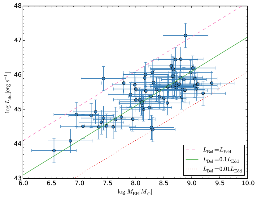
Figure 4.— The bolometric luminosity of AGNs vs. $M_{\rm BH}$. The pink dashed, green solid and red dotted lines correspond to the Eddington ratios of $1.0$, $0.1$ and $0.01$, respectively. For each object, the intrinsic scatter in the $L_{\rm Bol}$ and $M_{\rm BH}$ estimators ($0.35$ and $0.4$ dex, respectively) dominates the error. The Eddington ratios of our source spans from $0.01$ to $1.0$, typical range of BLAGNs (e.g., Kollmeier et al., 2006; Trump et al., 2009b, 2011; Lusso et al., 2012).

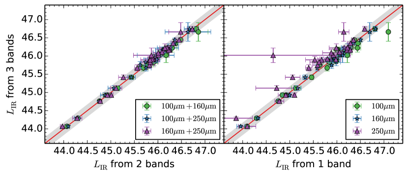
Figure 5.— Illustration of the reliability of estimating FIR luminosity using different Herschel bands. Left: Comparison of FIR luminosity estimated from two bands with that from all three bands. Right: Comparison of FIR luminosity estimated from one band with that from all three bands. The solid line and shaded area represent the ratio of unity and $0.17$ dex uncertainties. The two-band FIR estimator agrees well with the three-band estimator. Estimating SFR from a single band is also consistent with the three-band estimator. Note that there is a source in the right panel shows an extremely large uncertainty which is caused by the fact that the uncertainty of the flux in $250\ \rm{\mu m}$ for this source is large (if we take also the $100\ \rm{\mu m}$ and $160\ \rm{\mu m}$ bands into consideration, the uncertainty of this source is small).

Figure 6.— A comparison of SFR we measured with the expected SFR of star-forming main sequence galaxies with the same stellar mass. Our sources have a star formation activity which is marginally higher than that of the “main-sequence” (the mean of $\mathrm{SFR/SFR_{ms}}$ is $2$). This offset is due to an Eddington bias which is driven by the Herschel flux limit (see Section 4.1 for more details). The red dashed line represents the bias corrected $\mathrm{SFR/SFR_{ms}}$.

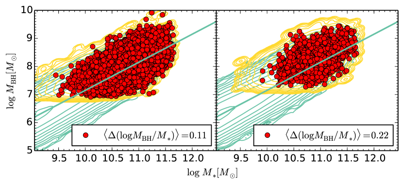
Figure 7.— Monte Carlo simulation of biases in our data. Left (right) panel is for $z=1.0$ ($z=2.0$). The green and yellow contours correspond to the PDFs of our mock sample and sample A (which results from the mock sample with a AGN luminosity cut off). For sample B, which results from sample A with a SFR cut off (i.e., sample B and our data share the same selection bias.), the actual distribution of simulated sources in the $M_{\rm{BH}}-M_{\ast}$ plane is plotted. The solid green lines correspond to $\log M_{\rm{BH}}=\log M_{\ast}-2.85$. See Section 4.1 for more details.

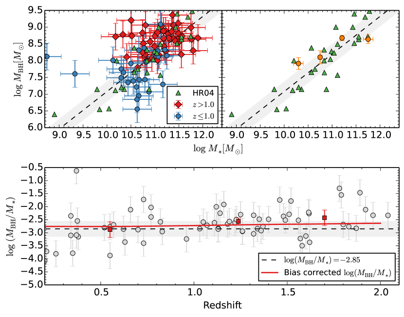
Figure 8.— Upper-left panel: The distribution of our BLAGNs in the $M_{\rm{BH}}-M_{\ast}$ plane. Upper-right panel: Sources are binned by $M_{\ast}$; four orange points represent the median values of $M_{\rm BH}$ and $M_{\ast}$ and their $1\sigma$ uncertainties (estimated via bootstrapping) for sources within four bins: $M_{\ast}<10^{10.5}\ M_{\odot}$, $10^{10.5}\ M_{\odot}\leq M_{\ast}<10^{11}\ M_{\odot}$, $10^{11}\ M_{\odot}\leq M_{\ast}<10^{11.5}\ M_{\odot}$, and $M_{\ast}\geq 10^{11.5}\ M_{\odot}$. The triangles in both panels represent sources from HR04. Lower panel: Logarithm of the ratio of the SMBH mass to the galaxy total stellar mass vs. redshift. Three red squares represent the mean value of the mass ratio and its $2\sigma$ uncertainty for sources with $z<1.0$, $1.0\leq z<1.5$, and $z\geq 1.5$. The red solid line represents the local HR04 relation as it would be observed under the biases of our sample. The lines and shaded regions in all panels represent the local SMBH mass-bulge mass relation by HR04 and its uncertainty. Our sources are indeed consistent with the biased HR04 relation, indicating no significant evolution of the $M_{\rm{BH}}-M_{\ast}$ relation.

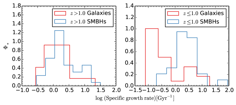
Figure 9.— Distributions of the specific SMBH and galaxy mass growth rates. The left (right) panel is for the high-(low-)redshift sub-sample. The specific galaxy growth rate distribution evolves significantly as a function of redshift while the specific SMBH growth rate distribution does not change dramatically. Note that $\Phi_{\ast}$ is the probability density function (i.e., $\int\Phi_{\ast}(x)\,\mathrm{d}x=1$).

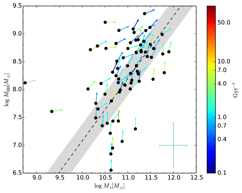
Figure 10.— The “flow patterns” of SMBHs and their host galaxies in the SMBH mass-galaxy total stellar mass plane. Arrows represent the direction of the evolution (45 degrees indicates $\log(\mathrm{s}\dot{M}/\mathrm{sSFR})=0$). Colors indicate the absolute value of the total specific growth rate (i.e., $\sqrt{\mathrm{s}\dot{M}^{2}+\mathrm{sSFR}^{2}}$) which spans $>2$ orders of magnitude. The dashed line and shaded area represent the local SMBH mass-bulge mass relation of HR04 and its uncertainty. The cross indicates the $1\sigma$ uncertainties of $M_{\rm{BH}}$ and $M_{\ast}$. The length of the vectors are arbitrary, since the “flow patterns” over a long timescale ($\simeq\ 1\ \mathrm{Gyr}$) depends on AGN duty cycle (see Section 6.3).

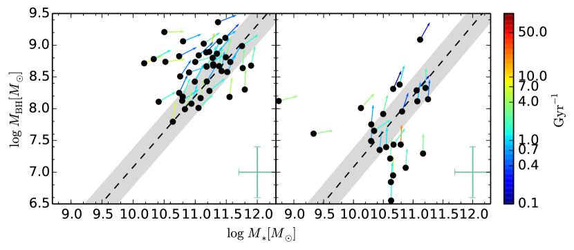
Figure 11.— The same as Figure 10, but for the high-redshift (left panel) and low-redshift (right panel) sub-samples.

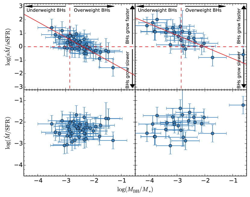
Figure 12.— Upper panels: The ratio of the SMBH to the host-galaxy specific mass growth rate vs. the ratio of the SMBH mass to the host-galaxy total stellar mass. Left (right) panels are for the high-(low-) redshift sub-samples. The red solid line in each panel represents the best fit. The best fit indicates an anti-correlation between $M_{\rm{BH}}/M_{\ast}$ and $\mathrm{s}\dot{M}/\mathrm{sSFR}$ is significant (null probability $p<10^{-6}$). The red vertical dashed line in each panel represents the local mass ratio from HR04. The red horizontal dashed line in each panel is an indicator of $\mathrm{s}\dot{M}/\mathrm{sSFR}=1$, i.e., the specific SMBH accretion rate and the specific SFR are equal. Note that there are more sources above the horizontal line. This asymmetric distribution indicates that, if the growth rates of our sources persist over some length of time, AGN duty cycle is less than unity (i.e., the lifetime of an active SMBH is smaller than the lifetime of star formation), otherwise the SMBH will become over-massive as we evolve our sources. Lower panels: The ratio of the SMBH accretion rate to SFR vs. the ratio of the SMBH mass to the host-galaxy total stellar mass. Again, left (right) panels are for the high-(low-) redshift sub-samples. A linear fit indicates that $\dot{M}/\mathrm{SFR}$ is a constant (with scatter) over $M_{\rm{BH}}/M_{\ast}$.

Figure 13.— The PDF of $\tau_{\rm{SF}}$ and $\rm AGN\ duty\ cycle$ (which measures the fraction of BLAGNs among star-forming galaxies, see Section 6.3) that would result in the largest fraction of our sources lying on the local SMBH mass-bulge mass relation. Left (right) panels are for the high-(low-) redshift sub-samples. The contour in each panel indicates the $1\sigma$ (i.e., $68.3\%$) uncertainty. The color map in each panel indicates the probability density.

Table 1Summary of Sample Selection

Selection Criteria	COSMOS	CDF-S
Total $z<2.4$ X-ray BLAGNs	221	30
X-ray BLAGNs with optical/UV and Herschel photometry	85	11
Final sample: X-ray BLAGNs with optical/UV photometry, robust IR luminosity, good spectra	62	7

Table 2Summary of Properties of AGNs and Host Galaxies

ID	RA	DEC	$z$	SF	Field	$\log M_{\rm{BH}}$	$\log M_{\ast}$	$\log L_{\rm{Bol}}$	$\log L_{\rm{IR}}$	$\Delta(\log L_{\rm{IR}})$
	deg	deg				$M_{\odot}$	$M_{\odot}$	$\rm{erg\ s^{-1}}$	$\rm{erg\ s^{-1}}$	$\rm{erg\ s^{-1}}$
1	149.83875	2.67511	0.26	S	COSMOS	7.07	10.88	44.51	44.93	0.06
2	150.15837	2.13961	1.83	Z	COSMOS	8.99	11.75	46.08	46.74	0.07
3	150.34592	2.14758	1.26	Z	COSMOS	8.28	11.23	45.38	46.17	0.08
4	150.0425	2.62917	1.57	Z	COSMOS	8.68	11.90	46.16	46.44	0.05
5	149.69879	2.44122	1.52	I	COSMOS	8.74	10.52	45.77	46.17	0.07
6	149.881	2.45083	1.32	Z	COSMOS	8.01	11.05	45.28	46.11	0.02
7	149.99158	1.72428	1.62	S	COSMOS	8.19	11.55	46.02	46.23	0.04
8	150.30954	2.39914	1.80	S	COSMOS	8.81	11.49	46.46	46.35	0.04
9	150.62525	1.80289	0.63	I	COSMOS	7.43	10.79	45.90	45.67	0.09
10	150.05871	2.47739	1.26	Z	COSMOS	8.58	11.52	45.66	46.03	0.03
11	149.70587	2.41975	1.12	Z	COSMOS	9.36	11.37	45.77	45.92	0.03
12	149.94171	2.79544	1.07	S	COSMOS	8.67	11.38	46.19	45.90	0.07
13	149.58283	2.48433	0.34	S	COSMOS	8.15	11.25	45.01	44.76	0.01
14	150.12508	2.86175	1.58	I	COSMOS	8.30	11.80	46.08	45.90	0.06
15	150.32737	2.46094	1.05	I	COSMOS	8.70	11.29	45.73	45.75	0.10
16	149.59246	1.75675	1.96	S	COSMOS	8.90	11.23	47.15	46.66	0.26
17	150.14708	2.71747	1.18	Z	COSMOS	8.13	10.79	45.05	45.63	0.12
18	150.19558	2.00442	1.92	Z	COSMOS	9.02	11.14	46.20	46.22	0.11
19	150.63387	2.59369	0.66	S	COSMOS	8.01	10.12	45.59	45.42	0.06
20	150.49567	2.41256	1.37	Z	COSMOS	8.43	11.19	45.37	45.64	0.16
21	150.57633	2.18142	0.55	I	COSMOS	8.29	11.06	44.48	44.93	0.00
22	150.64521	2.71481	0.20	S	COSMOS	6.55	10.63	43.81	44.07	0.04
23	150.19504	1.79383	1.87	I	COSMOS	8.74	11.57	45.69	46.09	0.10
24	149.41992	2.03553	1.48	I	COSMOS	9.12	11.49	45.74	45.84	0.10
25	150.58187	2.28769	1.34	Z	COSMOS	7.99	10.83	45.72	45.90	0.09
26	149.47792	2.64247	1.6	S	COSMOS	8.64	11.77	46.26	45.94	0.22
27	149.86558	2.00306	1.25	Z	COSMOS	8.11	10.41	45.19	45.47	0.10
28	149.64183	2.74089	1.89	S	COSMOS	8.72	10.18	46.45	46.03	0.24
29	150.658	2.7835	0.21	I	COSMOS	6.95	10.66	44.85	44.29	0.04
30	150.55487	2.641	1.14	Z	COSMOS	8.51	10.76	45.33	45.14	0.35
31	149.58521	2.05111	1.35	Z	COSMOS	8.80	11.28	45.93	45.77	0.29
32	150.19975	2.19089	1.51	Z	COSMOS	8.89	11.18	45.56	45.57	0.16
33	150.11929	2.85353	0.77	I	COSMOS	9.09	11.12	45.60	45.12	0.07
34	150.31367	2.80361	1.46	I	COSMOS	9.06	10.80	45.69	45.58	0.25
35	149.91692	2.38522	1.13	I	COSMOS	8.59	11.42	45.68	45.41	0.22
36	149.78971	2.32125	0.38	I	COSMOS	7.39	10.55	44.63	44.14	0.01
37	150.6355	1.66917	1.79	I	COSMOS	8.78	10.33	45.74	45.31	0.62
38	150.30004	2.70936	0.73	I	COSMOS	7.61	9.33	44.50	44.77	0.09
39	150.13954	1.6365	0.52	Z	COSMOS	7.49	10.30	44.53	43.93	1.41
40	150.23083	2.57817	1.40	Z	COSMOS	8.87	11.35	45.87	46.02	0.20
41	150.80187	2.00061	1.78	I	COSMOS	9.21	10.50	45.47	46.06	0.07
42	150.62771	2.741	0.82	I	COSMOS	7.92	10.50	45.43	45.12	0.10
43	150.384	1.57247	1.36	S	COSMOS	8.17	11.09	45.92	45.85	0.11
44	150.25267	2.48642	2.04	I	COSMOS	9.06	11.39	45.89	46.16	0.13
45	150.24517	1.90008	1.56	S	COSMOS	8.66	11.18	45.97	45.97	0.04
46	150.19467	2.06792	0.55	I	COSMOS	7.29	11.17	44.93	44.77	0.08
47	150.13908	1.877	0.83	I	COSMOS	8.12	11.07	45.18	45.09	0.01
48	150.006	2.81242	0.77	S	COSMOS	8.38	10.77	45.59	45.10	0.10
49	149.86796	2.35192	0.35	I	COSMOS	6.84	10.63	44.09	44.51	0.02
50	149.62429	2.18067	1.19	I	COSMOS	8.43	10.99	45.55	45.57	0.13
51	149.4795	2.80183	1.11	S	COSMOS	8.68	11.29	45.97	45.37	0.19
52	149.868	2.33075	1.49	I	COSMOS	8.67	11.18	45.67	46.10	0.07
53	150.55046	1.709	0.37	I	COSMOS	7.35	10.44	44.49	44.34	0.08
54	149.6692	2.07406	0.34	Z	COSMOS	8.31	10.67	44.42	44.17	0.10
55	150.10521	1.98117	0.37	S	COSMOS	8.12	8.75	45.23	44.18	0.13
56	150.05379	2.58967	0.7	S	COSMOS	8.33	11.21	45.78	44.88	0.11
57	150.1237	2.35825	0.73	Z	COSMOS	7.21	10.62	44.83	44.91	0.11
58	150.68317	2.57461	0.38	Z	COSMOS	7.75	10.31	44.78	44.07	0.12
59	150.2082	1.87536	1.16	I	COSMOS	8.83	10.74	45.36	45.31	0.14
60	149.89484	2.17444	1.32	Z	COSMOS	8.57	10.90	45.19	45.75	0.09
61	149.76346	2.33411	1.13	Z	COSMOS	8.08	10.94	45.28	45.37	0.13
62	149.66362	2.08519	1.22	Z	COSMOS	8.19	10.80	45.54	45.48	0.13
63	53.22033	-27.85556	1.23	S04	CDF-S	8.25	10.74	45.06	44.96	0.07
64	53.11037	-27.67658	1.03	S04	CDF-S	7.80	10.64	45.77	45.55	0.02
65	53.10483	-27.70525	1.62	S04	CDF-S	8.74	11.00	45.64	46.15	0.04
66	53.07146	-27.71761	0.57	S04	CDF-S	7.65	10.35	44.72	45.33	0.14
67	53.0455	-27.73756	1.615	S04	CDF-S	8.84	11.06	45.58	45.58	0.01
68	53.25642	-27.76183	0.62	S04	CDF-S	7.96	10.82	44.72	44.85	0.03
69	53.12525	-27.75656	0.96	S04	CDF-S	7.43	10.67	44.75	45.59	0.02

Note. —

References

- Alexander & Hickox (2012) Alexander, D. M., & Hickox, R. C. 2012, New Astron. Rev., 56, 93
- Arnouts et al. (2007) Arnouts, S., Walcher, C. J., Le Fèvre, O., et al. 2007, A&A, 476, 137
- Astropy Collaboration et al. (2013) Astropy Collaboration, Robitaille, T. P., Tollerud, E. J., et al. 2013, A&A, 558, A33
- Babić et al. (2007) Babić, A., Miller, L., Jarvis, M. J., et al. 2007, A&A, 474, 755
- Bennert et al. (2011) Bennert, V. N., Auger, M. W., Treu, T., Woo, J.-H., & Malkan, M. A. 2011, ApJ, 742, 107
- Bentz et al. (2006) Bentz, M. C., Peterson, B. M., Pogge, R. W., Vestergaard, M., & Onken, C. A. 2006, ApJ, 644, 133
- Bongiorno et al. (2012) Bongiorno, A., Merloni, A., Brusa, M., et al. 2012, MNRAS, 427, 3103
- Bournaud et al. (2012) Bournaud, F., Juneau, S., Le Floc’h, E., et al. 2012, ApJ, 757, 81
- Bourne et al. (2014) Bourne, M. A., Nayakshin, S., & Hobbs, A. 2014, arXiv:1405.5647
- Brammer et al. (2012) Brammer, G. B., van Dokkum, P. G., Franx, M., et al. 2012, ApJS, 200, 13
- Brandt & Alexander (2010) Brandt, W. N., & Alexander, D. M. 2010, Proceedings of the National Academy of Science, 107, 7184
- Brusa et al. (2010) Brusa, M., Civano, F., Comastri, A., et al. 2010, ApJ, 716, 348
- Bruzual & Charlot (2003) Bruzual, G., & Charlot, S. 2003, MNRAS, 344, 1000
- Calzetti et al. (2000) Calzetti, D., Armus, L., Bohlin, R. C., et al. 2000, ApJ, 533, 682
- Capak et al. (2007) Capak, P., Aussel, H., Ajiki, M., et al. 2007, ApJS, 172, 99
- Cappelluti et al. (2009) Cappelluti, N., Brusa, M., Hasinger, G., et al. 2009, A&A, 497, 635
- Cardamone et al. (2010) Cardamone, C. N., van Dokkum, P. G., Urry, C. M., et al. 2010, ApJS, 189, 270
- Chabrier (2003) Chabrier, G. 2003, PASP, 115, 763
- Chary & Elbaz (2001) Chary, R., & Elbaz, D. 2001, ApJ, 556, 562
- Chen et al. (2013) Chen, C.-T. J., Hickox, R. C., Alberts, S., et al. 2013, ApJ, 773, 3
- Cisternas et al. (2011) Cisternas, M., Jahnke, K., Inskip, K. J., et al. 2011, ApJ, 726, 57
- Civano et al. (2013) Civano, F. M., et al. 2013, AAS/High Energy Astrophysics Division, 13, #116.18
- Civano et al. (2012) Civano, F., Elvis, M., Brusa, M., et al. 2012, ApJS, 201, 30
- Collin et al. (2006) Collin, S., Kawaguchi, T., Peterson, B. M., & Vestergaard, M. 2006, A&A, 456, 75
- Cook & Stefanski (1994) Cook, J. R., & Stefanski, L. A. 1994, JASA, 89, 428
- Dale & Helou (2002) Dale, D. A., & Helou, G. 2002, ApJ, 576, 159
- Davis & Laor (2011) Davis, S. W., & Laor, A. 2011, ApJ, 728, 98
- Dekel et al. (2009) Dekel, A., Sari, R., & Ceverino, D. 2009, ApJ, 703, 785
- Di Matteo et al. (2005) Di Matteo, T., Springel, V., & Hernquist, L. 2005, Nature, 433, 604
- Elbaz et al. (2007) Elbaz, D., Daddi, E., Le Borgne, D., et al. 2007, A&A, 468, 33
- Elbaz et al. (2011) Elbaz, D., Dickinson, M., Hwang, H. S., et al. 2011, A&A, 533, A119
- Elvis et al. (2009) Elvis, M., Civano, F., Vignali, C., et al. 2009, ApJS, 184, 158
- Fabian (2012) Fabian, A. C. 2012, ARA&A, 50, 455
- Ferrarese & Merritt (2000) Ferrarese, L., & Merritt, D. 2000, ApJ, 539, L9
- Fontana et al. (2006) Fontana, A., Salimbeni, S., Grazian, A., et al. 2006, A&A, 459, 745
- Gabor & Bournaud (2014) Gabor, J. M., & Bournaud, F. 2014, MNRAS, 441, 1615
- Gabor et al. (2009) Gabor, J. M., Impey, C. D., Jahnke, K., et al. 2009, ApJ, 691, 705
- Gebhardt et al. (2000) Gebhardt, K., Bender, R., Bower, G., et al. 2000, ApJ, 539, L13
- Georgakakis et al. (2009) Georgakakis, A., Coil, A. L., Laird, E. S., et al. 2009, MNRAS, 397, 623
- Gültekin et al. (2009) Gültekin, K., Richstone, D. O., Gebhardt, K., et al. 2009, ApJ, 698, 198
- Häring & Rix (2004) Häring, N., & Rix, H.-W. 2004, ApJ, 604, L89
- Hickox et al. (2014) Hickox, R. C., Mullaney, J. R., Alexander, D. M., et al. 2014, ApJ, 782, 9
- Ho (2008) Ho, L. C. 2008, ARA&A, 46, 475
- Hopkins et al. (2006) Hopkins, P. F., Somerville, R. S., Hernquist, L., et al. 2006, ApJ, 652, 864
- Hopkins et al. (2007) Hopkins, P. F., Richards, G. T., & Hernquist, L. 2007, ApJ, 654, 731
- Hopkins et al. (2009) Hopkins, P. F., Hickox, R., Quataert, E., & Hernquist, L. 2009, MNRAS, 398, 333
- Hopkins et al. (2010) Hopkins, P. F., Bundy, K., Croton, D., et al. 2010, ApJ, 715, 202
- Ilbert et al. (2009) Ilbert, O., Capak, P., Salvato, M., et al. 2009, ApJ, 690, 1236
- Ilbert et al. (2010) Ilbert, O., Salvato, M., Le Floc’h, E., et al. 2010, ApJ, 709, 644
- Jahnke et al. (2009) Jahnke, K., Bongiorno, A., Brusa, M., et al. 2009, ApJ, 706, L215
- Jahnke & Macciò (2011) Jahnke, K., & Macciò, A. V. 2011, ApJ, 734, 92
- Kaspi et al. (2007) Kaspi, S., Brandt, W. N., Maoz, D., et al. 2007, ApJ, 659, 997
- Kelly & Shen (2013) Kelly, B. C., & Shen, Y. 2013, ApJ, 764, 45
- Kennicutt (1998) Kennicutt, R. C., Jr. 1998, ARA&A, 36, 189
- King (2003) King, A. 2003, ApJ, 596, L27
- Kirkpatrick et al. (2012) Kirkpatrick, A., Pope, A., Alexander, D. M., et al. 2012, ApJ, 759, 139
- Kocevski et al. (2012) Kocevski, D. D., Faber, S. M., Mozena, M., et al. 2012, ApJ, 744, 148
- Kollmeier et al. (2006) Kollmeier, J. A., Onken, C. A., Kochanek, C. S., et al. 2006, ApJ, 648, 128
- Kormendy & Ho (2013) Kormendy, J., & Ho, L. C. 2013, ARA&A, 51, 511
- Lang et al. (2014) Lang, P., Wuyts, S., Somerville, R. S., et al. 2014, ApJ, 788, 11
- Lauer et al. (2007) Lauer, T. R., Tremaine, S., Richstone, D., & Faber, S. M. 2007, ApJ, 670, 249
- Lilly et al. (2007) Lilly, S. J., Le Fèvre, O., Renzini, A., et al. 2007, ApJS, 172, 70
- Luo et al. (2008) Luo, B., Bauer, F. E., Brandt, W. N., et al. 2008, ApJS, 179, 19
- Luo et al. (2010) Luo, B., Brandt, W. N., Xue, Y. Q., et al. 2010, ApJS, 187, 560
- Lusso et al. (2012) Lusso, E., Comastri, A., Simmons, B. D., et al. 2012, MNRAS, 425, 623
- Lutz et al. (2011) Lutz, D., Poglitsch, A., Altieri, B., et al. 2011, A&A, 532, A90
- Magnelli et al. (2013) Magnelli, B., Popesso, P., Berta, S., et al. 2013, A&A, 553, A132
- Magorrian et al. (1998) Magorrian, J., Tremaine, S., Richstone, D., et al. 1998, AJ, 115, 2285
- Marconi & Hunt (2003) Marconi, A., & Hunt, L. K. 2003, ApJ, 589, L21
- Maronna et al. (2006) Maronna, R. A., Martin, R. D., & Yohai, V. J. 2006, Robust Statistics: Theory and Methods (1st ed.; Chichester: Wiley)
- Matsuoka et al. (2013) Matsuoka, K., Silverman, J. D., Schramm, M., et al. 2013, ApJ, 771, 64
- Matsuoka et al. (2014) Matsuoka, Y., Strauss, M. A., Price, T. N., III, & DiDonato, M. S. 2014, ApJ, 780, 162
- McCracken et al. (2010) McCracken, H. J., Capak, P., Salvato, M., et al. 2010, ApJ, 708, 202
- Merloni et al. (2010) Merloni, A., Bongiorno, A., Bolzonella, M., et al. 2010, ApJ, 708, 137
- Mullaney et al. (2012) Mullaney, J. R., Daddi, E., Béthermin, M., et al. 2012, ApJ, 753, L30
- Muzzin et al. (2013) Muzzin, A., Marchesini, D., Stefanon, M., et al. 2013, ApJ, 777, 18
- Narayan & Yi (1995) Narayan, R., & Yi, I. 1995, ApJ, 452, 710
- Noeske et al. (2007) Noeske, K. G., Weiner, B. J., Faber, S. M., et al. 2007, ApJ, 660, L43
- Nordon et al. (2012) Nordon, R., Lutz, D., Genzel, R., et al. 2012, ApJ, 745, 182
- Oliver et al. (2012) Oliver, S. J., Bock, J., Altieri, B., et al. 2012, MNRAS, 424, 1614
- Onken et al. (2004) Onken, C. A., Ferrarese, L., Merritt, D., et al. 2004, ApJ, 615, 645
- Onken et al. (2007) Onken, C. A., Valluri, M., Peterson, B. M., et al. 2007, ApJ, 670, 105
- Peng et al. (2006) Peng, C. Y., Impey, C. D., Rix, H.-W., et al. 2006, ApJ, 649, 616
- Peng (2007) Peng, C. Y. 2007, ApJ, 671, 1098
- Peterson (1997) Peterson, B. M. 1997, An introduction to active galactic nuclei, Publisher: Cambridge, New York Cambridge University Press, 1997 Physical description xvi, 238 p. ISBN 0521473489,
- Pozzetti et al. (2007) Pozzetti, L., Bolzonella, M., Lamareille, F., et al. 2007, A&A, 474, 443
- Prevot et al. (1984) Prevot, M. L., Lequeux, J., Prevot, L., Maurice, E., & Rocca-Volmerange, B. 1984, A&A, 132, 389
- Rafferty et al. (2011) Rafferty, D. A., Brandt, W. N., Alexander, D. M., et al. 2011, ApJ, 742, 3
- Richards et al. (2006) Richards, G. T., Lacy, M., Storrie-Lombardi, L. J., et al. 2006, ApJS, 166, 470
- Roos et al. (2014) Roos, O., Juneau, S., Bournaud, F., & Gabor, J. M. 2014, arXiv:1405.7971
- Rosario et al. (2012) Rosario, D. J., Santini, P., Lutz, D., et al. 2012, A&A, 545, A45
- Rosario et al. (2013a) Rosario, D. J., Santini, P., Lutz, D., et al. 2013a, ApJ, 771, 63
- Rosario et al. (2013b) Rosario, D. J., Trakhtenbrot, B., Lutz, D., et al. 2013b, A&A, 560, A72
- Sanders et al. (2007) Sanders, D. B., Salvato, M., Aussel, H., et al. 2007, ApJS, 172, 86
- Schawinski et al. (2011) Schawinski, K., Treister, E., Urry, C. M., et al. 2011, ApJ, 727, L31
- Schlegel et al. (1998) Schlegel, D. J., Finkbeiner, D. P., & Davis, M. 1998, ApJ, 500, 525
- Schramm & Silverman (2013) Schramm, M., & Silverman, J. D. 2013, ApJ, 767, 13
- Schulze & Wisotzki (2014) Schulze, A., & Wisotzki, L. 2014, MNRAS, 438, 3422
- Scoville et al. (2007) Scoville, N., Aussel, H., Brusa, M., et al. 2007, ApJS, 172, 1
- Shen et al. (2008) Shen, Y., Greene, J. E., Strauss, M. A., Richards, G. T., & Schneider, D. P. 2008, ApJ, 680, 169
- Shen & Kelly (2010) Shen, Y., & Kelly, B. C. 2010, ApJ, 713, 41
- Shen & Liu (2012) Shen, Y., & Liu, X. 2012, ApJ, 753, 125
- Shen et al. (2014) Shen, Y., Brandt, W. N., Dawson, K. S., et al. 2014, arXiv:1408.5970
- Silk & Rees (1998) Silk, J., & Rees, M. J. 1998, A&A, 331, L1
- Silverman et al. (2009) Silverman, J. D., Lamareille, F., Maier, C., et al. 2009, ApJ, 696, 396
- Skelton et al. (2014) Skelton, R. E., Whitaker, K. E., Momcheva, I. G., et al. 2014, arXiv:1403.3689
- Soltan (1982) Soltan, A. 1982, MNRAS, 200, 115
- Szokoly et al. (2004) Szokoly, G. P., Bergeron, J., Hasinger, G., et al. 2004, ApJS, 155, 271
- Tremaine et al. (2002) Tremaine, S., Gebhardt, K., Bender, R., et al. 2002, ApJ, 574, 740
- Treu et al. (2007) Treu, T., Woo, J.-H., Malkan, M. A., & Blandford, R. D. 2007, ApJ, 667, 117
- Trump et al. (2009a) Trump, J. R., Impey, C. D., Elvis, M., et al. 2009a, ApJ, 696, 1195
- Trump et al. (2009b) Trump, J. R., Impey, C. D., Kelly, B. C., et al. 2009b, ApJ, 700, 49
- Trump et al. (2011) Trump, J. R., Impey, C. D., Kelly, B. C., et al. 2011, ApJ, 733, 60
- Trump et al. (2013) Trump, J. R., Hsu, A. D., Fang, J. J., et al. 2013, ApJ, 763, 133
- Trump et al. (2014) Trump, J. R., Barro, G., Juneau, S., et al. 2014, arXiv:1407.7525
- Vanden Berk et al. (2001) Vanden Berk, D. E., Richards, G. T., Bauer, A., et al. 2001, AJ, 122, 549
- Vestergaard & Osmer (2009) Vestergaard, M., & Osmer, P. S. 2009, ApJ, 699, 800
- Vestergaard & Peterson (2006) Vestergaard, M., & Peterson, B. M. 2006, ApJ, 641, 689
- Vestergaard & Wilkes (2001) Vestergaard, M., & Wilkes, B. J. 2001, ApJS, 134, 1
- Vito et al. (2014) Vito, F., Maiolino, R., Santini, P., et al. 2014, arXiv:1403.7966
- Wang et al. (2013) Wang, L., Viero, M., Clarke, C., et al. 2013, arXiv:1312.0552
- Whitaker et al. (2012) Whitaker, K. E., van Dokkum, P. G., Brammer, G., & Franx, M. 2012, ApJ, 754, L29
- Xue et al. (2010) Xue, Y. Q., Brandt, W. N., Luo, B., et al. 2010, ApJ, 720, 368
- Xue et al. (2011) Xue, Y. Q., Luo, B., Brandt, W. N., et al. 2011, ApJS, 195, 10
- York et al. (2000) York, D. G., Adelman, J., Anderson, J. E., Jr., et al. 2000, AJ, 120, 1579
- Yuan & Narayan (2014) Yuan, F., & Narayan, R. 2014, ARA&A, 52, 529