A Pólya Urn Document Language Model for Improved Information Retrieval

Abstract

The multinomial language model has been one of the most effective models of retrieval for over a decade. However, the multinomial distribution does not model one important linguistic phenomenon relating to term-dependency, that is the tendency of a term to repeat itself within a document (i.e. word burstiness). In this article, we model document generation as a random process with reinforcement (a multivariate Pólya process) and develop a Dirichlet compound multinomial language model that captures word burstiness directly.

We show that the new reinforced language model can be computed as efficiently as current retrieval models, and with experiments on an extensive set of TREC collections, we show that it significantly outperforms the state-of-the-art language model for a number of standard effectiveness metrics. Experiments also show that the tuning parameter in the proposed model is more robust than in the multinomial language model. Furthermore, we develop a constraint for the verbosity hypothesis and show that the proposed model adheres to the constraint. Finally, we show that the new language model essentially introduces a measure closely related to idf which gives theoretical justification for combining the term and document event spaces in tf-idf type schemes.

Ronan Cummins, Jiaul H. Paik, and Yuanhua Lv, 2015. A Pólya Urn Document Language Model for Improved Information Retrieval.

Author’s addresses: Ronan Cummins, The Computer Laboratory, University of Cambridge; Jiaul H. Paik, College of Computer, Mathematical, and Natural Sciences, University of Maryland; Yuanhua Lv, Microsoft Research;

1 Introduction

Language modelling approaches to information retrieval have become increasingly popular since the original works ponte98; hiemstra98; hiemstra00; lavrenko01; zhai01. They afford a particularly appealing view of the retrieval problem due in part to the principled nature in which a retrieval function can be mathematically derived. The query likelihood method ponte98 is one of the most widely-adopted approaches to retrieval, and ranks documents based on the likelihood of their document language model generating the query string. The most widely-accepted multinomial language model treats the document model as a multinomial distribution over the terms, where the parameters of each document model are estimated using the observations from the actual document smoothed with the entire collection using the Dirichlet prior smoothing method zhai01.

One main deficiency with using a multinomial distribution as a language model is that all term occurrences are treated independently. The term-independence assumption in information retrieval is often adopted in theory and practice as it renders the retrieval problem tractable, simplifies the implementation of many models, and has been shown to be suitably effective. Although retrieval approaches that incorporate term-dependencies metzler05; zhao09; lv09:02; cummins09; bendersky12 have been shown in general to be more effective, they are computationally more complex. Therefore, a language modelling approach that has the same complexity as a unigram language model but also incorporates dependencies, would be a useful contribution as it would likely exhibit increased effectiveness at no extra computational cost. In fact, the use of the multinomial distribution in the standard language modelling approach ignores two types of dependencies; namely, the dependency between distinct terms (word types) and the dependency between recurrences of the same term (word tokens). It is this second type of dependency that we address in this article.

It is well known that once a term occurs in a document, it is more likely to re-appear in the same document. This phenomenon is known as word burstiness church95; madsen05, and is a type of dependency that is not modelled in the multinomial language model zhai04. Essentially, word burstiness can be defined as the tendency of an otherwise rare term to occur multiple times in a document, and can be seen as a form of preferential attachment simon55; mitzenmacher03. One theory for this phenomenon is that an author tends to sample terms previously written in the same document to form association simon55. The process of association of similar concepts throughout a document using the same lexical form may aid coherence, readability, and understanding. For example, if an author starts to use the term pavement in an article, he/she intuitively tends to continue its usage throughout the document, rather than changing to one of its synonyms (e.g. sidewalk or footpath).

On the other hand, queries are requests for information and are generated with a different motive in mind. When requesting or searching for information a user is more likely to expand the vocabulary used in the query (and possibly make use of synonyms) in the hope of matching those query-terms contained in relevant documents. Furthermore, queries are usually much shorter than documents and as a result, we assume that queries are less likely to exhibit word-burstiness. That is not to say that a certain term could not appear multiple times in a query, it simply suggests that the reason for it reappearing is different than in a document. For these reasons we model documents and queries using different generative assumptions.

This article presents the SPUD (Smoothed Pólya Urn Document) language model that incorporates word burstiness only into the document model. We use the Dirichlet compound multinomial (DCM), also known as the multivariate Pólya distribution, to model documents in place of the standard multinomial distribution, while we use the standard multinomial to model query generation. We show that this new retrieval model obtains significantly increased effectiveness compared to the current state-of-the-art model on a range of datasets for a number of effectiveness metrics. This article is organized as follows. Section 2 introduces notation used in the remainder of the article and also presents a comprehensive review of relevant research. Section 3 reviews the standard language modelling approach. Section 4 presents the SPUD language model. Section 5 outlines efficient forms of the new retrieval functions, and provides deep insights into the proposed functions. The experimental design and results are presented in Section 6. Section 7 presents a discussion of the results and Section 8 concludes with a summary.

2 Related Research

In this section we review related work in language models and word burstiness, before outlining the main contributions of this work. Table 2 introduces notation used in the remainder of this article.

Feature Notation

Key	Description
$c(t,d)$	frequency of term $t$ in document $d$
$c(t,q)$	frequency of term $t$ in query $q$
$|d|$	length of document $d$ (i.e. number of word tokens)
$\vec{|d|}$	length of document vector (# of distinct terms in document $d$ )
$cf_{t}$	collection frequency (frequency of $t$ in the entire collection )
$df_{t}$	document frequency (number of documents in which $t$ occurs)
$|q|$	length of query $q$ (i.e. number of word tokens)
$|c|$	number of tokens in the entire collection $c$
$n$	number of documents in the collection
$|{v}|$	vocabulary of the collection (# of distinct terms in the collection)

2.1 Query Likelihood

The predominant method of ranking documents using the language modelling approach remains the query likelihood method of ponte98. In the query likelihood method, documents are ranked based on the likelihood of their document model, $\mathcal{M}_{d}$, generating the query string. The following equation shows how the query likelihood, $p(q|\mathcal{M}_{d})$, is calculated for a unigram multinomial language model:

$$p(q|\mathcal{M}_{d}=\bm{\theta}_{dm})=\prod_{t\in q}p(t|\bm{\theta}_{dm})^{c(t,q)}$$ (1)

where $q$ is the query string and $\bm{\theta}_{dm}$ is the multinomial document language model. The effectiveness of this retrieval method crucially depends on the estimation of the document model $\bm{\theta}_{dm}$. It is typically estimated using the actual document $d$ and is smoothed with the background language model which is estimated from the entire collection $c$. When using a multinomial, the query likelihood method (Eq. 1) can be rewritten in a rank equivalent form as follows:

$$log\;p(q|\mathcal{M}_{d}=\bm{\theta}_{dm})=\sum_{t\in q}(log\;p(t|\bm{\theta}_{dm})\cdot{c(t,q)})$$ (2)

which shows that, as with most other retrieval functions (e.g. BM25 robertson96), the scoring function comprises a summation of query-term weights. If $p(t|\bm{\theta}_{dm})$ is estimated using only the maximum-likelihood estimates of a term occurring in a document (i.e. $c(t,d)/|d|$), over-fitting would occur. For instance, this would result in any document that did not contain all query-terms not being retrieved, as its document model deemed to have generated the query with a probability of zero (see Eq. 1). It should also be noted that when substituting the maximum likelihood probabilities ($c(t,d)/|d|$) into Eq. (2), the weight of each term becomes $log(c(t,d)/|d|)$ which has the effect of reducing the weight contribution of successive occurrences of the same term to a document score. This non-linear term-frequency effect has been often reported as a useful heuristic in IR fang04; fang05; cummins07; clinchant10; clinchantg11; lv12. However, in the multinomial query likelihood retrieval method this non-linearity is only the consequence of a mathematical transformation, and the actual dependency between successive occurrences of the same term is not modelled.

2.2 Advances in Language Models

Since the initial work applying language models ponte98; hiemstra98 to information retrieval, there have been a number of advances in terms of both theory and practice. Graph-based models gao04; metzler05; blanco12; bendersky12 that capture aspects of term-dependency have been shown to improve retrieval performance over unigram models. Furthermore, positional-based language models zhao09; lv10 have been proposed and incorporate term dependencies that often span several terms. In general, the incorporation of term-dependency information in larger web collections has been shown to be beneficial to retrieval quality.

Although many language modelling approaches to information retrieval use the query-likelihood approach to ranking, it is not the only means of inducing a ranking using language models. In particular, relevance-based language models lavrenko01 estimate a relevance model from which all relevant documents for a particular information need are assumed to have been drawn. The approach to ranking in that work is similar to the classic probabilistic document retrieval approaches jones00, where documents are ranked based on the odds of being drawn from the relevant class compared to non-relevant class. The relevance-based language modelling approach provides a principled mechanism in which the retrieval model can be updated as relevant and non-relevant documents become known. This approach led to the development of pseudo-relevance query expansion language models umass4; diaz06; lv10.

The language modelling approach has now become a starting point from which more complex models can be built. Aside from pseudo-relevance query expansion, other approaches such as latent Dirichlet allocation (LDA) have been incorporated into ad-hoc retrieval wei06. In essence, improving the retrieval effectiveness of the standard language modelling approach to information retrieval can ultimately benefit any of the myriad of approaches which depend upon it (e.g. pseudo-relevance feedback).

2.3 Word Burstiness

The modelling of word burstiness in documents has been addressed before in text-related tasks, but it has not been incorporated with the query likelihood method in information retrieval. madsen05 use the DCM distribution to model word burstiness and demonstrate its effectiveness on document classification. They estimate a DCM model for each class from training data. They then classify an unseen document to a specific class according to the mostly likely generative DCM class model. They show that this DCM model outperforms the more standard multinomial model. The information retrieval task is somewhat different as it deals with both documents and queries. In our work we have different generative assumptions for both documents and queries. A further difference is that in the classification task there are a number of documents from which we can infer a particular class model, while in the query-likelihood approach to information retrieval we have access to only one instance of a document from the document model.

Due to the complexity of estimating parameters for the DCM, elkan06 developed an approximate distribution (the EDCM) and demonstrated its effectiveness for clustering. We make use of this approximation later in this article. The DCM has also been used in a hypergeometric language model tsagkias11 for modelling the characteristics of very long queries. In other work, a two-stage language modelling approach has been developed goldwater11 that generates words according to the power-law characteristics of natural language. They decompose the language generation process into a generator, which creates instances of word types, and an adaptor which has the tendency to repeat those specific word types. Further arguments which link preferential attachment to the power-law characteristics of natural language are reviewed by mitzenmacher03. cowans04 uses a hierarchical Dirichlet process to arrive at a ranking function which is reported as being superior to BM25. Related work sunehag07 provides some interesting connections between the traditional tf-idf weighting scheme and the two-stage generator-adaptor models. Our work is more extensive and actually develops a document language model from which retrieval functions are derived.

In recent work, an extension of earlier information-based approaches amati02 is developed that incorporates burstiness in a log-logistic retrieval function clinchantg09; clinchantg11. The authors develop a means for identifying if a term-frequency distribution is bursty. They conclude that the frequency distribution must be a type of power-law (or Pareto-type) distribution. Our work is much more in the spirit of generative language modelling where the term-frequency aspect occurs naturally from the model (in our case a hierarchical Bayesian approach) to introduce dependencies between subsequent occurrences of the same term. Our model also exhibits power-law characteristics consistent with the work by clinchantg11.

The work most similar to ours uses the DCM distribution to develop a probabilistic relevance-based language model xu08; xu10. For each query they estimate a relevant and non-relevant DCM model and it is assumed that all documents are generated from either of those two models. However, our work does not assume a relevance model and instead, assumes that each document is generated from a different document model. This means that we model burstiness on a per document basis, rather than modelling burstiness for a set of relevant (and non-relevant) documents. It is more likely that different documents are bursty to different degrees as they were written by different authors, and this is not modelled in the relevance-based approach of Xu and Akella. Our model is a query-likelihood approach using different generative assumptions for both the document and query, and leads to retrieval functions that are distinct from those in the aforementioned relevance-based approach.

Although xu08 report some improvement in retrieval effectiveness over the multinomial query likelihood retrieval method on some test collections, their experiments were restricted to relatively small collections (less than a million documents) and used only short keyword queries. It is unclear if their results extend to a more general retrieval scenario. We perform a more robust analysis by using their best approach (DCM-L-T) as one of our main baselines on a variety of different query lengths and collection sizes. We also discuss the difference between our approach and the relevance-based DCM approach of Xu and Akella in our discussion section (Section 7.1).

2.4 Contributions

To our knowledge no existing work has developed a document language model for information retrieval using the generative assumptions outlined in this work. Therefore, the main contributions of this article are as follows:

• We propose a new family of document language models that capture word burstiness in a probabilistic manner.

• We develop closed-form expressions for the retrieval functions derived from the new language model, and show that our retrieval functions are as efficient as traditional bag-of-words retrieval functions.

• We show that the proposed language model implements several important retrieval heuristics not captured in the multinomial language model, such as modelling the scope hypothesis and the verbosity hypothesis separately.

• We show that the modelling of word burstiness in the new language model leads to significant improvement in retrieval effectiveness for ad hoc retrieval and for downstream methods such as pseudo-relevance feedback.

We now briefly review the query likelihood retrieval method and the multinomial language model.

3 Multinomial Language Model

In this section we review details of the multinomial query likelihood model and some useful approaches to smoothing.

3.1 Document and Background Models

As outlined earlier, it is the selection of the generative model and the subsequent estimation of the document language model that is crucial to retrieval effectiveness using the query likelihood retrieval method. It has been shown zhai01; zhai04 that effective estimates of the probability of term occurrences for the multinomial document language model $\bm{\theta}_{dm}$ can be found as follows:

$$p(t|\bm{\hat{\theta}}_{dm})=(1-\pi)\cdot p(t|\bm{\hat{\theta}}_{d})+\pi\cdot p(t|\bm{\hat{\theta}}_{c})$$ (3)

where $\bm{\hat{\theta}}_{dm}$ is the estimated smoothed document language model and $\pi$ is a smoothing parameter which controls the amount of probability mass that should be redistributed from the background multinomial $p(t|\bm{\hat{\theta}}_{c})$ to the document multinomial $p(t|\bm{\hat{\theta}}_{d})$. This prevents over-fitting of the document model because in most retrieval formulations both $p(t|\bm{{\theta}}_{d})$ and $p(t|\bm{{\theta}}_{c})$ are estimated using maximum likelihood estimates ${c(t,d)}/{|d|}$ and ${cf_{t}}/{|c|}$ respectively. The background multinomial is estimated using all documents in the entire collection and therefore all tokens in the corpus are treated as independent observations. The background model can be viewed as the most likely single model to have generated all of the documents. It has been shown that the choice of smoothing greatly affects the retrieval effectiveness of the multinomial language model zhai04.

3.2 Smoothing

One of the simplest forms of smoothing uses linear-interpolation, also called Jelinek-Mercer smoothing, where $\pi_{{}_{jm}}$ is assigned a value in the range $(0-1)$. In this linear smoothing approach, the parameter is usually set by experimentally tuning $\pi_{{}_{jm}}$ on training data. Typically there has been no guidance on the setting of this parameter as the effectiveness of this smoothing approach is quite sensitive to specific parameter values. However, a more effective smoothing method for the multinomial language model uses Bayesian smoothing in the form of a Dirichlet prior on the background multinomial. For this approach $\pi_{{}_{dir}}$ is defined as follows:

$$\pi_{{}_{dir}}=\frac{\mu}{\mu+|d|}$$ (4)

where $\mu$ is the concentration parameter and is the sum of the individual $|v|$-Dirichlet parameters. This concentration parameter is also assigned a value based on experimentation, though it has been found that it achieves a relatively stable performance when $\mu=2000$ zhai04. The Dirichlet prior parameter $\mu$ can be interpreted as the number of pseudo-counts of the background multinomial prior to the document data. Intuitively, this type of smoothing gives a greater credence to probability estimates that are derived from longer documents, compared to those derived from shorter documents, as the longer documents are likely to be more accurate representations of the document model. The prior parameters (pseudo-counts) of the $|v|$-component Dirichlet distribution are $\alpha_{t}=\mu\cdot p(t|\bm{\hat{\theta}}_{c})$ for all $t\in v$ and are updated using the document observations to $\alpha_{t}=\mu\cdot p(t|\bm{\hat{\theta}}_{c})+c(t,d)$ for all $t\in v$. Therefore, the concentration parameter of the Dirichlet distribution changes from $\mu$ to $\mu+|d|$ once the distribution has been updated. Throughout this article we will continue the convention of specifying a $|v|$-component Dirichlet using the parameters of a multinomial distribution (with $|v|$-$1$ degrees of freedom) multiplied by a concentration parameter (i.e. $\mu$).

It has been shown that the query likelihood model with Dirichlet prior smoothing and the model with Jelinek-Mercer smoothing can be implemented as efficiently as traditional retrieval functions, which only use weights from terms that are common to both document and query.

4 A Smoothed Pólya Urn Document Model

In this section we first introduce the generalised Pólya urn model and outline some of its important characteristics. We then show how this can be used to model document generation before specifying the query likelihood approach for the new model. Finally, we outline how the parameters of the SPUD model are estimated and smoothed.

4.1 A Pólya Urn Process

Consider a process that starts with an urn containing $m$ balls in total, where each ball is one of $|{v}|$ distinct colours. Starting at time $i=0$, a ball is sampled with replacement from the urn, and a ball of the same colour is replicated and added to the urn. This process continues until $|d|$ balls have been sampled from the urn. The total number of balls in the urn at the end of the process is $m+|d|$. This is a typical description of the multivariate Pólya urn model which uses sampling with reinforcement. We use this process as a conceptual model for document generation, where the different colours represent distinct terms, where the initial counts of the $|v|$ different coloured balls in the urn represent the document model, and where the $|d|$ observations drawn represent the actual document.

This multivariate Pólya urn model has recently been described in an alternative manner as consisting of a multinomial and the Chinese restaurant process sunehag07; goldwater11. Again, consider an urn that contains $m$ balls of $|v|$ different colours, but now also consider a bag $d$ that is initially empty. For all times starting at time $i=0$, a ball is chosen from the urn with probability $m/(m+i)$ and from the bag with probability $i/(m+i)$, and each time it is replaced from where it was drawn. For each draw, a ball of the same colour that was drawn is generated and placed in the bag. In this alternative description, the number of balls $m$ in the urn remains static, while the number of balls in the bag $d$ is $i$ at any particular time. The non-reinforced urn can be modelled as a multinomial and the bag can be modelled as the Chinese restaurant process.

This two-stage generative process has been outlined recently by goldwater11 and sunehag07, and while the entire process is identical to the multivariate Pólya urn model described previous, it may be more intuitive in terms of a generative story of document creation. This is because the document is modelled as a separate entity that starts empty, and ends after $|d|$ terms have been drawn. We re-introduce the alternative description here only to motivate the application of this process to that of document generation. This is very much in the spirit of that proposed by simon55 where an author generates a document by drawing words from some distribution and also by drawing words from those previously used in the document in order to create association. For the reminder of the article, when we refer to an urn, we mean a Pólya urn by default, unless otherwise stated.

It is well-known that the distribution of colours in the multivariate Pólya process follows the DCM (multivariate Pólya distribution). It is also known that the Pólya urn is an example of a bounded martingale process pemantle07, where the proportions of colours in the urn converges to a Dirichlet distribution. During the process, the drawing, subsequent replication, and addition of an observation (which must be identically distributed to the initial distribution) only serves to reinforce the initial distribution. Therefore, all subsequent balls drawn from the Pólya urn are identically distributed, but are not independent. Furthermore, the process is exchangeable, meaning that the ordering of the outcomes can be swapped to result in the same probability distribution. Therefore, the document model remains a bag-of-words because the ordering of the terms in the document is not modelled.

4.2 Document Generation as a Pólya process

We use the Pólya urn, and therefore the DCM, as a model for document generation where the author generates an actual document $d$ by drawing $|d|$ terms from the reinforced document model. Intuitively, different documents are written in different styles (some styles exhibiting more word burstiness than others), and therefore, the degree of reinforcement will be document specific. Consequently, we assume that each document is drawn from a different document DCM, and therefore we need to estimate the parameters of a different document DCM for each document $d$.

The probability density function for the DCM is as follows:

$$p(d|\bm{\alpha})=\int_{\bm{\theta}}p(d|\bm{\theta})p(\bm{\theta}|\bm{\alpha})d\bm{\theta}$$ (5)

where $\bm{\alpha}$ is the initial $|v|$-dimensional parameter vector of a Dirichlet distribution. Conceptually, one can think of drawing a multinomial $\bm{\theta}$ from a Dirichlet distribution specified by $\bm{\alpha}$, and subsequently drawing a sample $d$ from the multinomial. The parameters of the DCM can be interpreted as the initial number of instances of each coloured ball in the Pólya urn. Therefore, the sum of the DCM parameter vector $\sum_{{}_{t\in v}}{\alpha_{t}}$ can be interpreted as the initial number of balls in the urn (i.e. $m_{d}=\sum_{{}_{t\in v}}{\alpha_{t}}$) and is the concentration parameter. This is the factor that controls burstiness on a document level, and when $m_{d}$ is large the model exhibits low burstiness as adding balls to the urn changes the state of the urn very little. In fact, when $m_{d}\to\infty$, the DCM tends to the multinomial distribution (i.e. no burstiness) elkan06. Conversely, if there are very few balls in the urn initially (i.e. $m_{d}\to 0$), the model exhibits high burstiness as the first ball drawn alters the initial state of the urn by reinforcement quite substantially. Therefore, the problem lies in estimating the initial parameters of the document DCM $\bm{\alpha_{d}}$ given that the document $d$ was generated by this reinforced random process. For consistency, the notation we use to specify the $|v|$-dimensional parameter vector of the DCM is similar to that of the Dirichlet distribution (i.e. using a multinomial distribution and a concentration parameter).

Furthermore, given that documents only contain a subset of the terms in the collection, we do not wish to assign zero probabilities to terms that do not occur in a document. Therefore, we smooth each document DCM ${\bm{\alpha}_{d}}$ with a background DCM model ${\bm{\alpha}_{c}}$. The background model is the single model most likely to have generated all documents given our reinforced process, and therefore, we estimate the parameters of a background DCM ${\bm{\alpha}_{c}}$, given all of the $n$ documents. There are different ways in which we can smooth these two DCM models and we will outline these in Section 4.6. In general, we are not restricted to smoothing only two DCM models to construct our document model, and any number of plausible DCM models could be combined to help explain observations in the document. However, in this article we confine ourselves to smoothing only two DCM models for each document $d$.

4.3 Non-Reinforced Query Likelihood

Once the parameters of the document model ($\mathcal{M}_{d}=\bm{\alpha}_{dm}$) have been estimated, we need to rank these document models with respect to a query. In the multinomial language model, both the document and query are assumed, for the purposes of ranking, to have been generated from a multinomial. This simplifies the estimation of the document model and the estimation of the query likelihood given the document model.

As mentioned earlier, we assume that documents and queries are generated differently. More specifically we assume that queries do not exhibit word burstiness. This in fact simplifies the query likelihood given our new document model. We assume that the documents are generated from a DCM document model $\bm{\alpha}_{dm}$, and that the query is generated from the document model (urn) using sampling with replacement (no reinforcement). Modelling query generation in this manner means that each term in the query is treated independently. Consequently, documents are ranked according to following query likelihood formula:

$$log\;p(q|\mathcal{M}_{d}=\mathop{\mathbb{E}}[\bm{\theta}_{dm}|\bm{\alpha}_{dm}])=log\;\prod_{t\in q}p(t|\mathcal{M}_{d})^{c(t,q)}=\sum_{t\in q}(log\;p(t|\mathcal{M}_{d})\cdot{c(t,q)})$$ (6)

where $\mathop{\mathbb{E}}[\bm{\theta}_{dm}|\bm{\alpha}_{dm}]$ is the expected multinomial of the DCM document model for document $d$.

4.4 Estimation of the Document DCM

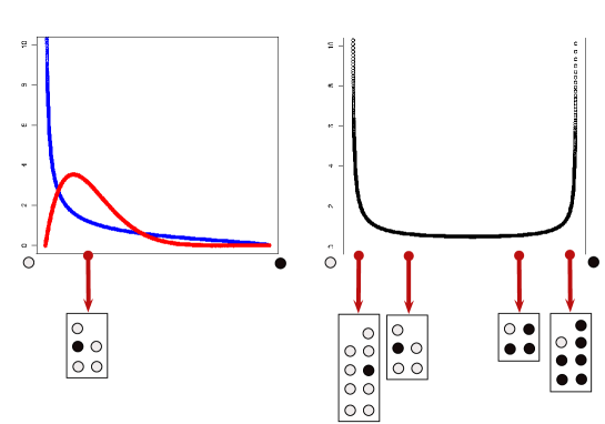
Figure 1: Documents generated from multinomials drawn from a Dirichlet distribution for both document (left) and background language models (right)

We now estimate the parameters of the document DCM $\bm{\alpha}_{d}$ using the observations from the actual document $d$. Given only one sample (i.e. the document) it is not possible to fully specify the maximum likelihood estimates of the document DCM. The maximum likelihood estimates of the multinomial inferred from one document will be equal to the expected value of the estimated DCM. Therefore, the maximum likelihood estimates of the multinomial from which the terms in the document were drawn (i.e. $c(t,d)/|d|$) will be proportional to the maximum likelihood estimates of the document DCM (i.e. $\bm{\hat{\theta}}_{d}\propto\bm{\hat{\alpha}}_{d}$). This is only true in the case where there is one sample.

Fig. 1 (left) shows this graphically for a simplified two-dimensional model that uses white and black balls to represent terms. The x-axis represents multinomials of varying parameter values. Points on the left-hand side of the x-axis represent multinomials where the probability of drawing a white ball are high, while points on the right-hand side of the x-axis represent multinomials where the probability of drawing a black ball are high. The Dirichlet distribution represents the likelihood of drawing these multinomials. In Fig 1 (left), the expectation of both of the two-dimensional Dirichlet distributions, shown by the red and blue curves, are equal and represent the multinomial (red arrow) inferred from the document.

Therefore, when we have only one multinomial (inferred from a document), we can only specify the location (expected multinomial) and not the shape (concentration parameter) of the DCM. In order to completely define the parameters of the document DCM, we also have to define the concentration $m_{d}=\sum_{{}_{t\in v}}{\alpha_{d_{t}}}$, which can be interpreted as the level of belief associated with the maximum likelihood estimates of the expected multinomial. Therefore, the initial parameters of the $|{v}|$-component document DCM are estimated as follows:

$$\bm{\hat{{\alpha}}}_{d}=m_{d}\cdot\bm{\hat{\theta}}_{d}=(m_{d}\cdot p(t_{1}|d),m_{d}\cdot p(t_{2}|d),....,m_{d}\cdot p(t_{|v|}|d))$$ (7)

where $p(t|d)=c(t,d)/|d|$ for all $t\in v$ and where $m_{d}$ is the initial mass that controls the burstiness of the document model. Although estimation of the parameters of the DCM using multiple data vectors is computationally expensive minka00, we can see that estimating the parameters of each document DCM is trivial if a suitable value for $m_{d}$ can be found.

Given that $m_{d}$ is the level of belief associated with the expected document multinomial $\bm{\hat{\alpha}}_{d}$, it would seem intuitive to aim to minimise this belief in the absence of evidence (an Occam’s razor type argument). A minimum setting can be arrived at by determining the minimum initial number of balls in the urn that could have generated the document. Given a document $d$, the minimum number of balls initially in the urn is the number of distinct coloured balls drawn. Therefore, we estimate the concentration parameter $m_{d}$ of the document DCM as $\hat{m}_{d}=|\vec{d}|$. This is the maximum amount of burstiness that is supported using this argument. In Fig. 1 (left) our estimate of $m_{d}$ for the document model is $m_{d}=2$, which leads to the shape of the Dirichlet in blue. Setting $m_{d}$ according to this parsimonious principle ensures that we have not over-fitted to our data.

4.5 Estimation of the Background DCM

For the DCM document models, there exists dependencies between successive occurrences of the same term in a document, and therefore, the estimation of the background DCM is more complex than for the multinomial distribution. In fact, in the entire collection, the only occurrences of the same term that are independent of each other are those in different documents. This leads to the introduction of a document boundary into the background DCM of the new language model, something that is lacking in the multinomial language model.

The estimation of a background DCM using all $n$ document vectors is, as mentioned previously, computationally expensive. However, elkan06 has shown that, for textual data, very close approximations to the maximum likelihood estimates of the DCM (via the EDCM) are proportional to $\sum_{j=1}^{n}I(c(t,d_{j})>0)$ for all $t\in v$, where $I$ is the indicator function. These approximations are accurate for textual data because most terms do not occur in all $n$ documents, and furthermore, it has been shown that the approximations make little difference to the effectiveness of the model for text-related tasks. It can be seen that this approximation relates to the number of documents in which a term occurs (i.e. the document frequency). Using an appropriate normalisation factor we obtain a probability estimate as follows:

$${p}(t|\bm{\hat{\theta^{\prime}}}_{c})=\frac{\sum_{j=1}^{n}I(c(t,d_{j})>0)}{\sum_{t^{\prime}\in v}df_{t^{\prime}}}=\frac{df_{t}}{\sum_{t^{\prime}\in v}df_{t^{\prime}}}=\frac{df_{t}}{\sum_{j=1}^{n}|\vec{d_{j}}|}$$ (8)

where $n$ is the number of documents in the collection and the numerator is the document frequency of a term. The normalisation factor can be re-written and comprises the summation of all document vectors in the collection so that $\sum_{t\in v}{p}(t|\bm{\hat{\theta^{\prime}}}_{c})=1$.

This probability distribution can be viewed as the expected multinomial drawn from the background EDCM. The estimates of the background DCM, which are approximately proportional to these probability estimates, are defined in a similar manner to the document DCM by introducing one concentration parameter $m_{c}$. This results in the following parameter estimates for the background DCM:

$$\bm{\hat{{\alpha}}}_{c}=(m_{c}\cdot{p}(t_{1}|\bm{\hat{\theta^{\prime}}}_{c}),m_{c}\cdot{p}(t_{2}|\bm{\hat{\theta^{\prime}}}_{c}),....,m_{c}\cdot{p}(t_{|v|}|\bm{\hat{\theta^{\prime}}}_{c}))$$ (9)

where $m_{c}$ is the belief in the expected value of the Dirichlet (i.e. ${p}(t|\bm{\hat{\theta^{\prime}}}_{c})$) and can be interpreted as a type of document word burstiness throughout the collection.

Fig. 1 (right) shows a graphical example of a two-dimensional background Dirichlet. As before, the x-axis determines parameter values of the multinomials, and the black curve shows the likelihood of drawing these multinomials. The four document samples shown in the figure exhibit high levels of burstiness as they contain a disproportionate number of balls of one specific colour. This is because areas of higher likelihood in Fig. 1 lead to multinomials with one component that contains most of the probability mass. The convex shape of this curve is due to a low $m_{c}$ concentration parameter, and therefore models high levels of word burstiness. Although the expectation of this over-dispersed two-dimensional Dirichlet has a low likelihood, it is nonetheless expected in the statistical sense. Essentially, the use of a DCM explains greater term-frequency variation in the $n$ documents in the collection.

4.6 Smoothing and Retrieval Models

We now present two smoothing methods which can be used to linearly combine $K$ multiple DCM models.

&

Figure 2: Document generation in the SPUD model for both types of smoothing

4.6.1 Linear Smoothing of Expected Multinomials

Conceptually, both the background and document DCM can be thought of as a Pólya urn. The first approach to smoothing treats each of these models as distinct Pólya urns. A document is generated by drawing with reinforcement, balls from the $K$ urns according to a certain probability. Essentially this smoothing approach linearly combines the expected values (multinomials) of the Dirichlets. This general smoothing approach is as follows:

$$p(d|\bm{\alpha}_{dm})=\sum^{K}_{i=1}\lambda_{i}\cdot p(d|{\bm{\alpha}}_{i})$$ (10)

where $\sum^{K}_{i=1}\lambda_{i}=1$ and ${\bm{\alpha}}_{i}$ is the $i^{th}$ DCM model. In this work we only linearly combine two models, the document DCM and the background DCM, and therefore the SPUD retrieval model using this smoothing approach is defined as follows:

$$\mathop{\mathbb{E}}[\bm{{\theta}}_{dm}|\bm{{\alpha}}_{dm}]=(1-\lambda_{jm})\cdot\bm{\theta}_{d}+\lambda_{jm}\cdot\bm{{\theta}^{\prime}}_{c}$$ (11)

where $\lambda_{jm}$ is the smoothing parameter and can be interpreted as the probability of selecting a term from the background DCM. We note that this formulation is identical to that of hiemstra98. Fig. 4.6 (left) shows the graphical model for the DCM language model with this type of linear smoothing (Jelinek-Mercer).

One of the main motivations for smoothing the document model with a background model is that the background model assigns mass to terms unseen in the document. Therefore, $\lambda_{jm}$ can be interpreted as the probability of drawing a previously unseen term from the background model, and $1-\lambda$ as the probability of drawing a previously seen term (i.e. a repeated term from the document). During the generation of the document $d$, at least $|\vec{d}|$ previously unseen terms were drawn. This leads to an estimate of $\hat{\lambda}_{jm}=|\vec{d}|/|d|$ as the probability of drawing an unseen term for that document model. This is the proportion of distinct terms in the document and is the estimate of drawing from the background multinomial $\bm{{\theta^{\prime}}_{c}}$. The SPUD retrieval model with this type of smoothing is denoted SPUD${}_{jm}$ and it has no free parameters. We note that the estimation of ${\lambda}_{jm}$ is not a consequence of the DCM model, and can therefore be applied to the multinomial language model that uses Jelinek-Mercer smoothing.

4.6.2 Linear Smoothing of DCMs

The second approach to smoothing uses a linear mixture of the DCM models. Conceptually, this approach to smoothing combines the contents of the $K$ urns into one single Pólya urn. A document is then generated by drawing with reinforcement from this single urn. This smoothing approach is a more complete Bayesian approach to smoothing and the parameters of the document model are as follows:

$$\bm{{\alpha}}_{dm}=\sum^{K}_{i=1}{\omega_{i}\cdot\bm{{\alpha}}_{i}}$$ (12)

where $\sum^{K}_{i=1}\omega_{i}=1$ and $\bm{{\alpha}}_{i}$ is the $i^{th}$ DCM language model. The $\omega$ parameters are linear mixing parameters that determine the relative weight of the DCM language models. It is worth noting that each of the DCMs has a concentration parameter $m_{i}$ which act to weight the vector appropriately. Given the document DCM and background DCM estimated previously, the smoothing is as follows:

$$\bm{\hat{\alpha}}_{dm}=(1-\omega)\cdot m_{d}\cdot\bm{\hat{\theta}}_{d}+\omega\cdot m_{c}\cdot\bm{\hat{\theta^{\prime}}}_{c}$$ (13)

where $\omega$ is the linear mixing parameter. Fig. 4.6 (right) shows the graphical model for this DCM mixture model. The expected multinomial drawn from this DCM mixture model is easily computed using the individual parameters of the DCM mixture model over the normalisation constant. This DCM mixture retrieval model is denoted SPUD${}_{dir}$ due to the mixing of the Dirichlets. Although it seems that the DCM mixture model still has two unknown parameters (i.e. $m_{c}$ and $\omega$), these can either be combined to form one single parameter, or $m_{c}$ can be estimated using numerical methods as outlined in the original work introducing the EDCM elkan06. We outline the details of these approaches in the next section.

5 Retrieval Model Implementation

In this section we outline the composition of the SPUD retrieval methods using both types of smoothing presented in the preceding section. We then present some retrieval intuitions that aid in understanding the retrieval aspects of the new model.

5.1 Retrieval Functions

Similarly to the implementation of the standard multinomial models zhai04, our approach can be computed efficiently using a summation that only involves terms common to both document and query. The SPUD${}_{jm}$ retrieval function using linear smoothing is as follows:

$$\bm{\textrm{SPUD}}_{jm}(q,d)=\sum_{t\in q}(log((1-\hat{\lambda}_{jm})\cdot\frac{c(t,d)}{|d|}+\hat{\lambda}_{jm}\cdot\frac{df_{t}}{\sum_{j}^{n}|\vec{d_{j}}|})\cdot c(t,q))$$ (14)

where $\hat{\lambda}_{jm}=|\vec{d}|/|d|$. This is rank equivalent to the following:

$$\bm{\textrm{SPUD}}_{jm}(q,d)=|q|\cdot log(\hat{\lambda}_{jm})+\sum_{t\in q\cap d}(log(1+\frac{(1-\hat{\lambda}_{jm})\cdot{c(t,d)}\cdot{\sum_{j}^{n}|\vec{d_{j}}|}}{{|\vec{d}|}\cdot{df_{t}}})\cdot c(t,q))$$ (15)

The SPUD${}_{dir}$ retrieval function can be computed in a somewhat similar form to the multinomial language model using Dirichlet prior smoothing as follows:

$$\bm{\textrm{SPUD}}_{dir}(q,d)=\sum_{t\in q}(log(\frac{(1-\omega)\cdot|\vec{d}|\cdot\frac{c(t,d)}{|d|}+{\omega\cdot m_{c}}\cdot\frac{df_{t}}{\sum_{j}^{n}|\vec{d_{j}}|}}{(1-\omega)\cdot|\vec{d}|+\omega\cdot m_{c}})\cdot c(t,q))$$ (16)

which is rank equivalent to the following:

$$\bm{\textrm{SPUD}}_{dir}(q,d)=|q|\cdot log(\frac{\mu^{\prime}}{\mu^{\prime}+|\vec{d}|})+\sum_{t\in q\cap d}(log(1+\frac{|\vec{d}|\cdot c(t,d)\cdot{\sum_{j}^{n}|\vec{d_{j}}|}}{\mu^{\prime}\cdot|d|\cdot df_{t}})\cdot c(t,q))$$ (17)

where $\mu^{\prime}$ is a combination of $\omega$ and $m_{c}$ as follows:

$$\mu^{\prime}=\frac{\omega}{1-\omega}\cdot m_{c}$$ (18)

As $\mu^{\prime}$ is the only parameter that has not been estimated so far, we now outline two approaches to finding suitable values for it. The first approach is to experimentally tune $\mu^{\prime}$ on training data in a similar manner to the Dirichlet prior smoothing parameter $\mu$ in the multinomial language model zhai01. Alternatively, $m_{c}$ can be estimated from the $n$ samples of observations using Newton’s method elkan06 as follows:

$$m_{c}^{new}=\frac{\sum_{j}^{n}|\vec{d_{j}}|}{\sum_{j}^{n}\psi(|d_{j}|+m_{c})-n\cdot\psi(m_{c})}$$ (19)

where $\psi(x)=\frac{d}{dx}log\Gamma(x)$ is the digamma function and $\Gamma$ is the gamma function. When estimating $m_{c}$ from the data using this method, $\omega$ is the parameter that requires experimental tuning. However, we expect that the one setting for the hyperparameter $\omega$ will perform robustly across many test collections. Experiments for both of these approaches to determining a suitable values the free parameters are are outlined in Section 6.4.

5.2 Length Normalisation and Document Boundary Retrieval Intuitions

We now examine some retrieval intuitions and existing hypotheses that help explain the differences between the SPUD retrieval functions and the multinomial retrieval functions. For most of the analysis in this section we focus on the best performing multinomial model (MQL${}_{dir}$) and its counterpart from the SPUD model (SPUD${}_{dir}$). robertson1994 outlined two hypotheses concerning the length of a document, namely the verbosity hypothesis and the scope hypothesis, which we now examine.

5.2.1 Verbosity Hypothesis

The verbosity hypothesis captures the intuition that some documents are longer than others simply because they are more verbose. Such documents do not describe more topics, they are simply more wordy. This hypothesis captures an aspect of document length that is independent of relevance. However, the initial description of this hypothesis robertson1994 does not outline any formal means of determining whether a particular retrieval function is consistent with the hypothesis. We now outline a retrieval constraint which helps to determine this.

LNC2*.

If document $d$ and $d^{\prime}$ are two documents, where $d^{\prime}$ is constructed by concatenating $d$ with itself $k$ times where $k>0$, and if $s(q,d)$ is the score returned from a retrieval function $s$ which is used to rank $d$ with respect to $q$, then $s(q,d)=s(q,d^{\prime})$.

This states that if a document is concatenated with itself any number of times, the retrieval score of that document should not change for a given query, and therefore it should not change rank. We call this constraint LNC2* as this is stricter than LNC2 outlined by fang04, which only states that $s(q,d)\leq s(q,d^{\prime})$. Essentially if a scoring function $s$ adheres to LNC2*, then we deem $s$ to be consistent with the verbosity hypothesis.

Consider a relevant document $d$ that is ranked in a certain position according to $s(q,d)$. If $d$ is replaced in the collection with $d^{\prime}$, $d^{\prime}$ should not be ranked lower than the initial document $d$. Therefore, $s(q,d^{\prime})$ should certainly not be less than $s(q,d)$ simply due to the verbosity of $d^{\prime}$. Now consider a non-relevant document $d$ of a given length. If $d$ is replaced in the collection with $d^{\prime}$, $d^{\prime}$ should not be ranked in a higher position than $d$ originally was. Therefore, given that we do not know the relevance of $d$ a priori, we argue that in general $s(q,d^{\prime})$ should not increase simply due to the increased verbosity of $d^{\prime}$.

The maximum likelihood estimate of a term in a document (i.e. $c(t,d)/|d|$) will not change if that document is concatenated with itself any number of times. However, in the multinomial language model using Dirichlet priors smoothing (MQL${}_{dir}$), LNC2* is only satisfied when $c(t,d)/|d|=cf_{t}/|c|$ which is not often the case. For this model, if there are many query-term matches in $d$, the more verbose document $d^{\prime}$ will nearly always be ranked higher than $d$ (i.e. $s(q,d^{\prime})>s(q,d)$), while if there are very few query-term matches in $d$ the verbose document $d^{\prime}$ will nearly always be ranked lower than $d$ (i.e. $s(q,d^{\prime})<s(q,d)$). However, if we examine the SPUD${}_{dir}$ method in Eq. (17), we can see that the document vector length $|\vec{d}|$ is used as one form of document length normalisation. The document vector length $|\vec{d}|$ will remain unchanged for the concatenated document $d^{\prime}$, and therefore $\bm{\textrm{SPUD}}_{dir}(q,d)=\bm{\textrm{SPUD}}_{dir}(q,d^{\prime})$.

In general the multinomial model not only over-promotes recurrences of query terms but over-penalises recurrences of non-query terms in a given document. Fig. 3 (left) shows the increase in weight as the term-frequency increases for both MQL${}_{dir}$ and SPUD${}_{dir}$. We can see that MQL${}_{dir}$ gives a greater weight to terms with higher frequencies than SPUD${}_{dir}$. This is because the aspect of document length that is affected as term-frequency increases is different for both retrieval functions. It is important that term-frequency is analysed considering the change in document length that an increase in term-frequency brings about. Fig. 3 (right) also shows the penalisation due to recurrences of non-query terms for both MQL${}_{dir}$ and SPUD${}_{dir}$. We can see that MQL${}_{dir}$ penalises recurrences of non-query terms more than SPUD${}_{dir}$. In the SPUD${}_{dir}$ function, recurrences of the same non-query term will always decrease the score of a document due to more off-topic verbosity.

$\begin{array}[]{c c}\includegraphics[height=113.81102pt,width=142.26378pt]{./analysis/tf-eps-converted-to}&\includegraphics[height=113.81102pt,width=142.26378pt]{./analysis/scope-eps-converted-to}\end{array}$

Figure 3: Change in weight as term-frequency increases for MQL${}_{dir}$ and SPUD${}_{dir}$ in a document that initially contains 100 distinct terms (left). Change in weight as recurring non-query terms are added to a document that initially contains 100 distinct terms (right).

Interestingly, it can be seen that the $\bm{\textrm{SPUD}}_{dir}$ formula in Eq. (17) contains the ratio between the term-frequency $c(t,d)$ and the average term-frequency in the document $|d|/|\vec{d}|$. This average term-frequency normalisation idea was first proposed by singhal96, but in general was not shown to improve retrieval effectiveness substantially until recent research paik:13. It is this part of the $\bm{\textrm{SPUD}}_{dir}$ retrieval model that deals specifically with the verbosity hypothesis, while the document length normalization component, the left-hand side of Eq. (17), deals with the scope hypothesis by replacing the original document length with the document vector length. We now discuss this further.

5.2.2 Scope Hypothesis

The scope hypothesis captures the alternative intuition that documents may be longer because they cover many different topics. It has been noted in the original work regarding the scope hypothesis robertson1994 that many Newswire documents in the original TREC corpora seemed as if they consisted of multiple different news articles concatenated together. In the multinomial language model there is no difference in the normalisation applied when a term occurs for the first time (i.e. an increase in scope) as opposed to when a term repeats itself (i.e. an increase in verbosity). This difference is modelled in the new SPUD language models and can be viewed as being modelled separately for SPUD${}_{dir}$. In Eq. (17), we can see that the factor $|q|\cdot log(u^{\prime}/(u^{\prime}+|\vec{d}|))$ leads to a penalisation only for the occurrence of distinct terms (i.e. when the scope broadens). If the term re-occurs, it is not penalised by the part of the retrieval function which deals with scope.

For the SPUD${}_{dir}$ model, adding a non-query term into a document for the first time will lead to penalisation by the normalisation aspect that deals with scope. However, it should be noted that the verbosity aspect of a document is also affected by the addition of previously unseen non-query terms and this actually promotes existing query-terms. Therefore, the overall document score does not necessarily decrease when a new non-query term is added.

In the SPUD${}_{dir}$ model, the magnitude of the document score penalisation for the first occurrence of a non-query term is quite similar to the penalisation applied by MQL${}_{dir}$ (See Fig. 3), but recurrences are not penalised as much. Given these observations, we hypothesise that the SPUD${}_{dir}$ retrieval method does not penalise long documents as much as MQL${}_{dir}$. Recent research has studied the over penalisation of long documents by many retrieval functions including MQL${}_{dir}$ lv11. They built upon work by singhal96 which showed that most ranking functions retrieve long documents with a likelihood less than their likelihood of relevance. We replicate that analysis by binning according to length, relevant documents and then estimating the probability that a document occurs in a given bin (length) given that it is relevant. The same procedure is applied to retrieved documents where a document is deemed retrieved if it occurs in the top 1000 documents of the ranked list. We use the same binning strategy as lv11 (i.e. 5000) and compared the MQL${}_{dir}$ and SPUD${}_{dir}$ retrieval functions. The aspect of length used in this analysis is that of the number of word tokens in the document (i.e. $|d|$).

$\begin{array}[]{c c c}\includegraphics[height=113.81102pt,width=142.26378pt]{./analysis/prob_rel_wt10g_title-eps-converted-to}&\includegraphics[height=113.81102pt,width=142.26378pt]{./analysis/prob_rel_wt10g_desc-eps-converted-to}\\ \end{array}$

Figure 4: Probability of retrieval/relevance for MQL${}_{dir}$ and SPUD${}_{dir}$ methods for trec-9/10 collection for short queries (left) and medium length queries (right).

Fig. 4 shows the probability of relevance (in black) and the probability of retrieval for both MQL${}_{dir}$ (in blue) and SPUD${}_{dir}$ (in red) on one collection. Firstly, we note that the trends are consistent with the previous approaches singhal96; lv11. Furthermore, we can see that longer documents have a higher likelihood of being retrieved by the SPUD${}_{dir}$ approach compared to the MQL${}_{dir}$ approach. This confirms our intuitions that the SPUD${}_{dir}$ model does not penalise long documents as much as MQL${}_{dir}$ and that we would expect the SPUD method to retrieve long documents with a probability closer to their likelihood of relevance. We investigate this further in the experimental section (Section 6.5).

5.2.3 Background model

Sample collection of four documents and two terms docs $t_{1}$ $t_{2}$ $d_{1}$ 8 2 $d_{2}$ 0 1 $d_{3}$ 0 3 $d_{4}$ 0 1

The new background model in the SPUD brings about some other interesting retrieval characteristics. Given the sample collection in Table 5.2.3 of four documents and two terms ($t_{1}$ and $t_{2}$), we might wish to determine the most likely one term string, $q=\{t_{1}\}$ or $q=\{t_{2}\}$, generated from the background model. If we assume a multinomial background model estimated using maximum likelihood, then $p(t_{1}|\bm{\hat{\theta}}_{c})=8/15$ and $p(t_{2}|\bm{\hat{\theta}}_{c})=7/15$, suggesting that term $q=\{t_{1}\}$ is the more likely. However, intuitively we see that the high frequency of ${t_{1}}$ in document $d_{1}$ is unduly biasing the estimates, especially as term ${t_{1}}$ only appears in one document. Term ${t_{2}}$ occurs in all of the documents, and therefore, is a word used more widely in the collection (possibly by more authors in general). The SPUD model takes the document boundary into account yielding estimates of $p(t_{1}|\bm{\hat{\theta^{\prime}}}_{c})=1/5$ and $p(t_{2}|\bm{\hat{\theta^{\prime}}}_{c})=4/5$ respectively. This probability is similar to that proposed in one of the first language modelling approaches hiemstra98, and has recently been re-examined as being potentially theoretically valid roelleke12.

$\begin{array}[]{c c c}\includegraphics[height=113.81102pt,width=142.26378pt]{./intuitions/idf-eps-converted-to}&\end{array}$

Figure 5: idf and global weightings derived from the SPUD model

As seen in this toy example, the proposed model uses the document frequency in its approximation for the parameters of the background DCM. Furthermore, the normalisation component used in the background model can be written as $\sum_{j}^{n}|\vec{d_{j}}|=n\cdot|\vec{d}|_{avg}$, where $|\vec{d}|_{avg}$ is the average document vector length. Therefore, in the SPUD${}_{dir}$ retrieval formula, the weight assigned to a query-term that occurs in a document comprises of the following factor as per the right-hand side of Eq. (17):

$$\sum_{t\in q\cap d}log(1+\delta\cdot\frac{n}{df_{t}})\cdot c(t,q)$$ (20)

where $\delta=|\vec{d}|\cdot|\vec{d}|_{avg}\cdot c(t,d)/(\mu^{\prime}\cdot|d|)$. We can see that this factor can be viewed as a new family of idf. Unlike the traditional idf measure, this factor is document-length, document-vector-length, and term-frequency specific. We have found that $\delta$ typically ranges from $0.05$ to $0.5$ for query terms on many of the collections used in this work. Fig. 5 shows the weight assigned by idf and by Eq. (20) as the document frequency changes. This suggests that the global weighting factor in our new approach is closely related to idf. This crude comparison by no means validates the traditional idf in a theoretical perspective, nevertheless it does present a theoretical means by which aspects of both term-frequency and document frequency combine in one model. In contrast, the multinomial language modelling approach treats terms that are completely independent of each other, written by different authors on different topics, similarly to terms that are highly dependent on each other (e.g. terms that are repeated, possibly due to association, in a document written by one author on a particular topic). Discovering a theoretical justification for the combination of both term-frequency and idf is problematic as they appear to lie in different event spaces. The preferential attachment captured in the SPUD model is a promising generative theory justifying tf-idf type schemes.

A practical consideration is whether there is substantial difference between the probability of a term given either background model (multinomial or DCM) when estimated from data. Therefore, we estimated the background probability of seeing a term for both models for all query terms on one of the test collections used in our experiments. We analysed 1530 query-terms from the trec-9/10 test collection and we found a high linear correlation (0.954) between the estimated probabilities for the terms. This is to be expected as the probabilities are fundamentally capturing similar information about a term. However, there are examples where the estimated probabilities of actual query-terms are quite different. Table 5.2.3 shows the top and bottom 10 terms when ranked according to the ratio of their probabilities (i.e. $p(t|\bm{\alpha}_{c})/p(t|\bm{\theta}_{c})$). The bottom 10 terms show those that the background multinomial gives a much higher probability to when compared to the background DCM. It is interesting that the term el, which has much higher probability in the multinomial model, is a stopword from a different language. This receives a relatively high probability estimate from a multinomial because it appears many times, but receives a much lower probability estimate from the background DCM because many of these appearances come from few documents (i.e. the term is quite bursty). The background DCM regards these terms as less general than the multinomial, as the occurrences have actually occurred in fewer documents. Conversely, the top 10 terms show those that the multinomial model has estimated as less general but which the background DCM has estimated as being more general. These terms are less bursty but have occurred in many documents in the collection.

Therefore, given that there exists query-terms where the probability of occurrence under our new model is quite different, we would expect this to impact retrieval effectiveness. We evaluate the effect that the new document normalisation and background model have on retrieval effectiveness separately in Section 6.5.

Ratio of estimated query-term probabilities of DCM to multinomial model ($p(t|\bm{\alpha}_{c})/p(t|\bm{\theta}_{c})$) for a number of query-term on trec-9/10 terms Bottom 10 Top 10 1 vike 0.3461802368 funnel-shap 2.0327764077 2 el 0.3910938927 undergon 1.9616724275 3 cancer 0.4098663257 pejor 1.9517391904 4 patient 0.415028517 tartin 1.9495633384 5 cell 0.4180174157 superstiti 1.9149743114 6 student 0.4289654263 gynt 1.9071815267 7 drug 0.4726560064 interest 1.8928123508 8 system 0.4950172629 unsuccess 1.8803346212 9 law 0.5064728539 work 1.8709780476 10 infect 0.51433562 run-awai 1.8666031964

6 Experiments

In this section we outline the experiments used to evaluate the new SPUD methods. We first outline the experimental design and methodology, before presenting the experiments.

6.1 Experimental Design

We carry out four experiments to evaluate different aspects of the new SPUD query likelihood models. The first experiment evaluates the retrieval effectiveness of the new SPUD retrieval methods against a number of baselines. The second experiment evaluates the robustness of the tuning parameters in the SPUD retrieval methods. The third experiment presents an analysis of the retrieval intuitions outlined in the preceding section. Finally, we evaluate the best SPUD retrieval method when incorporating it into a pseudo-relevance feedback framework.

6.2 Datasets

Table 6.2 shows the characteristics of the TREC test collections used in the experiments. We use a wide variety of TREC collections that are of varying sizes and include collections of Web documents, Newswire articles, and medical abstracts. In our experiments we evaluate short keyword queries (2-3 terms) consisting of the title field of the trec topic, medium queries (6-10 terms) consisting of both the title and description fields of the topics, and long verbose queries (10-30 terms) consisting of the title, description, and narrative fields of the topic. We remove standard stopwords and apply stemming using Porter’s stemmer. It is worth noting that the ohsumed test collection contains only description length queries (i.e. medium length queries), while there are only title length queries available for the mq-07 and mq-08 test collections.

Test Collection Details query length label collection # docs # topics topic range short medium long (title) (title+desc) (title+desc+narr) ohsu ohsumed 293,856 63 001-63 n/a 5.0 n/a robust-04 fr, ft,la, fbis 528,155 250 301-450, 601-700 2.5 10.3 31.4 trec-8 wt2g 221,066 50 401-450 2.4 9.0 27.5 trec-9/10 wt10g 1,692,096 100 451-550 2.6 9.3 24.3 gov2 gov2 25,205,179 150 701-850 2.8 8.6 33.3 mq-07 gov2 25,205,179 1778 1-10k 3.1 n/a n/a mq-08 gov2 25,205,179 784 10k - 20k 3.7 n/a n/a

6.3 Retrieval Effectiveness

The first experiment evaluates the retrieval effectiveness of the SPUD model against its counterpart, the standard multinomial query likelihood language model. We compare the SPUD${}_{jm}$ retrieval function against the multinomial query likelihood function with Jelinek-Mercer smoothing (MQL${}_{jm}$). We tune the MQL${}_{jm}$ function for each set of queries to optimise mean average precision (MAP) on each test collection where the parameter space $\pi_{jm}\in\{0.1,0.2,...,0.9,1.0\}$. Therefore, we are confident that the effectiveness of the MQL${}_{jm}$ retrieval function is close to its optimal on each collection. On the other hand, we do not tune SPUD${}_{jm}$ as it has no free-parameters.

We compare the SPUD${}_{dir}$ retrieval function against its counterpart, the multinomial query likelihood function with Dirichlet-prior smoothing (MQL${}_{dir}$). Similarly, we tune the MQL${}_{dir}$ function to optimise MAP on each test collection where the parameter space $\mu\in\{250,500,...,2250,2500\}$. We report the effectiveness of the SPUD${}_{dir}$ retrieval function for same parameter setting as MQL${}_{dir}$ (i.e. $\mu=\mu^{\prime}$). This evaluation favours MQL${}_{dir}$ as SPUD${}_{dir}$ may not be tuned optimally.

We also use the DCM-L-T retrieval function xu08 which has a tuning parameter $\gamma$. We tuned $\gamma$ for each set of queries on each collection over the parameter space $\gamma\in\{0.1,0.2,...,0.9,1.0\}$.

6.3.1 Retrieval Effectiveness Results

Tables 6.3.1 and 6.3.1 show the retrieval effectiveness (MAP and NDCG@20) of MQL${}_{jm}$ compared to SPUD${}_{jm}$, and MQL${}_{dir}$ compared to SPUD${}_{dir}$ for short title queries (2-3 terms on average). We can see that on most of the test collections the SPUD retrieval methods demonstrate a significant increase in effectiveness for both MAP and NDCG@20 over their corresponding MQL methods.

MAP of SPUD models vs MQL models ($\blacktriangle$ means two-sided t-test $p<0.01$, $\triangle$ means $p<0.05$) and SPUD models vs DCM-L-T ($\bullet$ means two-sided t-test $p<0.01$ compared to DCM-L-T, $\circ$ means $p<0.05$ compared to DCM-L-T). short queries robust-04 trec-8 trec-9/10 gov2 mq-07 mq-08 DCM-L-T 0.248 0.306 0.187 0.288 0.409 0.413 MQL${}_{jm}$ 0.231 0.246 0.135 0.245 0.396 0.419 SPUD${}_{jm}$ 0.236 0.255 0.154$\triangle$ 0.276$\blacktriangle$ 0.411$\blacktriangle$ 0.430$\blacktriangle$ MQL${}_{dir}$ 0.247 0.308 0.192 0.303 0.420 0.427 SPUD${}_{dir}$ 0.252$\blacktriangle$ 0.319$\triangle$ 0.200$\triangle$ 0.314$\blacktriangle\bullet$ 0.431$\blacktriangle\bullet$ 0.445$\blacktriangle\circ$

NDCG@20 of SPUD models vs MQL models ($\blacktriangle$ means two-sided t-test $p<0.01$, $\triangle$ means $p<0.05$) and SPUD models vs DCM-L-T ($\bullet$ means two-sided t-test $p<0.01$ compared to DCM-L-T, $\circ$ means $p<0.05$ compared to DCM-L-T). short queries robust-04 trec-8 trec-9/10 gov2 mq-07 mq-08 DCM-L-T 0.423 0.449 0.298 0.455 0.465 0.495 MQL${}_{jm}$ 0.385 0.356 0.220 0.379 0.458 0.495 SPUD${}_{jm}$ 0.398 $\blacktriangle$ 0.384$\triangle$ 0.243$\triangle$ 0.418$\blacktriangle$ 0.474$\triangle$ 0.503 MQL${}_{dir}$ 0.423 0.466 0.309 0.470 0.488 0.500 SPUD${}_{dir}$ 0.432 $\blacktriangle$ 0.477 0.322 0.492$\blacktriangle\bullet$ 0.500$\blacktriangle\circ$ 0.513$\blacktriangle\circ$

Tables 6.3.1 and 6.3.1 show the retrieval effectiveness (MAP and NDCG@20) of MQL${}_{jm}$ compared to SPUD${}_{jm}$, and MQL${}_{dir}$ compared to SPUD${}_{dir}$ for medium length queries (6-10 terms on average). Again we can see that on most of the test collections the SPUD models demonstrate an increase in effectiveness for both MAP and NDCG@20. All of these increases are significant in the case of SPUD${}_{dir}$. For long queries (10-30 terms on average) we see a similar trend. A point worth emphasising is that the increases in effectiveness are also present at the top of the ranked lists as demonstrated by NDCG@20.

The SPUD${}_{dir}$ approach outperforms the previous DCM relevance-based model (DCM-L-T) on most test collections. We have found that the DCM-L-T performs similarly to MQL${}_{dir}$ for short queries on some of the smaller collections, but we find that the DCM-L-T approach performs quite poorly on the larger gov2, mq-07, and mq-08 test collections and for all medium and long queries. Statistical significance tests (using a two-sided t-test indicated by $\circ$ and $\bullet$) show that the best performing SPUD model (SPUD${}_{dir}$) outperforms the DCM-L-T approach on some collections for short queries and consistently outperforms a tuned DCM-L-T approach for longer queries. We discuss some possible reasons for these results in Section 7.1.

MAP of SPUD models vs MQL models ($\blacktriangle$ means two-sided t-test $p<0.01$, $\triangle$ means $p<0.05$) and SPUD models vs DCM-L-T ($\bullet$ means two-sided t-test $p<0.01$ compared to DCM-L-T, $\circ$ means $p<0.05$ compared to DCM-L-T). medium length queries robust-04 trec-8 trec-9/10 gov2 ohsu DCM-L-T 0.266 0.296 0.181 0.256 0.255 MQL${}_{jm}$ 0.277 0.283 0.191 0.276 0.239 SPUD${}_{jm}$ 0.280 0.291 0.203$\blacktriangle\circ$ 0.299$\blacktriangle\bullet$ 0.248$\triangle$ MQL${}_{dir}$ 0.281 0.325 0.238 0.315 0.253 SPUD${}_{dir}$ 0.289$\blacktriangle\bullet$ 0.347$\blacktriangle\bullet$ 0.247$\blacktriangle\bullet$ 0.329$\blacktriangle\bullet$ 0.270$\blacktriangle\bullet$

NDCG@20 of SPUD models vs MQL models ($\blacktriangle$ means two-sided t-test $p<0.01$, $\triangle$ means $p<0.05$) and SPUD models vs DCM-L-T ($\bullet$ means two-sided t-test $p<0.01$ compared to DCM-L-T, $\circ$ means $p<0.05$ compared to DCM-L-T). medium length queries robust-04 trec-8 trec-9/10 gov2 ohsu DCM-L-T 0.435 0.436 0.318 0.401 0.396 MQL${}_{jm}$ 0.455 0.412 0.329 0.431 0.397 SPUD${}_{jm}$ 0.456 0.440$\triangle$ 0.344$\triangle\bullet$ 0.463$\blacktriangle\bullet$ 0.391 MQL${}_{dir}$ 0.465 0.478 0.393 0.484 0.399 SPUD${}_{dir}$ 0.479$\blacktriangle\bullet$ 0.500$\blacktriangle\bullet$ 0.403$\triangle\bullet$ 0.502$\blacktriangle\bullet$ 0.415$\blacktriangle\circ$

MAP of SPUD models vs MQL models ($\blacktriangle$ means two-sided t-test $p<0.01$, $\triangle$ means $p<0.05$) and SPUD models vs DCM-L-T ($\bullet$ means two-sided t-test $p<0.01$ compared to DCM-L-T, $\circ$ means $p<0.05$ compared to DCM-L-T). long queries robust-04 trec-8 trec-9/10 gov2 DCM-L-T 0.239 0.225 0.181 0.235 MQL${}_{jm}$ 0.284 0.269 0.211 0.265 SPUD${}_{jm}$ 0.288$\triangle\bullet$ 0.269 $\bullet$ 0.206 $\circ$ 0.285 $\blacktriangle\bullet$ MQL${}_{dir}$ 0.283 0.283 0.248 0.296 SPUD${}_{dir}$ 0.296$\blacktriangle\bullet$ 0.314$\blacktriangle\bullet$ 0.254 $\bullet$ 0.323 $\blacktriangle\bullet$

NDCG@20 of SPUD models vs MQL models ($\blacktriangle$ means two-sided t-test $p<0.01$, $\triangle$ means $p<0.05$) and SPUD models vs DCM-L-T ($\bullet$ means two-sided t-test $p<0.01$ compared to DCM-L-T, $\circ$ means $p<0.05$ compared to DCM-L-T). long queries robust-04 trec-8 trec-9/10 gov2 DCM-L-T 0.404 0.346 0.318 0.400 MQL${}_{jm}$ 0.469 0.430 0.354 0.535 SPUD${}_{jm}$ 0.476 $\bullet$ 0.431 $\bullet$ 0.356 $\bullet$ 0.541 $\bullet$ MQL${}_{dir}$ 0.467 0.446 0.406 0.572 SPUD${}_{dir}$ 0.483$\blacktriangle\bullet$ 0.475$\triangle\bullet$ 0.409 $\bullet$ 0.599 $\blacktriangle\bullet$

$\begin{array}[]{c c c}\includegraphics[height=99.58464pt,width=113.81102pt]{./analysis/trec_4_5_title-eps-converted-to}&\includegraphics[height=99.58464pt,width=113.81102pt]{./analysis/trec_4_5_desc-eps-converted-to}&\includegraphics[height=99.58464pt,width=113.81102pt]{./analysis/trec_4_5_narr-eps-converted-to}\\ \includegraphics[height=99.58464pt,width=113.81102pt]{./analysis/wt10g_title-eps-converted-to}&\includegraphics[height=99.58464pt,width=113.81102pt]{./analysis/wt10g_desc-eps-converted-to}&\includegraphics[height=99.58464pt,width=113.81102pt]{./analysis/wt10g_narr-eps-converted-to}\\ \end{array}$

Figure 6: Average precision of all short, medium, and long queries for MQL${}_{dir}$ vs SPUD${}_{dir}$ on robust-04 dataset (top) and trec-9/10 (bottom)

Fig.6 shows the performance of MQL${}_{dir}$ vs SPUD${}_{dir}$ for each query on two separate test collections. This query specific analysis indicates that SPUD${}_{dir}$ is robust on all ranges of queries (from easy to difficult). For longer queries on the robust-04 dataset, there are one or two high performing queries which drop over 0.1 in average precision. However, in general there are very few queries which severely under perform compared to MQL${}_{dir}$. On the trec-9/10 web documents, the increase in performance is stable across all types of queries for all query lengths.

6.4 Robustness

The second experiment evaluates the robustness of the SPUD models with respect to different parameter settings. In addition, we evaluate the retrieval effectiveness of the SPUD${}_{dir}$ model when the parameter $\mu^{\prime}$ is derived from the estimated parameter $m_{c}$ using Newton’s method elkan06.

6.4.1 Robustness Results

Fig. 7 shows the performance of MQL${}_{jm}$ over different tuning parameter values (i.e. $\pi_{jm}$) and the performance of the SPUD${}_{jm}$ model. We can see that SPUD${}_{jm}$, which has no free parameters, outperforms SPUD${}_{jm}$ over all parameter values. This trend is consistent on all test collections used here.

$\begin{array}[]{c c }\includegraphics[height=113.81102pt,width=128.0374pt]{./tuning/trec_4_5_linear_title-eps-converted-to}&\includegraphics[height=113.81102pt,width=128.0374pt]{./tuning/wt10g_linear_title-eps-converted-to}\end{array}$

Figure 7: Robustness comparison of MQL${}_{jm}$ and SPUD${}_{jm}$ on robust-04 (left) and trec-9/10 (right) for short queries

For the SPUD${}_{dir}$ function, we can estimate $m_{c}$ using Newton’s method as outlined in Eq. (19) given the $n$ documents as data. We found that an initial value of $m_{c}=200$ was suitable so that the process converged within 20 iterations. This computation can be done off-line and we used the resulting setting of $m_{c}$ to estimate $\mu^{\prime}$ by tuning the hyperparameter $\omega$ to a fixed value. We set $\omega=0.8$ which is demonstrated in Fig. 8 as a reasonable setting. Fig. 8 shows the performance (MAP) of the SPUD${}_{dir}$ model for different values of $\omega$ when $m_{c}$ is estimated using Newton’s method. The relationship between $\omega$ and $\mu^{\prime}$ in Eq. (18) essentially suggests that $\mu^{\prime}=4\cdot m_{c}$ is a suitable parameter value for $\mu^{\prime}$. Although $m_{c}$ is the only parameter that is expensive to estimate in the SPUD${}_{dir}$ model, it is practically feasible to do so offline. When the parameter $\mu^{\prime}$ is computed in this way (i.e. $\mu^{\prime}=4\cdot m_{c}$), we denote this SPUD${}_{est_{\mu^{\prime}}}$ in the experimental results and figures that follow.

$\begin{array}[]{c }\includegraphics[height=128.0374pt,width=156.49014pt]{./tuning/omega_tuning-eps-converted-to}\end{array}$

Figure 8: Tuning of $\omega$ in SPUD${}_{dir}$ on robust-04 (short), trec-8 (short), and ohsu (medium) collections when $m_{c}$ is estimated using Eq. (19)

Fig. 9 shows the performance of MQL${}_{dir}$, SPUD${}_{dir}$, and SPUD${}_{est_{\mu^{\prime}}}$ over different parameter settings on a number of test collections. We can see that SPUD${}_{dir}$ outperforms MQL${}_{dir}$ over all parameter values. We can see that the parameter $\mu^{\prime}$ is as robust as the parameter $\mu$, as it tends to follow the same trend.

$\begin{array}[]{c c }\includegraphics[height=113.81102pt,width=128.0374pt]{./tuning/trec_4_5_dir_title-eps-converted-to}&\includegraphics[height=113.81102pt,width=128.0374pt]{./tuning/wt10g_dir_title-eps-converted-to}\end{array}$

Figure 9: Robustness of SPUD${}_{dir}$ and MQL${}_{dir}$ over different values of the tuning parameter $\mu$ (or $\mu^{\prime}$) on robust-04 (short) and trec-9/10 (short) respectively

More importantly we see that near optimal effectiveness can usually be achieved by using the automatically estimated value of $m_{c}$ found using Newton’s method. This is rather encouraging as it means that the setting of $\omega=0.8$ is robust and that we can effectively and safely eliminate from SPUD${}_{dir}$ the free parameters. In particular, this automatic optimal estimation can be seen when we examine in Fig. 9 the trec-9/10 collection (which contains long Web documents) and the robust-04 collection (which has shorter documents). For the robust-04 collection, the retrieval effectiveness decreases sharply when $\mu^{\prime}$ becomes greater than 1000. On the other hand, for the trec-9/10 the effectiveness is more stable when $\mu^{\prime}$ is greater than 1000. One probable reason for this is that the average length of the documents in those collections is very different. However, the automatically estimated SPUD${}_{est_{\mu^{\prime}}}$ is close to optimal on both collections.

Table 6.4.1 reinforces this observation. Table 6.4.1 shows the characteristics of the average length of documents in the collections and the value of $m_{c}$ that is estimated on each collection. We can also see that $m_{c}$ is correlated with the lengths of documents in the collections. Furthermore, in the same table we can see that close to the optimal effectiveness is possible by setting $\omega=0.8$ for SPUD${}_{est_{\mu^{\prime}}}$. This is because $m_{c}$ is essentially performing the tuning on a per collection basis. The parameter $m_{c}$ has a very intuitive interpretation as the initial mass of the background Pólya urn.

MAP comparison of SPUD${}_{dir}$ model for well-tuned $\mu^{\prime}$ and SPUD${}_{est_{\mu^{\prime}}}$ which uses an automatically estimated value of $\mu^{\prime}$ robust-04 trec-8 trec-9/10 ohsu gov2 mq-07 mq-08 $|\vec{d}|_{avg}$ 162 242 157 68 181 181 181 $|d|_{avg}$ 265 558 344 104 529 529 529 $\hat{m_{c}}$ 258 421 326 112 234 234 234 $\hat{u^{\prime}}=4\cdot\hat{m_{c}}$ 1034 1688 1308 448 936 936 936 short queries SPUD${}_{dir}$ 0.252 0.319 0.200 n/a 0.314 0.431 0.445 SPUD${}_{est_{\mu^{\prime}}}$ 0.249 0.320 0.199 n/a 0.314 0.429 0.443 medium queries SPUD${}_{dir}$ 0.289 0.347 0.247 0.270 0.332 n/a n/a SPUD${}_{est_{\mu^{\prime}}}$ 0.287 0.344 0.246 0.270 0.329 n/a n/a long queries SPUD${}_{dir}$ 0.296 0.314 0.254 n/a 0.323 n/a n/a SPUD${}_{est_{\mu^{\prime}}}$ 0.295 0.307 0.255 n/a 0.322 n/a n/a

6.5 Analysis of Retrieval Model Aspects

In this third experiment we aim to evaluate the retrieval effectiveness of the new background model (i.e. $\bm{\alpha}_{c}$) and the new smoothing methods in the SPUD model separately in a piece-wise fashion. We gradually adapt parts of the multinomial query likelihood functions until the SPUD retrieval functions are comprised. The experiment pinpoints the parts of the SPUD retrieval functions that lead to changes in retrieval effectiveness. This piece-wise adaptation provides evidence that the individual retrieval intuitions outlined in Section 5.2 are valid. Furthermore, we conduct an analysis of the retrieval characteristics of the best performing methods.

6.5.1 Results of the Analysis of Retrieval Model Aspects

Table 6.5.1, which also contains a column for a hybrid model, outlines the parameter values for the functions used in this experiment. Essentially, this hybrid retrieval function differs from the SPUD retrieval functions only in the fact that it uses different parameter estimates for $\lambda_{jm}$ and $m_{d}$ that effect the smoothing for SPUD${}_{jm}$ and SPUD${}_{dir}$ respectively. The changes to these parameter estimates makes the hybrid model closer to the multinomial retrieval functions. The only difference between the MQL and $hybrid$ model is that $hybrid$ uses the expected multinomial of the background DCM (i.e. $\bm{\theta}_{c}^{\prime}$ in Eq. 8) as its background model.

Decomposition of Retrieval Functions MQL $hybrid$ SPUD Smoothing Colour Multinomial DCM DCM Jelinek-Mercer (jm) Blue $\pi_{jm}=0.2$ $\lambda_{jm}=0.2$ $\lambda_{jm}=|\vec{d}|/|d|$ Dirichlet (dir) Red $\mu=2000$ $\mu^{\prime}=2000$, $m_{d}=|d|$ $\mu^{\prime}=2000$, $m_{d}=|\vec{d}|$

$\begin{array}[]{c c c}\includegraphics[height=113.81102pt,width=142.26378pt]{./intuitions/wt2g_linear-eps-converted-to}&\includegraphics[height=113.81102pt,width=142.26378pt]{./intuitions/wt2g_dir-eps-converted-to}\\ \includegraphics[height=113.81102pt,width=142.26378pt]{./intuitions/wt10g_linear-eps-converted-to}&\includegraphics[height=113.81102pt,width=142.26378pt]{./intuitions/wt10g_dir-eps-converted-to}\end{array}$

Figure 10: Analysis of performance gains from different parts of the SPUD retrieval models for trec-8 (top) and trec-9/10 (bottom) for short, medium, and long queries. Models that use Jelinek-Mercer smoothing are on the left-hand, side while those that use Dirichlet smoothing are on the right-hand side.

Fig. 10 shows the effectiveness of the functions that use Jelinek-Mercer smoothing (left-hand side) and those that use a type of Dirichlet smoothing (right-hand side) on two test collections. In general, the use of the new background DCM model aids retrieval as we can see an increase in effectiveness for the $hybrid$ (in black) retrieval functions over the MQL functions (in blue). We note that the magnitude of the difference is small, and that in some cases the performance decreases slightly. In general, the introduction of a document boundary into the estimation of the background language model is more effective for SPUD${}_{dir}$ than for SPUD${}_{jm}$.

However, the different smoothing techniques introduced in the SPUD model yield a greater increase in performance i.e. when comparing the SPUD function (in red) to the $hybrid$ function (in black). The smoothing in the SPUD model, amongst other factors, affects document length normalisation and improves retrieval effectiveness substantially. The results in Fig. 10 demonstrate that the new retrieval characteristics brought about by both the background DCM and the document DCM positively influence retrieval effectiveness. The results of these experiments further validate the use of the DCM as a more plausible document model than the multinomial. This is because the changes to the query-likelihood retrieval method that the new background and new document model bring about, increase the retrieval effectiveness for SPUD${}_{dir}$ method over MQL.

Previously in Section 5.2.2 we analysed the lengths of documents retrieved in the top 1000 documents by both MQL${}_{dir}$ and SPUD${}_{dir}$. We found that SPUD${}_{dir}$ was more likely to retrieve longer documents. We now look at the length characteristics of the top 20 documents returned per query by both SPUD${}_{dir}$ and MQL${}_{dir}$ to determine if the differences in length are correlated with increased performance in terms of NDCG@20. Firstly Fig.11 confirms that on average SPUD${}_{dir}$ retrieves documents with a longer vector length than MQL${}_{dir}$ in the top 20. Table 6.5.1 shows the correlation between the differences in average length and the differences in NDCG in the top 20 documents across a number of representative test collections. We report a small but insignificant correlation between the increase in average vector length and query effectiveness (as measured by NDCG@20). Although this correlation analysis is somewhat inconclusive, we can confirm that on average SPUD${}_{dir}$ retrieves documents with a longer vector length (i.e. greater number of distinct terms), and that the overall evidence seems to suggest that this is leading to increase effectiveness.

$\begin{array}[]{c c c}\includegraphics[height=113.81102pt,width=142.26378pt]{./analysis/vector_length_wt2g-eps-converted-to}&\includegraphics[height=113.81102pt,width=142.26378pt]{./analysis/vector_length_gov2-eps-converted-to}\\ \end{array}$

Figure 11: Difference in average vector length of the top 20 returned documents for SPUD${}_{dir}$ and MQL${}_{dir}$ on trec-8 (left) and gov2 (right) web collections for short queries.

Linear correlation of $\Delta$ average document length in top 20 and $\Delta$ NDCG@20 over short queries sets for Web collections avg_len trec-8 trec-9/10 gov2 $|d|$ 0.0525 0.0462 -0.0161 $\vec{|d|}$ 0.0838 0.0622 0.0216

6.6 Pseudo-Relevance Feedback

Finally, we evaluate the SPUD model in a pseudo-relevance feedback setting. Pseudo-relevance feedback is a useful approach for expanding short queries when the user has not entered a sufficiently long query. In essence, the pseudo-relevance model is responsible for the selection and weighting of candidate expansion query-terms from the top $k$ documents of an initial retrieval run. We adapt the state-of-the-art RM3 umass4; diaz06 approach to select and weight terms according to the SPUD${}_{dir}$ retrieval approach. The pseudo-relevance model based on SPUD${}_{dir}$ is estimated from an initial ranking as follows:

$$p(t|q_{e})=\sum_{\bm{\alpha}_{dm}\in\hat{R_{\alpha}}}p(t|\bm{\alpha}_{dm})\frac{p(q|\mathcal{M}_{d}=\mathop{\mathbb{E}}[\bm{\theta}_{dm}|\bm{\alpha}_{dm}])}{\sum_{\bm{\alpha^{\prime}}_{dm}\in\hat{R_{\alpha}}}p(q|\mathcal{M}_{d}=\mathop{\mathbb{E}}[\bm{\theta}_{dm}|\bm{\alpha^{\prime}}_{dm}])}$$ (21)

where $\hat{R_{\alpha}}$ is the set of pseudo-relevant document models (i.e. it is the top $k$ document models from an initial retrieval run). If we replace $p(t|\bm{\alpha}_{dm})$ with $p(t|\bm{\theta}_{dm})$ and $p(q|\mathcal{M}_{d}=\mathop{\mathbb{E}}[\bm{\theta}_{dm}|\bm{\alpha}_{dm}])$ with $p(q|\bm{\theta}_{dm})$ in Eq. (21), we recover RM3. The final query model is then estimated by linearly smoothing this estimated relevance model $p(t|q_{e})$ with the original query as follows:

$$p(t|q^{\prime})=\tau\cdot p(t|q)+(1-\tau)\cdot p(t|q_{e})$$ (22)

where $\tau$ controls the weight of the initial query. The new query model is then used to query the corpus using the initial retrieval method (i.e. SPUD${}_{dir}$). We set the number of pseudo-relevant documents $k=20$ and generate a pseudo-relevance model of 50 terms. We smooth the pseudo-relevance model with the original query model by setting $\tau=0.5$. The parameter $u^{\prime}$ (and $u$ in MQL${}_{dir}$) is set to 2000 during ranking and is set to 0 only during the expansion step. These expansion parameters settings are set according to the literature umass4; lv09:3; lv10. We note that the pseudo-relevance model here does not follow a DCM relevance model (i.e. we do not treat all relevant documents as being drawn from a DCM relevance model), but is simply an adaptation of the RM3 model which we refer to as PURM. We only use short title queries in this experiment as are the types of queries to which query expansion is typically applied carpineto12.

6.6.1 Pseudo-Relevance Feedback Results

Table 6.6.1 shows the results of the pseudo-relevance feedback experiment. Firstly, we can see that when the SPUD${}_{dir}$ approach is used as the retrieval method with the RM3 expansion approach, it leads to a significant improvement over the MQL approach. This is encouraging, but hardly surprising, as the SPUD${}_{dir}$ approach has a more effective initial retrieval. However, when the retrieval method is static, and only the expansion approach is allowed to vary, the PURM approach outperforms the RM3 approach. The absolute increase in effectiveness when using the new PURM expansion approach is quite low, but nevertheless is significant on trec-8 and gov2. This low increase in effectiveness is to be expected as the only difference between the RM3 expansion approach and the PURM approach (when $u$ and $u^{\prime}$ are set to 0) is that the PURM approach uses the SPUD retrieval score to weight terms, while the RM3 approach uses the MQL retrieval score. Overall, while this validates that the SPUD${}_{dir}$ document retrieval score is useful in the expansion step of pseudo-relevance expansion approaches, the main increase in effectiveness comes from the better ranking of SPUD${}_{dir}$ compared to MQL${}_{dir}$.

A point worth noting is that the performance of the feedback approaches on the mq-07 and mq-08 test collections are worse than for the initial retrieval run (no expansion). It has been reported that pseudo-relevance feedback varies depending on the type and quality of the test collection with results showing little or no improvement when using parts of the million query track data (i.e. mq-07 and mq-08) meij11. One possible reason for this is that during the creation of the mq-07 and mq-08 test collections a shallow pool depth was used in order to judge more queries than is usual for trec collections. As pseudo-relevance feedback tends to increase average precision by increasing recall, the lower number of judged documents for the million query track collections could affect the natural behaviour of query expansion approaches on this collection.

MAP of pseudo-relevance feedback approaches of SPUD${}_{dir}$-PURM, SPUD${}_{dir}$-RM3, and MQL${}_{dir}$-RM3 ($\blacktriangle$ means two-sided t-test $p<0.01$ compared to MQL${}_{dir}$-RM3, while $\triangle$ means $p<0.05$ compared to MQL${}_{dir}$-RM3. $\bullet$ means two-sided t-test $p<0.01$ compared to SPUD${}_{dir}$-RM3, $\circ$ means $p<0.05$ compared to compared to SPUD${}_{dir}$-RM3.) Methods short queries Ranking Expansion robust-04 trec-8 trec-9/10 gov2 mq-07 mq-08 MQL${}_{dir}$ None 0.232 0.308 0.191 0.303 0.428 0.440 MQL${}_{dir}$ RM3 0.258 0.322 0.212 0.308 0.395 0.417 SPUD${}_{dir}$ RM3 0.265$\blacktriangle$ 0.338$\blacktriangle$ 0.218$\blacktriangle$ 0.319 0.404 0.428 SPUD${}_{dir}$ PURM 0.266$\blacktriangle$ 0.340$\blacktriangle\bullet$ 0.220$\blacktriangle$ 0.324 $\blacktriangle\circ$ 0.408$\blacktriangle$ 0.429$\blacktriangle$