On the Sample Size of Random Convex Programs with
Structured Dependence on the Uncertainty (Extended Version)

Abstract

The “scenario approach” provides an intuitive method to address chance constrained problems arising in control design for uncertain systems. It addresses these problems by replacing the chance constraint with a finite number of sampled constraints (scenarios). The sample size critically depends on Helly’s dimension, a quantity always upper bounded by the number of decision variables. However, this standard bound can lead to computationally expensive programs whose solutions are conservative in terms of cost and violation probability. We derive improved bounds of Helly’s dimension for problems where the chance constraint has certain structural properties. The improved bounds lower the number of scenarios required for these problems, leading both to improved objective value and reduced computational complexity. Our results are generally applicable to Randomized Model Predictive Control of chance constrained linear systems with additive uncertainty and affine disturbance feedback. The efficacy of the proposed bound is demonstrated on an inventory management example.

1 Introduction

Many problems in systems analysis and control synthesis can be formulated as optimization problems, including Lyapunov stability, robust control, and Model Predictive Control (MPC) problems [1, 2, 3, 4, 5]. In reality, most systems are affected by uncertainty and/or disturbances, in which case a control decision should be made that accounts for these uncertainties. In robust optimization, one seeks a solution satisfying all admissible uncertainty realizations (worst-case approach). Unfortunately, robust programs are in general difficult to solve [6], and computational tractability is often obtained at the cost of introducing conservatism.

Stochastic optimization offers an alternative approach where constraints are interpreted in a probabilistic sense as chance constraints, allowing for constraint violations with limited probability [7]. Except for special cases, chance constrained problems are also intractable, since they generally are non-convex and require the computation of high-dimensional probability integrals. Randomized methods are tools for approximating the solutions to such problems, without being limited to specific probability distributions. By replacing the chance constraint with a finite number of randomly sampled constraints, the fundamental question in randomized algorithms is how large to choose the sample size to guarantee constraint satisfaction with high confidence. One approach is based on the Vapnik-Chervonenkis (VC) theory of statistical learning [8], which has been studied widely for control applications [4, 9]. In general, however, statistical learning theory comes with high sample complexity and consequent conservatism [10, Section 1.2]. Recently, a new randomized method known as the “scenario approach” has emerged, which is applicable whenever the sampled program is convex [11, 12], and which has been successfully exploited for control design, both theoretical and applied, see e.g. [13, 14, 15, 16]. Compared to methods based on the theory of statistical learning, the sample size required by the scenario approach is typically much lower [10, Section 1.2].

The sample size bounds provided by the scenario approach are based on the notion of Helly’s dimension [12, Definition 3.3], which is always upper bounded by the number of decision variables [12, Lemma 2.2]. Since the sample size bound grows linearly in Helly’s dimension [12, Corollary 5.1], finding better bounds not only reduces conservatism of the solution, but also allows problems to be solved faster. Unfortunately, computing Helly’s dimension for a given problem is often challenging. To the best of the authors’ knowledge, the only attempts to obtain improved bounds are the works in [17, 18]. It is shown in [17] that Helly’s dimension can be upper bounded by the so-called support rank (s-rank), obtained by exploiting structural properties of the constraints in the decision space. Under certain technical assumptions, the authors of [18] upper bound Helly’s dimension by the number of active constraints, which can applied for cases where the constraint functions are affine in the uncertainty variables.

In this paper, we propose new methodologies for bounding Helly’s dimension that exploit additional structure in the constraint functions. We first establish bounds for generic problems where the constraint functions are separable in the decision and uncertainty variables. We then exploit these structures for cases where the constraint functions depend affinely and quadratically on the uncertainty variables. The derived sample size depends on the dimension of the uncertainty space, hence complementing [17] and generalizing those in [18]. Furthermore, we also show explicitly that for the considered problems the scenario approach together with our bounds always provides lower sample sizes than the corresponding ones based on the VC theory of statistical learning.

The paper is organized as follows: Section 2 establishes the problem setup and presents the technical background. In Section 3 we present the case when the constraint function exhibits a structured dependence on the uncertainty. We compare the new sample sizes obtained with existing methods in Section 4. In Section 5, we apply our bounds to Randomized MPC problems, and present numerical results for an inventory management problem. Finally, Section 6 concludes the paper.

2 Problem Description and Technical Background

Let $\delta\in\Delta\subseteq\mathbb{R}^{d}$ be a random variable defined on a probability space $(\Delta,\mathcal{F},\mathbb{P})$, where $\Delta$ is the sample space, $\mathcal{F}$ a $\sigma$-algebra on $\Delta$, and $\mathbb{P}$ the probability measure defined on $\mathcal{F}$. We consider chance constrained problems (CCPs) of the form

$$\textsc{CCP}(\epsilon):\ \left\{\begin{array}[]{l}\displaystyle\min_{x\in\mathcal{X}}\quad c^{\top}x\\ \text{s.t. }\quad\mathbb{P}\left[g(x,\delta)\leq 0\right]\geq 1-\epsilon,\end{array}\right.$$ (1)

where $\mathcal{X}\subset\mathbb{R}^{n}$ is a compact convex set, $x\in\mathbb{R}^{n}$ the decision variable, $g:\mathbb{R}^{n}\times\Delta\to\mathbb{R}$ the constraint function, $\epsilon\in(0,1)$ the acceptable violation probability, and $c\in\mathbb{R}^{n}$ the cost vector. We consider the scenario program (SP) associated with $\textsc{CCP}(\epsilon)$, where the chance constraint in (1) is replaced by $N$ sampled constraints, corresponding to independent identically distributed (i.i.d.) realizations $\delta^{(1)},\ldots,\delta^{(N)}\in\Delta$ of the uncertainty vector $\delta$ [13, 10]:

$$\textsc{SP}[\omega]:\ \left\{\begin{array}[]{l}\displaystyle\min_{x\in\mathcal{X}}\quad\ c^{\top}x\\ \text{s.t. }\quad\ g(x,\delta^{(j)})\leq 0\quad\forall j\in\{1,\ldots,N\}.\end{array}\right.$$ (2)

We refer to $\omega:=\{\delta^{(1)},\ldots,\delta^{(N)}\}\in\Delta^{N}$ as a multi-sample. Throughout this paper, we make the following assumption.

Standing Assumption 1 (Regularity).

For almost all $\delta\in\Delta$, the function $x\mapsto g(x,\delta)$ is convex and lower semi-continuous. For any integer $N$, $\textsc{SP}[\omega]$ in (2) is almost surely feasible; its optimizer exists and is unique for almost all realizations of $\omega\in\Delta^{N}$. For all $x\in\mathcal{X}$, the mapping $\delta\mapsto g(x,\delta)$ is measurable.

Standing Assumption 1 is standard in the scenario approach [11, Assumption 1], [12, Assumptions 1, 2], [13, Assumptions 1, 2], and [19, Appendix B]. The uniqueness requirement can be relaxed by adopting a suitable (strictly convex or lexicographic) tie-break rule [10, Section 4.1]. We refer to [19, Appendix B] and [20] for a technical discussion on measurability issues.

Let us denote the (unique) minimizers of $\textsc{SP}[\omega]$ and $\textsc{SP}[\omega\setminus\{\delta^{(k)}\}]$, for $k\in\{1,...,N\}$, by $x^{\star}$ and $x^{\star}_{k}$, respectively. Our forthcoming results are based on the following two key definitions.

Definition 1 (Support Constraint [10, Definition 4]).

The sample $\delta^{(k)}$ is called a support sample if $c^{\top}x_{k}^{\star}<c^{\top}x^{\star}$; in this case the corresponding constraint $g(\cdot,\delta^{(k)})$ is called a support constraint for $\textsc{SP}[\omega]$. The set of support constraints of $\textsc{SP}[\omega]$ is denoted by $\text{sc}(\textsc{SP}[\omega])$.

We denote by $|\text{sc}(\textsc{SP}[\omega])|$ the cardinality of the set of support constraints.

Definition 2 (Helly’s dimension [12, Definition 3.1]).

Helly’s dimension of $\textsc{SP}[\omega]$ in (2) is the smallest integer $\zeta$ such that

$$\operatorname{ess}\sup_{\omega\in\Delta^{N}}\ |\text{sc}(\textsc{SP}[\omega])|\leq\zeta$$

holds for any finite $N\geq 1$.

Helly’s dimension thus is the maximum number of support constraints $|\text{sc}(\textsc{SP}[\omega])|$ for any possible realization of a multi-sample. Intuitively, the SP in (2) can be used to approximate the CCP in (1). Indeed, the authors of [11, 12] show that if the sample size $N$ satisfies

$$\sum_{j=0}^{\zeta-1}{N\choose j}\epsilon^{j}(1-\epsilon)^{N-j}\leq\beta$$ (3)

for some $\beta\in(0,1)$, then, with confidence at least $1-\beta$, the optimal solution of $\textsc{SP}[\omega]$ is feasible for the original $\textsc{CCP}(\epsilon)$ [12, Theorem 3.3]. It was shown in [12, Lemma 2.2] that Helly’s dimension $\zeta$ is always upper bounded by $n$. This standard bound ($\zeta\leq n$), however, is only tight for fully-supported problems [11, Theorem 1], but remains conservative otherwise.

The overall goal of this paper is to find tighter upper bounds on Helly’s dimension $\zeta$ for non-fully-supported problems, which would allow for smaller $N$ than the one given by the standard bound. Following [12] one can show that (3) is satisfied if $N$ is chosen such that

$$N\geq\frac{2}{\epsilon}\left(\zeta-1+\ln\left(\frac{1}{\beta}\right)\right).$$ (4)

Since $\epsilon$ is typically chosen small in many practical applications (e.g. $10^{-1}\sim 10^{-4}$) and $N$ roughly scales as $\mathcal{O}(\zeta/\epsilon)$, finding a good bound on $\zeta$ is key for reducing the required sample size. A small sample size is attractive mainly for two reasons: less conservative solutions in terms of cost, and reduced computational time for solving the scenario program in (2). Also, a small $N$ is beneficial for cases in which the extraction of samples is itself costly.

2.1 Bounding Helly’s dimension

Unfortunately, explicitly computing $\zeta$ is in general very difficult. Tighter bounds on Helly’s dimension were introduced in [17], based on the so-called support rank (s-rank). It is defined as the dimension $n$ of the decision space minus the dimension of the maximal linearly unconstrained subspace [17, Definition 3.6], and is therefore never worse than the standard bound. As shown in [17, Example 3.5], the s-rank can be explicitly computed if $g(x,\delta)$ is affine or quadratic in the decision variable $x$, and hence in some cases can lead to a significant reduction in the sample size $N$.

There are, however, cases where the s-rank yields no improvement upon the standard bound, although the exact Helly’s dimension is much lower. Consider, for instance,

$$\left\{\begin{array}[]{c l}\displaystyle\min_{(y,h)\in\mathbb{R}^{n-1}\times\mathbb{R}}&h\\ \text{s.t.}\displaystyle&\mathbb{P}\left[\|Ay-b\|+\delta\leq h\right]\geq 1-\epsilon,\end{array}\right.$$ (5)

where $\|\cdot\|$ is any norm, $\delta\in\mathbb{R}$ is a continuous random variable, $A\in\mathbb{R}^{k\times(n-1)}$ has full column rank and $b\in\mathbb{R}^{k}$. The s-rank for the above problem is $n$, because $A$ is full column rank. Hence, the s-rank does not improve upon the standard bound on Helly’s dimension, resulting in the same bound $\zeta\leq n$. However, by exploiting structural dependence of the constraint function on the uncertainty, we will show in Section 3.2 that the number of support constraints of any SP associated with the CCP in (5) is equal to $1$ almost surely.

More generally, this paper addresses the problem of upper bounding Helly’s dimension in the case $g(x,\delta)$ does not offer enough structure in $x$ for the s-rank to improve upon the standard bound. Unless stated otherwise, the proofs of all following statements can be found in A.

3 Structured Dependence on the Uncertainty

We consider the case where the constraint function of the CCP in (1) is structured and vector-valued of the form $g:\mathbb{R}^{n}\times\Delta\to\mathbb{R}^{r}$, where we interpret the inequalities $g(x,\delta)\leq 0$ element-wise. All the definitions and results from the previous section carry over by considering the scalarized function $\max_{i\in\{1,\ldots,r\}}\{g_{i}(x,\delta)\}$, where $g_{i}(\cdot,\cdot)$ is the $i$th component of $g(\cdot,\cdot)$. Let us now assume that $g(\cdot,\cdot)$ has a separable (“sep” for short) structure of the form

$$g(x,\delta)=g_{\text{sep}}(x,\delta):=G(x)\,q(\delta)+H(x)+s(\delta),$$ (6)

where $G:\mathbb{R}^{n}\to\mathbb{R}^{r\times m}$, $q:\Delta\to\mathbb{R}^{m}$, $H:\mathbb{R}^{n}\to\mathbb{R}^{r}$, and $s:\Delta\to\mathbb{R}^{r}$. The following statement contains the fundamental result of this paper.

Lemma 1.

Let $g(x,\delta)$ be as in (6). Then $|\textnormal{sc}(\textsc{SP}[\omega])|\leq r(m+1)$ almost surely.

The proof relies on Radon’s Theorem and resembles proofs used in statistical learning theory when determining the VC-dimension of hyperplanes [8, Theorem 7.4.1]. Intuitively speaking, the result can be explained by introducing auxiliary optimization variables $y_{1}:=G(x)\in\mathbb{R}^{r\times m}$ and $y_{2}:=H(x)\in\mathbb{R}^{r}$, implying that Helly’s dimension is upper bounded by $r(m+1)$, the total number of auxiliary optimization variables.

3.1 Multiplicative dependence on the uncertainty

Let us now consider the case in which the uncertainty $q(\delta)$ enters multiplicatively in the constraints, that is

$$g(x,\delta)=g_{\text{mult}}(x,\delta):=G(x)\,q(\delta)+s(\delta).$$ (7)

This is a special case of (6) and can be obtained by setting $H(x)=0$. Then the number of support constraints with $g(x,\delta)=g_{\text{mult}}(x,\delta)$ is bounded as follows.

Proposition 1.

Let $g(x,\delta)$ be as in (7). Then $|\textnormal{sc}(\textsc{SP}[\omega])|\leq rm$ almost surely.

Note that the results in Proposition 1 and Lemma 1 also hold if a constant vector $a\in\mathbb{R}^{r}$ is appended in the constraint functions, e.g. $g(x,\delta)=G(x)\,q(\delta)+s(\delta)+a$.

3.2 Additive dependence on the uncertainty

We consider now the case in which the uncertainty enters additively in the constraints, that is

$$g(x,\delta)=g_{\text{add}}(x,\delta):=H(x)+s(\delta).$$ (8)

Proposition 2.

Let $g(x,\delta)$ be as in (8). Then $|\textnormal{sc}(\textsc{SP}[\omega])|\leq r$ almost surely.

Proof.

Invoke Lemma 1 with $G(x)=0$ in (6). ∎

The bound on the number of support constraints for the example in (5) is now readily derived from Proposition 2 with $r=1$ and by realizing that the minimizer in (5) is finite and exists for all multi-sample realizations.

3.3 Affine dependence on the uncertainty

We now consider the special case where $g(x,\delta)$ consists of $r$ constraints, where each of them depends affinely on $\delta$. That is, with $q(\delta)=\delta$ and for given $G:\mathbb{R}^{n}\to\mathbb{R}^{r\times d}$ and $H:\mathbb{R}^{n}\to\mathbb{R}^{r}$, we consider

$$g(x,\delta)=g_{\text{aff}}(x,\delta):=G(x)\delta+H(x).$$ (9)

Proposition 3.

Let $g(x,\delta)$ be as in (9). Then $|\textnormal{sc}(\textsc{SP}[\omega])|\leq\zeta_{\textnormal{aff}}:=r(d+1)$ almost surely.

Proof.

Invoke Lemma 1 with $q(\delta)=\delta$, $s(\delta)=0$, and $m=d$. ∎

Proposition 3 combined with [12, Theorem 3.3] immediately leads to the following result.

Theorem 1.

Let $g(x,\delta)$ be as in (9). For all $\epsilon,\beta\in(0,1)$, if $N$ satisfies (3) with $r(d+1)$ in place of $\zeta$, then with confidence no smaller than $1-\beta$, the solution of $\textsc{SP}[\omega]$ in (2) is feasible for $\textsc{CCP}(\epsilon)$ in (1).

Whenever $r(d+1)$ is lower than the s-rank, then our result improves on existing sample complexity bounds.

3.4 Quadratic dependence on the uncertainty

We now extend the previous results to the case of quadratic mapping $\delta\mapsto g(x,\delta)$. Considering $r\geq 1$ constraints, we have functions $g_{i}:\mathbb{R}^{n}\times\Delta\to\mathbb{R}$, with $i\in\{1,\ldots,r\}$, defined as $g_{i}(x,\delta):=\delta^{\top}A_{i}(x)\delta+b_{i}(x)^{\top}\delta+c_{i}(x)$, where $A_{i}:\mathbb{R}^{n}\to\mathbb{R}^{d\times d},\ b_{i}:\mathbb{R}^{n}\to\mathbb{R}^{d}$, and $c_{i}:\mathbb{R}^{n}\to\mathbb{R}$. Without loss of generality, for all $i\in\{1,\ldots,r\}$ and all $x\in\mathbb{R}^{n}$, we can assume $A_{i}(x)=A_{i}(x)^{\top}$. Define now

$$g(x,\delta)=g_{\text{quad}}(x,\delta):=\max_{i\in\{1,\ldots,r\}}g_{i}(x,\delta).$$ (10)

Proposition 4.

Let $g(x,\delta)$ be as in (10). Then $|\textnormal{sc}(\textsc{SP}[\omega])|\leq\zeta^{\textnormal{quad}}:=rd(d+3)/2+r$ almost surely.

It now follows immediately from [12, Theorem 3.3]:

Theorem 2.

Let $g(x,\delta)$ be as in (10). For all $\epsilon\in(0,1)$ and $\beta\in(0,1)$, if $N$ satisfies (3) with $rd(d+3)/2+r$ in place of $\zeta$, then with confidence no smaller than $1-\beta$, the solution of $\textsc{SP}[\omega]$ in (2) is feasible for $\textsc{CCP}(\epsilon)$ in (1).

If $rd(d+3)/2+r$ is smaller than the s-rank, then our sample complexity improves on all known bounds.

3.5 Box constraints

Let us now study the case in which the constraint function $g(x,\delta)$ is subject to “box constraints”, i.e. $g(x,\delta)$ is simultaneously upper and lower bounded. Such structure typically appears in control applications where upper and lower bounds are imposed on states and inputs. It can be shown in this case that the bounds derived in the previous subsections still hold. We show this for $g_{\text{mult}}(x,\delta)$.

Assuming that $x\mapsto g(x,\delta)$ is affine almost surely and given two vectors $\underline{g},\bar{g}\in\mathbb{R}^{r}$, consider the constraints

$$\underline{g}\leq g_{\text{mult}}(x,\delta)\leq\bar{g},$$ (11)

with $g_{\text{mult}}(\cdot,\cdot)$ as in (7). Then the following holds.

Proposition 5.

Consider the constraints in (11) with $g_{\textnormal{mult}}(\cdot,\cdot)$ as in (7). Then $|\textnormal{sc}(\textsc{SP}[\omega])|\leq rm$ almost surely.

It follows from the proof of Proposition 5 that similar results can be obtained if $g_{\text{sep}}(x,\delta)$, $g_{\text{add}}(x,\delta)$, $g_{\text{aff}}(x,\delta)$ and $g_{\text{quad}}(x,\delta)$ are box constrained, with the bounds ${r(m+1)}$, $r$, $r(d+1)$ and $rd(d+3)/2+r$, respectively.

4 Discussion

We first comment on the connection between our bound and the s-rank. Then, we discuss and compare our bound with other bounds.

4.1 Connection to s-rank

In general, the sample size bounds based on the s-rank and our derived bounds are not directly comparable, since the former relies on structure in the decision space, whereas our bounds exploit structure in the uncertainty space. As shown in [17, Example 3.5], the s-rank can be explicitly computed if $g(x,\delta)$ is affine or quadratic in $x$, whereas our bounds are useful whenever $g(x,\delta)$ is affine or quadratic in $\delta$ (Theorems 1 and 2). More specifically, the s-rank can be readily computed for constraints of the form $(x-x_{c}(\delta))^{\top}Q(x-x_{c}(\delta))-r(\delta)\leq 0$, while it is not trivial to do so for $\delta^{\top}A(x)\delta+b(x)^{\top}\delta+c(x)\leq 0$, and vice versa. There are cases, however, where the s-rank and our bounds coincide. This is, for example, the case when the constraint function is bilinear in $x$ and $\delta$. In practice, the minimum of the s-rank and our bound should be taken to obtain a tighter bound on Helly’s dimension. We will come back to this in Section 5.

4.2 Comparison with Statistical Learning Theory

A different randomized method for approximating $\text{CCP}(\epsilon)$ is based on statistical learning theory [4, 8, 9]. It is applicable for constraint functions of the form (9) and (10), in which case the sample sizes scale as $\mathcal{O}\left(\frac{\xi^{\text{vc}}}{\epsilon}\ln\frac{1}{\epsilon}\right)$, where $\xi^{\text{vc}}$ is a bound on the VC-dimension. Specifically, known bounds for the VC-dimension are $\xi^{\text{vc}}_{\text{aff}}=2r\log_{2}(er)(d+1)$ and $\xi^{\text{vc}}_{\text{quad}}=2r\log_{2}(er)(d(d+3)/2+1)$ [8]. From Propositions 3 and 4 it follows that $\zeta_{\text{aff}}<\xi^{\text{vc}}_{\text{aff}}$ and $\zeta_{\text{quad}}<\xi^{\text{vc}}_{\text{quad}}$ for any $r$ and $d$. Therefore, we conclude that our proposed sample sizes are lower than those based on statistical learning theory for these two cases.

This is not surprising, since statistical learning theory can be applied to any (non-convex) optimization program with finite VC-dimension, whereas the scenario approach is typically restricted to random convex programs. However, we remark here that recent results related to scenario-based optimization have extended the standard (convex) scenario approach to certain classes of random non-convex programs, see e.g. [19, 21, 22, 20] for theoretical results and [23] for an application towards Randomized Nonlinear MPC.

4.3 Connection to other results

Scenario programs subject to constraints of form (9) were recently studied in [18] in the context of Randomized Model Predictive Control (RMPC). Under the (more restrictive) assumptions of an absolutely continuous probability distribution and that $G(x^{\star})\neq 0$, it was shown that $|\textnormal{sc}(\textsc{SP}[\omega])|\leq rd$, compared to $r(d+1)$ in Proposition 3. The result presented in this paper, however, applies to a wider range of problems, without any assumption on the underlying probability distribution, at the cost of a slight increase in the upper bound for Helly’s dimension.

An alternative approach to approximate CCP$(\epsilon)$ was proposed in [24], and studied in [25, 26] in the context of Stochastic MPC. The method is based on a combination of scenario and robust optimization. Similar to our results here, the sample sizes in [24] depend on the dimension of the uncertainty space. However, since the method requires the solution of a robust problem, where the constraints need to be satisfied robustly for all uncertainty realizations inside a predefined set, the solutions can become substantially more conservative than the standard scenario approach, see e.g. [24, Section V.C] and [25, Section V.B]. Nevertheless, recent results suggest that some conservatism can be overcome by using non-linear policies [26]. This issue is subject to future research.

5 Randomized Model Predictive Control of Chance Constrained Systems

In this section, we apply our new bounds to Randomized Model Predictive Control (RMPC) as a method for approximating chance constrained Stochastic MPC problems [27, 28, 18]. We consider linear systems of the form

$${\textstyle x_{k+1}=Ax_{k}+Bu_{k}+E\delta_{k},}$$

where $k\in\{0,\ldots,T-1\}$ is the time index, $T$ the prediction horizon, $x_{k}\in\mathbb{R}^{n_{x}}$ is the state, $u_{k}\in\mathbb{R}^{n_{u}}$ is the input, and $\delta_{k}\in\Delta\subset\mathbb{R}^{n_{\delta}}$ is an uncertain disturbance. For given matrices $G\in\mathbb{R}^{n_{g}\times n_{u}}$, $g\in\mathbb{R}^{n_{g}}$, $F\in\mathbb{R}^{n_{f}\times n_{x}}$ and $f\in\mathbb{R}^{n_{f}}$, we consider state and input constraints of the form $u_{k}\in\mathbb{U}:=\{u\in\mathbb{R}^{n_{u}}:Gu\leq g\}$ and $x_{k}\in\mathbb{X}:=\{x\in\mathbb{R}^{n_{x}}:Fx\leq f\}$, where $n_{f}$ ($n_{g}$) is the number of state (input) constraints. We require the state constraints to be satisfied with probability at least $1-\epsilon$. To account for the uncertainties entering the system, we model the inputs using affine decision rules [29, 30]:

$$u_{k}(\bm{\delta}):=h_{k}+\sum_{j=0}^{k-1}M_{k,j}\delta_{j},$$ (12)

where $h_{k}\in\mathbb{R}^{n_{u}}$ and $M_{k,j}\in\mathbb{R}^{n_{u}\times n_{\delta}}$ are decision variables, $\bm{\delta}:=[\delta_{0},\ldots,\delta_{T-1}]$, and the (empty) sum is defined as $\sum_{j=0}^{-1}(\cdot):=0$. Note that, to ensure causality, the input at time $k$ depends only on the past disturbances $\delta_{0},\ldots,\delta_{k-1}$. We assume for (12) that $\bm{\delta}$ can be measured directly. As the control objective, any convex cost function $J(\mathbf{u})$ can be chosen, where $\mathbf{u}:=[u_{0},\ldots,u_{T-1}]$. If $x_{0}$ is the initial state, $\mathbf{h}:=[h_{0},\ldots,h_{T-1}]$ and $\mathbf{M}\in\mathbb{R}^{Tn_{u}\times Tn_{\delta}}$ is the collection of all $\{M_{k,j}\}_{k,j}$, then the predicted state at stage $k$ is

$$x_{k}(\bm{\delta})=A^{k}x_{0}+\mathbf{B}_{k}\mathbf{h}+(\mathbf{B}_{k}\mathbf{M}+\mathbf{E}_{k})\bm{\delta}$$ (13)

for suitable matrices $\mathbf{B}_{k}\in\mathbb{R}^{n_{x}\times Tn_{u}}$ and $\mathbf{E}_{k}\in\mathbb{R}^{n_{x}\times Tn_{\delta}}$. The chance constrained MPC problem is now given as

$$\min_{\mathbf{M},\mathbf{h}} \quad J(\mathbf{M},\mathbf{h})$$ (14)

s.t. $$\quad u_{k}(\bm{\delta})\in\mathbb{U}\qquad\forall\bm{\delta}\in\Delta^{T},\ \forall k\in\{0,\ldots,T-1\},$$

$$\quad\mathbb{P}\left[x_{k}(\bm{\delta})\in\mathbb{X}\right]\geq 1-\epsilon\quad\ \forall k\in\{1,\ldots,T\},$$

with $u_{k}(\bm{\delta})$ as in (12) and $x_{k}(\bm{\delta})$ as in (13). Note that we require the input constraints in (14) to be satisfied robustly for every uncertainty realization since they are typically inflexible. It is shown in [29, 30] that if $\Delta$ is a polytope, then the robust input constraints admit an exact reformulation as a set of linear constraints.

The RMPC counterpart of (14) is obtained by replacing the chance constraints with sampled constraints as described next: for each stage $k$, we extract the multi-sample $\bm{\omega}_{k}:=\{\bm{\delta}^{(1)},\ldots,\bm{\delta}^{(N_{k})}\}$. Then the $k$th chance constraint is replaced with $N_{k}$ sampled constraints, each corresponding to a sample $\bm{\delta}^{(i)}\in\bm{\omega}_{k}$. Clearly, the sample sizes $N_{k}$ depend on the Helly’s dimensions of each stage, denoted by $\zeta_{k}$.

5.1 Comparison of Bounds on Helly’s Dimension

As reported in [25, Section III], the standard bound for $\zeta_{k}$ is given by $\zeta_{k}^{\text{std}}:=kn_{u}+n_{u}n_{\delta}\frac{k(k-1)}{2}$, whereas the s-rank gives the bound $\zeta_{k}^{\text{s-r}}:=\min\left\{\text{rank}(F),kn_{u}\right\}+n_{u}n_{\delta}\frac{k(k-1)}{2}$ [18, Proposition 1]. Clearly, both bounds scale quadratically in the number of stages as $\mathcal{O}(k^{2}n_{u}n_{\delta})$. This renders the application of RMPC numerically challenging due to the large number of sampled constraints that need to be stored and processed when solving the problem. For example, [25] reports that when using these bounds, only small problems ($n_{u}=n_{\delta}=1$, $T\leq 20$, $\epsilon=0.1$) can be solved efficiently.

In contrast, our new bound based on Proposition 3 suggests that $\zeta_{k}\leq\zeta_{k}^{\text{new}}:=n_{f}(kn_{\delta}+1)$ for the general case, and $\zeta_{k}\leq\zeta_{k}^{\text{new}}:=\frac{n_{f}}{2}(kn_{\delta}+1)$ if the state constraints are just upper and lower bounded (Proposition 5). Note that our new bound $\zeta_{k}^{\text{new}}$ scales linearly in the number of stages $k$, and can therefore be applied to problems with a long horizon. Moreover, our bound does not depend on the number of inputs, but rather on the number of state constraints. The second column in Table 1 summarizes the different bounds.

Table 1: Comparison of bounds on $\zeta_{k}$ for general chance constrained MPC of form (14) and the inventory control example in Section 5.2, where $\alpha:=\min\left\{\text{rank}(F),kn_{u}\right\}.$

Bound on $\zeta_{k}$	General MPC	Inventory Control
standard [11]	$kn_{u}+n_{u}n_{\delta}\frac{k(k-1)}{2}$	$\mathcal{O}(k^{2}n_{u})$
s-rank [17]	$\alpha+n_{u}n_{\delta}\frac{k(k-1)}{2}$	$\mathcal{O}(k^{2}n_{u})$
Proposition 3	$n_{f}(kn_{\delta}+1)$	$\mathcal{O}(k)$

5.2 Inventory Control Example

As an example for (14), let us now consider an inventory management problem for a warehouse supplied by $n_{u}$ factories. The inventory dynamics are $x_{k+1}=x_{k}+\mathbf{1}^{\top}u_{k}-v_{k}-\delta_{k}$, where $x_{k}\in\mathbb{R}$ is the inventory level, $u_{k}\in\mathbb{R}^{n_{u}}$ the factory outputs, $v_{k}\in\mathbb{R}$ the nominal demand, $\delta_{k}\in\mathbb{R}$ the demand uncertainty, and $\mathbf{1}\in\mathbb{R}^{n_{u}}$ the all-one vector. Following [29], we let $v_{k}=300\left(1+0.5\sin\left(\pi k/12\right)\right)$. The demand uncertainties $\delta_{k}$ are assumed to be i.i.d. random variables uniformly distributed on $\Delta=[-200,200]$. We consider state and input constraints of the form $\mathbb{P}[500\leq x_{k}]\geq 1-\epsilon$ and $0\leq u_{k}\leq 567$, with $u_{k}$ as in (12), and minimize the cost $J(\mathbf{u})=\sum_{k=0}^{T-1}\mathbb{E}\left[100\,x_{k}+k\mathbf{1}^{\top}u_{k}\right]+\mathbb{E}[100\,x_{T}]$.

5.2.1 Bounding Helly’s Dimension

Figure 1 depicts the bounds on the number of support constraints for the s-rank and the new bound as a function of $n_{u}$ and $k$. It illustrates well the linear and quadratic growth of the s-rank with respect to the number of inputs and stages, respectively. In contrast, the new bound scales moderately along the stages, and is entirely independent of the number of inputs. Figure 1 also demonstrates that while the s-rank provides good bounds for small values of $k$ and $n_{u}$, it is outperformed by our new bound when these values become large. This asymptotic behavior is summarized in the third column of Table 1. This observation is indeed a typical behavior of these two bounds, and hold generally for RMPC problems of this kind.

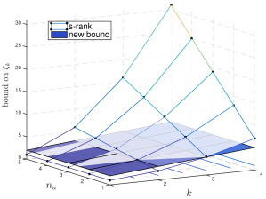
Figure 1: Bound on Helly’s dimension using the s-rank and new bound (Proposition 3) for $k\in\{1,\ldots,4\}$ and $n_{u}\in\{1,\ldots,5\}$.

5.2.2 Empirical Confidence and Violation Probability

For $n_{u}=5$ and $T=15$, Figure 2 depicts empirical estimates of the confidence $\hat{\beta}_{k}$ along the stages for both the s-rank and the new bound, while Figure 3 shows the empirical violation probability $\hat{\epsilon}_{k}$. Note that, for reasons of computational tractability, different values $\epsilon$ and $\beta$ were used in the two figures. The sample sizes $N_{k}$ used to generate both plots were acquired by numerically inverting (3) with $\zeta_{k}^{\text{new}}$ and $\zeta_{k}^{\text{s-r}}$ in place of $\zeta$, respectively.

Figures 2 and 3 show that the new bound is closer to the predefined confidence and violation probability levels (red) than the s-rank whenever $k\geq 2$, but that the s-rank outperforms the new bound only for $k=1$. This is not surprising, since for $k=1$, the s-rank provides a tighter bound on $\zeta_{1}$ than the new bound does, see also Figure 1 and Table 1. From these figures we conclude that for most stages, the new bound is less conservative than the s-rank, and therefore also the standard bound.

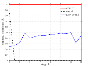
Figure 2: Predefined $\beta$ (red), its empirical estimate using the s-rank (black) and the new bound (blue) for $n_{u}=5$, $\epsilon=0.2$ and $\beta=0.1$. The estimates are obtained from $10^{4}$ instances, where for each instance the empirical violation probabilities are estimated by evaluating the solutions of each RMPC problem against $10^{4}$ uncertainty realizations. Then, $\hat{\beta}$ is determined as the fraction $\hat{\epsilon}$ which were higher than the predetermined level of $\epsilon=0.2$.

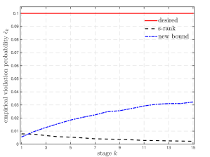
Figure 3: Predefined $\epsilon$ (red), its empirical estimate using the s-rank (black) and the new bound (blue) for $n_{u}=5$, $\epsilon=0.1$ and $\beta=10^{-7}$. The estimates are obtained by averaging over the empirical violation probabilities of $10^{3}$ instances, each estimated by evaluating its solution against $10^{4}$ uncertainty realizations.

5.2.3 Tightness of the Bounds

Even if the new bound improves upon the existing ones, Figures 2 and 3 suggest they are still conservative. Indeed, the empirical violation probabilities $\hat{\epsilon}_{k}$ can be improved using a so-called sampling-and-discarding method, in which a larger number of samples is drawn, but some of them are discarded a posteriori [31, 12]. In general, this method not only improves the objective value, but also brings the empirical violation probability closer to the predefined level. Furthermore, we can improve the empirical confidence $\hat{\beta}_{k}$ using the bound $\tilde{\zeta}_{k}^{\text{new}}=k$ instead of $\zeta_{k}^{\text{new}}=k+1$ from [18, Proposition 2], since both assumptions required there (absolutely continuous distribution and $G(x^{\star})\neq 0$) are satisfied here.

6 Conclusion

We presented a new upper bound on Helly’s dimension for random convex programs in which the constraint functions can be separated between the decision and uncertainty variables. As a consequence, the number of scenarios can be reduced significantly for problems where the dimension of the uncertain variable is smaller than the dimension of the decision variable. This leads to less conservative solutions, both in terms of cost and violation probability, as well as a reduction in the computational complexity of solutions based on the scenario approach. We applied our bounds to Stochastic MPC problems for chance constrained systems, and demonstrated the quality of the bound on an inventory example. We believe that both theoretical and applied research in the field of Randomized MPC for uncertain linear systems can benefit from our results.

Appendix A Proofs

For ease of presentation we first show the proof of Proposition 1 and then the proof of Lemma 1.

Proof of Proposition 1

Let us first prove the following auxiliary statement.

Claim.

If $r=1$, then $|\textnormal{sc}(\textnormal{SP}[\omega])|\leq m$.

Proof.

Consider $\text{SP}[\omega]$ subject to $N\geq m+1$ sampled constraints, generated by $\omega=\{\delta^{(1)},\ldots,\delta^{(N)}\}$. Suppose, for the sake of contradiction, that there exists $m+1$ support constraints. Without loss of generality, they are generated by the first $m+1$ samples, i.e. $\text{sc}(\text{SP}[\omega])=\{\delta^{(1)},\ldots,\delta^{(m+1)}\}$. Let $x^{\star}$ be the optimal solution of $\text{SP}[\omega]$ and $x_{i}^{\star}$ be the optimal solution of $\text{SP}[\omega\setminus\{\delta^{(i)}\}]$, so that $c^{\top}x^{\star}_{i}<c^{\top}x^{\star}$. If we define $p_{0}:=G(x^{\star}),\ p_{1}:=G(x^{\star}_{1}),\ \ldots,\ p_{m+1}:=G(x^{\star}_{m+1})$, then $\mathcal{P}:=\big{\{}p_{0},p_{1},p_{2},\ldots,p_{m+1}\big{\}}$ is a collection of $m+2$ vectors in $\mathbb{R}^{m}$. By Radon’s Theorem, there exist two index sets $K,L\subseteq\{0,\ldots,m+1\},\ K\cup L=\{0,\ldots,m+1\},\ K\cap L=\varnothing$, such that $\mathcal{P}$ can be partitioned into two disjoint sets $\mathcal{P}_{K}:=\{p_{k}\mid k\in K\}$ and $\mathcal{P}_{L}:=\{p_{l}\mid l\in L\}$, with $\text{conv}(\mathcal{P}_{K})\cap\text{conv}(\mathcal{P}_{L})\neq\varnothing$. Therefore there exists $\bar{p}\in\text{conv}(\mathcal{P}_{K})\cap\text{conv}(\mathcal{P}_{L})\subseteq\mathbb{R}^{m}$. Because $\bar{p}\in\text{conv}(\mathcal{P}_{K})$, there exist non-negative scalars $\{\bar{\kappa}_{k}\}_{k\in K}$, $\sum_{k\in K}\bar{\kappa}_{k}=1$, such that $\bar{p}=\sum_{k\in K}\bar{\kappa}_{k}p_{k}$. Moreover, for all $k\in K$ it holds that $p_{k}^{\top}q(\delta^{(l)})+s(\delta^{(l)})\leq 0$ $\forall l\in L\setminus\{0\}$. Therefore, since $\bar{p}\in\text{conv}(\mathcal{P}_{K})$ and $\sum_{k\in K}\bar{\kappa}_{k}=1$, it holds $\bar{p}^{\top}q(\delta^{(l)})+s(\delta^{(l)})\leq 0$ $\forall l\in L\setminus\{0\}$. Since $\bar{p}$ also belongs to $\text{conv}(\mathcal{P}_{L})$, we can analogously conclude that $\bar{p}^{\top}q(\delta^{(k)})+s(\delta^{(k)})\leq 0$ $\forall k\in K\setminus\{0\}$. Hence, since $K\cup L\supseteq\{1,\ldots,m+1\}$, it holds that $\bar{p}^{\top}q(\delta^{(i)})+s(\delta^{(i)})\leq 0$ $\forall i\in\{1,\ldots,m+1\}$. Without loss of generality, we now assume that $0\not\in K$, i.e. $G(x^{\star})\not\in\mathcal{P}_{K}$ and let $\bar{x}:=\sum_{k\in K}\bar{\kappa}_{k}x_{k}^{\star}$.

From the convexity of $g(\cdot,\delta)$, for every $i\in\{1,\ldots,N\}$ it holds that $g(\bar{x},\delta^{(i)})\leq\sum_{k\in K}\bar{\kappa}_{k}g(x^{\star}_{k},\delta^{(i)})=\sum_{k\in K}\bar{\kappa}_{k}\left[p_{k}^{\top}q(\delta^{(i)})+s(\delta^{(i)})\right]=\bar{p}^{\top}q(\delta^{(i)})+s(\delta^{(i)})\leq 0$, i.e., $\bar{x}$ is a feasible point of $\text{SP}[\omega]$. Since $c^{\top}x_{i}^{\star}<c^{\top}x^{\star}$ $\forall i\in\{1,\ldots,m+1\}$, we have $c^{\top}\bar{x}<c^{\top}x^{\star}$. This, however, contradicts the fact that $x^{\star}$ is the optimizer of $\text{SP}[\omega]$. ∎

Let now $r\geq 1$. From the above claim it holds that the number of support constraint for each row is at most $m$. Therefore, with $rm$ constraints, there are at most $rm$ support constraints. This concludes the proof. ∎

Proof of Lemma 1

The constraint $G(x)\,q(\delta)+H(x)+s(\delta)\leq 0$ can be expressed as $g(x,\delta)=\tilde{G}(x)\,\tilde{q}(\delta)+s(\delta)\leq 0$ by choosing $\tilde{G}(x):=[G(x)\ H(x)]$ and $\tilde{q}(\delta):=[q(\delta);\mathbf{1}]\in\mathbb{R}^{m+1}$. Invoking Proposition 1, we immediately get at most $r(m+1)$ support constraints. ∎

Proof of Proposition 4

We proceed in two steps and first prove the statement.

Claim.

If $r=1$, then $|\textnormal{sc}(\textsc{SP}[\omega])|\leq d(d+3)/2+1$.

Proof.

The term $\delta^{\top}A(x)\delta$ can be equivalently written as ${p}_{1}(x)^{\top}{q}_{1}(\delta)$ for some properly defined ${p}_{1}(x)$ and ${q}_{1}(\delta)$. Indeed, if $\delta_{i}$ is the $i$th component of $\delta$, then ${q}_{1}(\delta)$ contains the auxiliary uncertainties $\delta_{i}\delta_{j}$ for $i,j=1,\ldots,d$. Because $\delta_{i}\delta_{j}=\delta_{j}\delta_{i}$, it follows from symmetry that ${q}_{1}(\delta)\in\mathbb{R}^{d(d+1)/2}$. As in the affine case, the remaining term $b(x)^{\top}\delta+c(x)$ can be decomposed as ${p}_{2}(x)^{\top}{q}_{2}(\delta)$ with $p_{2}(x)^{\top}:=[b^{\top}(x)\ c(x)]$ and $q_{2}(\delta)=[\delta;1]\in\mathbb{R}^{d+1}$. Hence, the constraint can be written as $g(x,\delta)=p(x)^{\top}q(\delta)$, where $p(x):=[p_{1}(x);p_{2}(x)]$ and $q(\delta):=[q_{1}(\delta);q_{2}(\delta)]\in\mathbb{R}^{d(d+3)/2+1}$. The claim then follows from Proposition 1 with $m=d(d+3)/2+1$ and $s(\delta)=0$. ∎

We now let $r\geq 1$. Since each constraint $g_{i}$ has at most $d(d+3)/2+1$ support constraints, with $r$ constraints there are at most $rd(d+3)/2+r$ support constraints.∎

Proof of Proposition 5

We proceed similar as in the proof of Proposition 1.

Claim.

If $r=1$, then $|\textnormal{sc}(\textnormal{SP}[\omega])|\leq m$.

Proof (Sketch)..

The first part is identical to the first paragraph of the proof of the claim in Proposition 1 with the difference that $\bar{p}=\sum_{k\in K}\bar{\kappa}_{k}p_{k}$ satisfies $\underline{g}\leq\bar{p}^{\top}q(\delta^{(i)})+s(\delta^{(i)})\leq\bar{g}\ \forall i\in\{1,\ldots,m+1\}$. Moreover, by affinity of $g_{\textnormal{mult}}(\cdot,\delta)$ it follows $g_{\textnormal{mult}}(\bar{x},\delta^{(i)})=\sum_{k\in K}\bar{\kappa}_{k}g_{\textnormal{mult}}(x^{\star}_{k},\delta^{(i)})=\bar{p}^{\top}q(\delta^{(i)})+s(\delta^{(i)})$, so that for every $i\in\{1,\ldots,N\}$ we have $\underline{g}\leq g_{\textnormal{mult}}(\bar{x},\delta^{(i)})\leq\overline{g}$, i.e. $\bar{x}$ is a feasible point of SP$[\omega]$ with cost $c^{\top}\bar{x}<c^{\top}x^{\star}$. This, however, contradicts the fact that $x^{\star}$ is the optimizer of SP$[\omega]$. ∎

The proposition follows immediately since $r$ such constraints can generate at most $rm$ support constraints. ∎

References

- [1] C.E. Garcia, D.M. Prett, and M. Morari. Model predictive control: theory and practice - a survey. Automatica, 25:335–348, 1989.
- [2] J. Maciejowski. Predictive control: with constraints. Prentice Hall, 2002.
- [3] S. Boyd, L. El Ghaoui, E. Feron, and V. Balakrishnan. Linear matrix inequalities in systems and control theory, volume 15. Society for Industrial and Applied Mathematics (SIAM), 1994.
- [4] R. Tempo, G. Calafiore, and F. Dabbene. Randomized algorithms for analysis and control of uncertain systems. Springer-Verlag, 2013.
- [5] D. Mayne. Model predictive control: Recent developments and future promise. Automatica, 50(12):2967 – 2986, 2014.
- [6] A. Ben-Tal and A. Nemirovski. Robust convex optimization. Mathematics of Operations Research, 23(4):769–805, 1998.
- [7] A. Prékopa. Stochastic Programming. Mathematics and Its Applications. Springer Verlag, 1995.
- [8] M. Anthony and N. Biggs. Computational Learning Theory. Cambridge Tracts in Theoretical Computer Science, 1992.
- [9] M. Vidyasagar. Randomized algorithms for robust controller synthesis using statistical learning theory. Automatica, 37:1515–1528, 2001.
- [10] G. Calafiore and M. C. Campi. Uncertain convex programs: randomized solutions and confidence levels. Mathematical Programming, 102(1):25–46, 2005.
- [11] M. C. Campi and S. Garatti. The exact feasibility of randomized solutions of robust convex programs. SIAM Journal on Optimization, 19(3):1211–1230, 2008.
- [12] G. C. Calafiore. Random convex programs. SIAM Journal on Optimization, 20(6):3427–3464, 2010.
- [13] G. Calafiore and M. C. Campi. The scenario approach to robust control design. IEEE Trans. on Automatic Control, 51(5):742–753, 2006.
- [14] X. Zhang, G. Schildbach, D. Sturzenegger, and M. Morari. Scenario-based MPC for Energy-Efficient Building Climate Control under Weather and Occupancy Uncertainty. In Proc. of the European Control Conference, Zurich, Switzerland, 2013.
- [15] A. Parisio, D. Varagnolo, Marco Molinari, G. Pattarello, Luca Fabietti, and K. H. Johansson. Implementation of a scenario-based MPC for HVAC systems: an experimental case study. In IFAC World Congress, Cape Town, South Africa, 2014.
- [16] X. Zhang, E. Vrettos, M. Kamgarpour, and G. Andersson.and J. Lygeros. Stochastic frequency reserve provision by chance-constrained control of commercial buildings. In Proc. of European Control Conference, Linz, Austria, 2015.
- [17] G. Schildbach, L. Fagiano, and M. Morari. Randomized solutions to convex programs with multiple chance constraints. SIAM Journal on Optimization, 23(4):2479–2501, 2013.
- [18] X. Zhang, S. Grammatico, G. Schildbach, P. Goulart, and J. Lygeros. On the sample size of randomized MPC for chance-constrained systems with application to building climate control. In Proc. of the European Control Conference, Strasbourg, France, 2014.
- [19] S. Grammatico, X. Zhang, K. Margellos, P. Goulart, and J. Lygeros. A scenario approach for non-convex control design. IEEE Trans. on Automatic Control. Available online at: dx.doi.org/10.1109/TAC.2015.2433591, 2016.
- [20] P. Mohajerin Esfahani, T. Sutter, and J. Lygeros. Performance bounds for the scenario approach and an extension to a class of non-convex programs. IEEE Trans. on Automatic Control, 60(1):46–58, 2015.
- [21] S. Grammatico, X. Zhang, K. Margellos, P. Goulart, and J. Lygeros. A scenario approach to non-convex control design: preliminary probabilistic guarantees. In IEEE American Control Conference, Portland, Oregon, USA, 2014.
- [22] G. C. Calafiore, D. Lyons, and L. Fagiano. On mixed-integer random convex programs. In Proc. of the IEEE Conf. on Decision and Control, pages 3508–3513, Maui, Hawai’i, USA, 2012.
- [23] X. Zhang, S. Grammatico, K. Margellos, P. Goulart, and J. Lygeros. Randomized Nonlinear MPC for Uncertain Control-Affine Systems with Bounded Closed-Loop Constraint Violations. In IFAC World Congress, Cape Town, South Africa, 2014.
- [24] K. Margellos, P. Goulart, and J. Lygeros. On the road between robust optimization and the scenario approach for chance constrained optimization problems. IEEE Transactions on Automatic Control, 59(8):2258–2263, Aug 2014.
- [25] X. Zhang, K. Margellos, P. Goulart, and J. Lygeros. Stochastic Model Predictive Control Using a Combination of Randomized and Robust Optimization. In Proc. of the IEEE Conf. on Decision and Control, Florence, Italy, 2013.
- [26] X. Zhang, A. Georghiou, and J. Lygeros. Convex Approximation of Chance-Constrained MPC through Piecewise Affine Policies using Randomized and Robust Optimization. In Proc. of the IEEE Conf. on Decision and Control, Osaka, Japan, 2015.
- [27] G. Calafiore and L. Fagiano. Robust model predictive control via scenario optimization. IEEE Trans. on Automatic Control, 58(1):219–224, 2013.
- [28] G. Schildbach, L. Fagiano, C. Frei, and M. Morari. The scenario approach for Stochastic Model Predictive Control with bounds on closed-loop constraint violations. Automatica, 50(12):3009 – 3018, 2014.
- [29] A. Ben-Tal, A. Goryashko, E. Guslitzer, and A. Nemirovski. Adjustable robust solutions of uncertain linear programs. Mathematical Programming, 99(2):351–376, 2004.
- [30] P.J. Goulart, E.C. Kerrigan, and J.M. Maciejowski. Optimization over state feedback policies for robust control with constraints. Automatica, 42(4):523–533, 2006.
- [31] M. C. Campi and S. Garatti. A sampling-and-discarding approach to chance-constrained optimization: feasibility and optimality. Journal of Optimization Theory and Applications, 148(2):257–280, 2011.