Factors controlling the time-delay between peak CO₂ emissions and concentrations

Abstract

Carbon-dioxide (CO₂) is the main contributor to anthropogenic global warming, and the timing of its peak concentration in the atmosphere is likely to govern the timing of maximum radiative forcing. It is well-known that dynamics of atmospheric CO₂ is governed by multiple time-constants, and here we approximate the solutions to a linear model of atmospheric CO₂ dynamics with four time-constants to identify factors governing the time-delay between peaks in CO₂ emissions and concentrations, and therefore the timing of the concentration peak. The main factor affecting this time-delay is the ratio of the rate of change of emissions during its increasing and decreasing phases. If this ratio is large in magnitude then the time-delay between peak emissions and concentrations is large. Therefore it is important to limit the magnitude of this ratio through mitigation, in order to achieve an early peak in CO₂ concentrations. This can be achieved with an early global emissions peak, combined with rapid decarbonization of economic activity, because the delay between peak emissions and concentrations is affected by the time-scale with which decarbonization occurs. Of course, for limiting the magnitude of peak concentrations it is also important to limit the magnitude of emissions throughout its trajectory, but that aspect has been studied elsewhere and is not examined here. The carbon cycle parameters affecting the timing of the concentration peak are primarily the long multi-century time-constant of atmospheric CO₂, and the ratio of contributions to the impulse response function of atmospheric CO₂ from the infinite time-constant and the long time-constant respectively. Reducing uncertainties in these parameters can reduce uncertainty in forecasts of the radiative forcing peak.

Divecha Centre for Climate Change, Indian Institute of Science, Bangalore 560012. India. (ashwin@fastmail.fm)

Keywords

Global climate change; carbon dioxide; peak radiative forcing; climate change mitigation; decarbonization.

1 Introduction

As countries agree on commitments towards a new international climate treaty to be decided in 2015 (UNFCCC (2014a, b)), these will include mitigation of not only carbon-dioxide (CO₂) but also other climate forcers (UNFCCC (2014c)). CO₂ is, and is likely to remain, the largest contribution to radiative forcing (Forster et al. (2007); Myhre et al. (2013)). Limiting long-term warming requires limiting the growth in global CO₂ emissions, and eventually reducing these emissions. If the present increasing trend in global CO₂ emissions is eventually reversed so that an emissions peak occurs, the corresponding peak in concentration will be delayed because of its long atmospheric lifetime (Allen et al. (2009); Meinshausen et al. (2009); Mignone et al. (2008)). A CO₂ concentration peak would be a significant event for global climate: it would govern the maximum contribution of CO₂ emissions to radiative forcing. Furthermore, assuming that CO₂ continues to be the major contribution to radiative forcing, then its peak concentration will strongly influence the magnitude and timing of peak global warming.

The Earth’s CO₂ cycle is complex, involving multiple reservoirs that maintain exchanges occurring at very different rates (Archer et al. (1997); Cox et al. (2000); Falkowski et al. (2000)). The most rapid uptake of excess CO₂ is by the surface ocean and land biosphere (Pierrehumbert (2014)). Progressively slower processes involve mixing with the deep-ocean, reduction of ocean acidity due to dissolution of carbonates, and uptake of excess atmospheric CO₂ via reaction with CaCO₃ or silicate rocks on land (Archer et al. (1997); Archer and Brovkin (2008); Archer et al. (2009)). The last two processes require many tens of thousands of years so that, on the timescales of the next few centuries, their contributions can be effectively neglected. Equivalently their effects can be treated as occurring with infinite time-constant. Accurate characterization of the different processes involved, in order to describe the fate of excess atmospheric CO₂, requires coupled climate-carbon-cycle or Earth-system models; such models have been employed to describe effects of mitigation scenarios on CO₂ in the atmosphere (Petoukhov et al. (2005); Friedlingstein et al. (2006)). As the mitigation of CO₂ emissions unfolds, these and similar models will play important roles in estimating the consequences for atmospheric CO₂, including the timing and magnitude of its peak concentration.

This paper solves a linear model of atmospheric CO₂ with four time-constants (Joos et al. (2013)) to understand the factors controlling the time-delay between peaks in emission and concentration and therefore the timing of the concentration peak. Previous studies have described the relationship between mitigation and warming, and highlighted the importance of rapid mitigation (for e.g. Socolow and Lam (2007); Allen et al. (2009); Allen and Stocker (2014); Huntingford et al. (2012)). Here we focus specifically on solving the model of atmospheric CO₂ analytically, to identify some of the important factors controlling the time to the concentration peak of CO₂.

2 Models of emissions and carbon cycle

2.1 Carbon cycle model

Joos et al. (2013) estimated the impulse response of CO₂ in the Earth’s atmosphere, by averaging a group of Earth System Models. They estimated a mean response with four time-constants

$$h\left(t\right)=0.276e^{-t/4.30}+0.282e^{-t/36.5}+0.224e^{-t/394}+0.217$$ (1)

which we apply, and compute atmospheric concentration using

$$u\left(t\right)=\int_{0}^{t}m\left(z\right)h\left(t-z\right)dz+u_{P}$$ (2)

where $m\left(z\right)$ is anthropogenic emissions in concentration units, i.e. the rate of increase in concentration in the hypothetical case of infinite atmospheric lifetime. The constant term $u_{P}$ is preindustrial concentration. Concentration is noted in parts per million (ppm). Atmospheric emission of CO₂ in the year 2013 was $36\times 10^{12}$ kg, equivalent to $4.5$ ppm. We furthermore describe the impulse response function symbolically as

$$h\left(t\right)=\sum_{i=1}^{K}\mu_{i}e^{-t/\tau_{i}}$$ (3)

with $\sum_{i=1}^{K}\mu_{i}=1$ and $\left\{\tau_{1},\tau_{2},\tau_{3},\tau_{4}\right\}=\left\{4.4,36.5,394,\infty\right\}$ following the results of Joos et al. (2013). The infinite time-constant approximates the effects of very slow processes involving buffering of ocean acidity by dissolution of carbonates and the uptake of CO₂ in the weathering of rocks.

There is uncertainty in the function $h\left(t\right)$, with different earth system models likely to yield different results (Joos et al. (2013)). While the present paper does not characterize this uncertainty, Section 3.3 considers the influence of changing those parameters in this 4-time-constant model that are shown to affect the timing of the concentration peak.

2.2 Emissions model

The model of emissions $m\left(t\right)$ is very simple, and chosen so as to describe emissions using a few different parameters that can be readily interpreted. The emissions model is $m\left(t\right)=m_{0}\left(1+r\right)^{\left(min\left(t,t_{g}\right)-t_{0}\right)}e^{-\left(t-t_{0}\right)/\tau_{m}}$ (Seshadri (2015a, b)), with $m_{0}$ being present emissions, $r$ the growth rate of gross global product (GGP), and $t_{0}$ denoting the present time. It is assumed, for the purposes of the emissions model used here, that GGP increases for $t_{g}$ years from the present at constant rate $r$, after which it remains fixed. The term $e^{-\left(t-t_{0}\right)/\tau_{m}}$ describes the effect of decrease in emissions intensity of economic output, with $\tau_{m}\rightarrow\infty$ corresponding to the absence of any mitigation, and smaller values of $\tau_{m}$ corresponding to rapid mitigation. This model of emissions has been borrowed from previous work (Seshadri (2015a, b)).

3 Results

3.1 Peak atmospheric concentration of CO2

With emissions $m\left(t\right)$ the atmospheric concentration is $u\left(t\right)=u_{P}+\int_{0}^{t}m\left(z\right)h\left(t-z\right)dz$, and differentiating this equation we obtain for the rate of change of concentration that $u^{\prime}\left(t\right)=m\left(t\right)+\int_{0}^{t}m\left(z\right)\frac{\partial h\left(t-z\right)}{\partial t}dz$, where we have used the fact that $h\left(0\right)=1$ from equation (1). Using equation (3) we obtain that $u^{\prime}\left(t\right)=m\left(t\right)-\sum_{i=1}^{K}\frac{\mu_{i}}{\tau_{i}}e^{-t/\tau_{i}}\int_{0}^{t}e^{z/\tau_{i}}m\left(z\right)dz$. The last integral can be evaluated by parts to give $\int_{0}^{t}e^{z/\tau_{i}}m\left(z\right)dz=\tau_{i}m\left(t\right)e^{t/\tau_{i}}-\tau_{i}\int_{0}^{t}e^{z/\tau_{i}}m^{\prime}\left(z\right)dz$, and substituting this yields

$$u^{\prime}\left(t\right)=\sum_{i=1}^{K}\mu_{i}e^{-t/\tau_{i}}\int_{0}^{t}e^{z/\tau_{i}}m^{\prime}\left(z\right)dz$$ (4)

for the rate of change of concentration. This result has been derived previously in Seshadri (2015c).

For short time-constants $\tau_{1}=4.4$ years and $\tau_{2}=36.5$ years for which $t\gg\tau_{i}$, $i=1,2$, we can approximate the integral $\int_{0}^{t}e^{z/\tau_{i}}m^{\prime}\left(z\right)dz$ by $\tau_{i}e^{t/\tau_{i}}m^{\prime}\left(t\right)$ . For the very long time-constant that is represented by $\tau_{4}=\infty$ the integral becomes $\int_{0}^{t}e^{z/\tau_{i}}m^{\prime}\left(z\right)dz=\int_{0}^{t}m^{\prime}\left(z\right)dz=m\left(t\right)$ . Hence the rate of change of concentration becomes approximately

$$u^{\prime}\left(t\right)\cong\left(\mu_{1}\tau_{1}+\mu_{2}\tau_{2}\right)m^{\prime}\left(t\right)+\mu_{3}e^{-t/\tau_{3}}\int_{0}^{t}e^{z/\tau_{3}}m^{\prime}\left(z\right)dz+\mu_{4}m\left(t\right)$$ (5)

We denote the time to the emissions peak as $t_{1}$, the time to the concentration peak as $t_{2}$, and the time-delay as $\delta t\equiv t_{2}-t_{1}$. Then the integral in equation (5) above can be described as the sum of integrals from $0$ to $t_{1}$, and from $t_{1}$ to $t_{2}$. Furthermore, defining weighted rates of change of emissions

$$m^{\prime}_{av,i}=\frac{\int_{0}^{t_{1}}e^{z/\tau_{3}}m^{\prime}\left(z\right)dz}{\int_{0}^{t_{1}}e^{z/\tau_{3}}dz}$$ (6)

and

$$m^{\prime}_{av,d}=\frac{\int_{t_{1}}^{t_{2}}e^{z/\tau_{3}}m^{\prime}\left(z\right)dz}{\int_{t_{1}}^{t_{2}}e^{z/\tau_{3}}dz}$$ (7)

we obtain the formula for the rate of change of concentration at time $t=t_{2}$

$$u^{\prime}\left(t_{2}\right)\cong\left(\mu_{1}\tau_{1}+\mu_{2}\tau_{2}\right)m^{\prime}\left(t_{2}\right)+\mu_{3}\tau_{3}m^{\prime}_{av,i}e^{-t_{2}/\tau_{3}}\left(e^{t_{1}/\tau_{3}}-1\right)+\mu_{3}\tau_{3}m^{\prime}_{av,d}e^{-t_{2}/\tau_{3}}\left(e^{t_{2}/\tau_{3}}-e^{t_{1}/\tau_{3}}\right)+\mu_{4}m\left(t_{2}\right)$$ (8)

Before proceeding we identify the factors influencing whether the concentration will reach a peak value and eventually decline, as opposed to continuing to increase to an asymptotic maximum. Consider emissions scenarios where the emissions peaks and then declines to zero so that, eventually, $m^{\prime}\left(t\right)=0$ and $m\left(t\right)=0$. In that case only the large but finite time-constant $\tau_{3}=394$ years in the model of Joos et al. (2013) plays a role in the sign of $u^{\prime}\left(t\right)$. The value of this quantity then becomes, for $t>t_{1}$, approximately

$$u^{\prime}\left(t\right)\cong\mu_{3}\tau_{3}m^{\prime}_{av,i}e^{-t/\tau_{3}}\left(e^{t_{1}/\tau_{3}}-1\right)+\mu_{3}\tau_{3}m^{\prime}_{av,d}e^{-t/\tau_{3}}\left(e^{t/\tau_{3}}-e^{t_{1}/\tau_{3}}\right)$$ (9)

which is negative if

$$-m^{\prime}_{av,d}>m^{\prime}_{av,i}\frac{e^{t_{1}/\tau_{3}}-1}{e^{t/\tau_{3}}-e^{t_{1}/\tau_{3}}}$$ (10)

requiring the rate of decrease of emissions to be sufficiently large in magnitude. The larger the average rate of increase in emissions, and the longer the increase persists, the more stringent is the condition on the subsequent decrease in order for concentrations to eventually decrease. Therefore an early peak in global emissions can help stabilize atmospheric CO₂ concentrations, as would be expected.

We now seek an expression for the time $t_{2}$ to the CO₂ concentration peak, assuming that mitigation occurs rapidly enough for one to occur. The condition for such a peak is that the rate of change of concentration vanishes. Hence, from equation (8) above

$$u^{\prime}\left(t_{2}\right)\cong\left(\mu_{1}\tau_{1}+\mu_{2}\tau_{2}\right)m^{\prime}\left(t_{2}\right)+\mu_{3}\tau_{3}m^{\prime}_{av,i}e^{-t_{2}/\tau_{3}}\left(e^{t_{1}/\tau_{3}}-1\right)+\mu_{3}\tau_{3}m^{\prime}_{av,d}e^{-t_{2}/\tau_{3}}\left(e^{t_{2}/\tau_{3}}-e^{t_{1}/\tau_{3}}\right)+\mu_{4}m\left(t_{2}\right)=0$$ (11)

and, writing $m\left(t_{2}\right)=m^{\prime}_{i}t_{1}+m^{\prime}_{d}\left(t_{2}-t_{1}\right)$, where $m^{\prime}_{i}$ and $m^{\prime}_{d}$ are average rates of change during emission’s increasing and decreasing phases respectively, and collecting terms involving $t_{2}$ yields

$$\mu_{3}\tau_{3}e^{-t_{2}/\tau_{3}}\left(\left(m^{\prime}_{av,i}-m^{\prime}_{av,d}\right)e^{t_{1}/\tau_{3}}-m^{\prime}_{av,i}\right)+\mu_{4}m^{\prime}_{d}t_{2}\cong-\mu_{3}\tau_{3}m^{\prime}_{av,d}-\mu_{4}\left(m^{\prime}_{i}-m^{\prime}_{d}\right)t_{1}-\left(\mu_{1}\tau_{1}+\mu_{2}\tau_{2}\right)m^{\prime}\left(t_{2}\right)$$ (12)

We can neglect the last term on the right side of equation (12), since $m^{\prime}\left(t_{2}\right)$ is comparable in magnitude to $m^{\prime}_{av,d}$, as will be shown, but $\mu_{1}\tau_{1}+\mu_{2}\tau_{2}\ll\mu_{3}\tau_{3}$. Hence the time $t_{2}$ to the concentration peak in the model is governed by approximate equality

$$\mu_{3}\tau_{3}e^{-t_{2}/\tau_{3}}\left(m^{\prime}_{av,i}-\left(m^{\prime}_{av,i}-m^{\prime}_{av,d}\right)e^{t_{1}/\tau_{3}}\right)-\mu_{4}m^{\prime}_{d}t_{2}\cong\mu_{3}\tau_{3}m^{\prime}_{av,d}+\mu_{4}\left(m^{\prime}_{i}-m^{\prime}_{d}\right)t_{1}$$ (13)

The approximate equality in equation (13) has been verified in Figure 1c, for emissions scenarios shown in Figure 1a and corresponding concentration graphs plotted in Figure 1b. It is therefore confirmed that the short time-constants can be approximately neglected while studying the concentration peak. The above equation has to be solved numerically because neither the exponential nor the linear term in $t_{2}$ on the left side of the expression can be neglected. That this is the case is shown in Figure 1d, which plots these two terms. Neither term is dominant.

However in order to understand qualitatively the factors influencing the time $t_{2}$, let us imagine that $t_{2}$ is so large that the second term in the left side of equation (13), $-\mu_{4}m^{\prime}_{d}t_{2}$, were dominant. Then the solution would be given by

$$t_{2}\cong\tau_{3}\left(\left(\frac{m^{\prime}_{i}}{-m^{\prime}_{d}}+1\right)\frac{t_{1}}{\tau_{3}}+\frac{\mu_{3}}{\mu_{4}}\frac{m^{\prime}_{av,d}}{-m^{\prime}_{d}}\right)$$ (14)

The time to the concentration peak increases with the rate of increase of emissions during their growing phase. It decreases with the rate of decrease of emissions during their declining phase. The time to the concentration peak increases with the ratio $\mu_{4}/\mu_{3}$, describing the ratio of the impulse response of atmospheric CO₂ coming from the infinite time-constant $\tau_{4}$ and finite but long time-constant $\tau_{3}$ respectively. It increases with the time $t_{1}$ to the emissions peak, and in fact the influence of $t_{1}$ can be described in terms of dimensionless ratio $t_{1}/\tau_{3}$. However the left side of equation (13) increases with $t_{1}$, because of the exponential term, so the influence of $t_{1}$ is not as strong as equation (14), which neglects the influence of this term, would suggest. Similarly the influence of $\tau_{3}$ is not as strong as equation (14) would suggest because the exponential term in equation (13) also increases with this quantity.

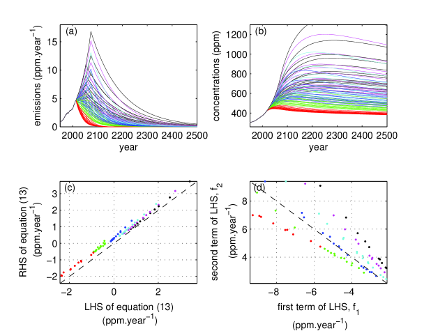
Figure 1: Verification of approximation in equation (13) and demonstration that neither term on the left side of this equation is dominant for a wide range of CO₂ emissions scenarios: (a) emissions pathways; (b) corresponding graphs of CO₂ concentration; (c) each side of equation (13), with left side in abscissa and right side in ordinate. The dashed line shows where abscissa and ordinate are equal; (d) first and second terms on the left side of equation (13), $f_{1}=\mu_{3}\tau_{3}e^{-t_{2}/\tau_{3}}\left(m^{\prime}_{av,i}-\left(m^{\prime}_{av,i}-m^{\prime}_{av,d}\right)e^{t_{1}/\tau_{3}}\right)$ and $f_{2}=-\mu_{4}m^{\prime}_{d}t_{2}$ , showing that neither term is dominant. Dashed line shows were abscissa and ordinate are of equal magnitude. Colors in panels correspond to different e-folding mitigation timescales in the respective emissions scenarios (see legend in Figure 2).

We can write equation (13) in terms of dimensionless variables $m^{\prime}_{av,i}/m^{\prime}_{av,d}$, $t_{1}/\tau_{3}$, and parameter $\mu_{4}/\mu_{3}$, by writing it in equivalent form

$$\tau_{3}e^{-t_{2}/\tau_{3}}\left(\frac{m^{\prime}_{av,i}}{m^{\prime}_{av,d}}-\left(\frac{m^{\prime}_{av,i}}{m^{\prime}_{av,d}}-1\right)e^{t_{1}/\tau_{3}}\right)-\frac{\mu_{4}}{\mu_{3}}\frac{m^{\prime}_{d}}{m^{\prime}_{av,d}}t_{2}\cong\tau_{3}+\frac{\mu_{4}}{\mu_{3}}\left(\frac{m^{\prime}_{i}}{m^{\prime}_{av,d}}-\frac{m^{\prime}_{d}}{m^{\prime}_{av,d}}\right)t_{1}$$ (15)

The above model depends also on variables $m^{\prime}_{i}/m^{\prime}_{av,d}$ and $m^{\prime}_{d}/m^{\prime}_{av,d}$. Recall that these are ratios of unweighted rates of change and weighted rates of change, i.e. weighted by $e^{t/\tau_{3}}$. It is shown later that $m^{\prime}_{d}/m^{\prime}_{av,d}$ is approximately constant across scenarios (also see Figure 3).

Figure 2 plots the time-delay between peak emissions and concentrations versus the dimensionless variable $m^{\prime}_{av,i}/m^{\prime}_{av,d}$, for the emissions scenarios plotted in Figure 1. The time-delay increases with the absolute value of this ratio. Furthermore, for scenarios with relatively short e-folding mitigation timescale, less than about 40 years, the relationship is approximately linear for the family of scenarios considered here.

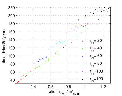
Figure 2: Time-delay $\delta t$ between peak emissions and concentrations versus the ratio of the weighted-averaged rate of increase and decrease of emissions, defined in equations (6) and (7) respectively. The time delay increases with the absolute value of this ratio. Note the reversed axis in the abscissa. For short e-folding mitigation timescales, the relationship is approximately linear. Results are shown for the scenarios in Figure 1, and colors in the plot correspond to the colors in Figures 1a-d.

3.2 Influence of mitigation parameters, and importance of e-folding mitigation timescale

Here we consider the effects of parameters of our specific emissions model on the rates $m^{\prime}_{av,i}$, $m^{\prime}_{av,d}$ , $m^{\prime}_{i}$ and $m^{\prime}_{d}$ , and thereby on the solution to equation (15). This discussion is of more general interest beyond this particular model because the parameters - the GGP growth rate, the e-folding mitigation timescale at which emissions intensity decreases, and the time to stabilization of GGP - can be easily interpreted. Considering first the rate of change of emissions during its increasing phase

$$m_{i}^{\prime}=\frac{\int_{0}^{t_{1}}m^{\prime}\left(z\right)dz}{\int_{0}^{t_{1}}dz}=\frac{m\left(t_{1}\right)}{t_{1}}$$ (16)

Approximating $\left(1+r\right)^{t}\cong e^{rt}$ the formula for emissions becomes $m\left(t_{1}\right)=m_{0}e^{r\left(t_{1}-t_{0}\right)-\left(t_{1}-t_{0}\right)/\tau_{m}}$. If $r>1/\tau_{m}$ then $t_{1}=t_{g}$, i.e. emissions peaks when GGP is maximum. Otherwise $t_{1}=t_{0},$ the present. In the first case $m\left(t_{1}\right)=m_{0}e^{\left(r-\frac{1}{\tau_{m}}\right)\left(t_{g}-t_{0}\right)}$ and $m_{i}^{\prime}=m_{0}e^{\left(r-\frac{1}{\tau_{m}}\right)\left(t_{g}-t_{0}\right)}/t_{g}$, whereas in the second case $m\left(t_{1}\right)=m_{0}$ and $m_{i}^{\prime}=m_{0}/t_{0}$.

In the following we consider only the case where $r>1/\tau_{m}$ because global emissions of CO₂ are expected to continue to increase for a while. For its decreasing phase

$$m_{d}^{\prime}=\frac{\int_{t_{1}}^{t_{2}}m^{\prime}\left(z\right)dz}{\int_{t_{1}}^{t_{2}}dz}=\frac{m\left(t_{2}\right)-m\left(t_{1}\right)}{t_{2}-t_{1}}$$ (17)

Then $m\left(t_{2}\right)=m\left(t_{1}\right)e^{-\frac{t_{2}-t_{1}}{\tau_{m}}}$ so that $m_{d}^{\prime}=-m\left(t_{1}\right)\left(1-e^{-\frac{t_{2}-t_{1}}{\tau_{m}}}\right)/\left(t_{2}-t_{1}\right)$, which becomes $-m_{0}e^{\left(r-\frac{1}{\tau_{m}}\right)\left(t_{g}-t_{0}\right)}\left(1-e^{-\frac{t_{2}-t_{g}}{\tau_{m}}}\right)/\left(t_{2}-t_{g}\right)$ .

For the weighted rate of increase of emissions between $0$ and $t_{1}$ , we decompose the integral in the numerator of equation (6) into that between $0$ and $t_{0}$ and between $t_{0}$ and $t_{1}$. Using $m^{\prime}\left(t\right)=\left(r-\frac{1}{\tau_{m}}\right)m_{0}e^{\left(r-\frac{1}{\tau_{m}}\right)\left(t-t_{0}\right)}$ between $t_{0}$ and $t_{1}$ we obtain

$$m^{\prime}_{av,i}=\frac{m^{\prime}_{av0}+m_{0}\frac{r-\frac{1}{\tau_{m}}}{r-\frac{1}{\tau_{m}}+\frac{1}{\tau_{3}}}\left(e^{\left(r-\frac{1}{\tau_{m}}\right)\left(t_{g}-t_{0}\right)+\frac{t_{g}}{\tau_{3}}}-e^{\frac{t_{0}}{\tau_{3}}}\right)}{\tau_{3}\left(e^{t_{g}/\tau_{3}}-1\right)}$$ (18)

where $m^{\prime}_{av0}=\int_{0}^{t_{0}}e^{z/\tau_{3}}m^{\prime}\left(z\right)dz$. Likewise using $m^{\prime}\left(t\right)=-\frac{m_{0}}{\tau_{m}}e^{r\left(t_{g}-t_{0}\right)-\frac{t-t_{0}}{\tau_{m}}}$ between $t_{1}$ and $t_{2}$

$$m^{\prime}_{av,d}=-\frac{m_{0}e^{\left(r-\frac{1}{\tau_{m}}\right)\left(t_{g}-t_{0}\right)}\left(e^{\frac{t_{g}}{\tau_{3}}}-e^{-\frac{t_{2}-t_{g}}{\tau_{m}}+\frac{t_{2}}{\tau_{3}}}\right)}{\left(\tau_{3}-\tau_{m}\right)\left(e^{t_{2}/\tau_{3}}-e^{t_{g}/\tau_{3}}\right)}$$ (19)

Let us compare the rates $m_{d}^{\prime}$ and $m^{\prime}_{av,d}$ by considering ratio

$$\frac{m^{\prime}_{av,d}}{m_{d}^{\prime}}=\frac{e^{\frac{t_{g}}{\tau_{3}}}\left(1-e^{-\frac{t_{2}-t_{g}}{\tau_{m}}+\frac{t_{2}-t_{g}}{\tau_{3}}}\right)}{1-e^{-\frac{t_{2}-t_{g}}{\tau_{m}}}}\frac{t_{2}-t_{g}}{\left(\tau_{3}-\tau_{m}\right)e^{\frac{t_{g}}{\tau_{3}}}\left(e^{\frac{t_{2}-t_{g}}{\tau_{3}}}-1\right)}$$ (20)

which, assuming $1/\tau_{m}\gg 1/\tau_{3}$ because the mitigation timescale is generally much shorter than this time-constant of CO₂, simplifies to

$$\frac{t_{2}-t_{g}}{\left(\tau_{3}-\tau_{m}\right)\left(e^{\frac{t_{2}-t_{g}}{\tau_{3}}}-1\right)}$$ (21)

In case $\frac{t_{2}-t_{g}}{\tau_{3}}\ll 1$ the exponential term in equation (21) simplifies to $1+\frac{t_{2}-t_{g}}{\tau_{3}}$, in which case the ratio approximates to

$$\frac{m^{\prime}_{av,d}}{m_{d}^{\prime}}\cong\frac{\tau_{3}}{\tau_{3}-\tau_{m}}$$ (22)

which, for cases where $\tau_{3}\gg\tau_{m}$, approximates to 1. Hence the value of weighted average $m^{\prime}_{av,d}$, while not exactly equal that of the average rate of change of emissions $m_{d}^{\prime}$ in its decreasing phase, closely approximates the latter, especially in cases of rapid mitigation when, in addition, the time-delay between peak emissions and concentrations is short compared to time-constant $\tau_{3}$. A near-equality between these two variables, weighted and unweighted, is seen in Figure 3b. Similarly Figure 3a shows the relationship between weighted and unweighted rates of change for the phase when emissions are increasing. While departure from equality is larger, the relationship is still approximately linear.

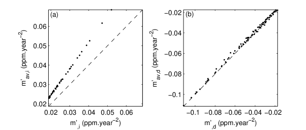
Figure 3: Plots of weighted (by $e^{t/\tau_{3}}$) versus unweighted rate of change of emissions: (a) increasing phase; (b) decreasing phase. Dashed lines show where abscissa and ordinate are equal. An approximate linear relationship holds between the two sets of variables.

Although these weighted and unweighted rates are not the same, because of their similarities we can examine ratio $m_{i}^{\prime}/m_{d}^{\prime}$ , which is more tractable, to understand qualitatively what controls the behavior of ratio $m^{\prime}_{av,i}/m^{\prime}_{av,d}$. The former ratio can be written as

$$\frac{m_{i}^{\prime}}{m_{d}^{\prime}}=-\frac{t_{2}-t_{g}}{t_{g}}\frac{1}{1-e^{-\frac{t_{2}-t_{g}}{\tau_{m}}}}$$ (23)

A longer time $t_{2}$ to the concentration peak by itself can increase the above ratio, because the graph of emissions is convex in its decreasing phase, so that its slope is decreasing. The influence of time $t_{g}$ to peak emissions is weak because of two countervailing influences: shorter $t_{g}$ increases the magnitude of the numerator as well as that of the denominator above. The main influence on this ratio is that of mitigation timescale $\tau_{m}$ . Short $\tau_{m}$ decreases the magnitude of this ratio.

The strong influence of the mitigation timescale on the ratio $m^{\prime}_{av,i}/m^{\prime}_{av,d}$ is seen in Figure 4. Short mitigation timescale, corresponding to rapid mitigation of emissions intensity, is therefore essential to limit the absolute magnitude of this ratio and therefore assure a short time-delay.

Note that the ratio in equation (23) does not depend on the GGP’s growth rate. While this rate influences peak emissions of CO₂, it affects the average growth rate and decrease of emissions in the same manner and hence is not a factor in this ratio and consequently in the time-delay between peak emissions and concentrations.

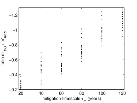
Figure 4: Ratio $m^{\prime}_{av,i}/m^{\prime}_{av,d}$ versus e-folding mitigation timescale. Note the reversed axis on the ordinate. Short mitigation timescale decreases the absolute value of this ratio.

3.3 Carbon cycle uncertainties

As indicated earlier the carbon-cycle parameters affecting the time to the concentration peak are the multi-century time-constant $\tau_{3}$ and the ratio $\mu_{4}/\mu_{3}$, describing the ratio of the impulse response of atmospheric CO₂ from the infinite time-constant $\tau_{4}$ and the long time-constant $\tau_{3}$ respectively. Figure 5 plots the influence of these parameters on the time-delay. These are the uncertainties in the carbon cycle that must be constrained in order to constrain forecasts of the timing of peak concentrations of CO₂.

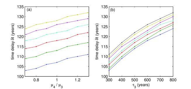
Figure 5: The main carbon cycle parameters affecting the time-delay between peak CO₂ emissions and concentrations: (a) relation between time-delay and $\mu_{4}/\mu_{3}$ describing the ratio of the impulse response of atmospheric CO₂ from the infinite time-constant $\tau_{4}$ and the long time-constant $\tau_{3}$ respectively; (b) relation between time-delay and long time-constant $\tau_{3}$. In each panel, different curves correspond to different fixed values of the other parameter. The emissions scenario used has $t_{g}-t_{0}=60$ years, $r=0.015$ %/year, and $\tau_{m}=50$ years.

4 Conclusions and Discussion

The results presented here are based on approximating the linear carbon cycle model with four time-constants of Joos et al. (2013), with one time-constant being infinite because a fraction of emitted CO₂ persists for a very long time (Archer (2005); Archer and Brovkin (2008)). We identified the main factors governing the time-delay between peak CO₂ emissions and concentrations.

On the emissions front, the main factor is the e-folding timescale with which the mitigation of emissions intensity of GGP ("decarbonization") occurs. This can be viewed as the inverse of the corresponding mitigation rate (Seshadri (2015a)). Short decarbonization timescale leads to short time-delay between emissions and concentration peaks. Therefore achieving decarbonization rapidly is important to achieving an early peak in CO₂ concentrations.

The time-delay between peak emissions and concentrations is not sensitive to the time to peak emissions. However an early emissions peak will facilitate an early concentration peak.

The growth rate of economic output is an important factor in peak emissions. However as discussed here it does not affect the time delay between peak emissions and concentrations, because it has the same effect on the rate of increase of emissions and the rate of decrease of emissions, whose ratio governs the time-delay. Therefore in this model where peak emissions corresponds to where GGP stabilizes, the timing of peak concentrations is not affected by this growth rate. Nevertheless it is obviously important in considering the magnitude of peak emissions, and faster economic growth has to be accompanied by more rapid decarbonization.

The important non-dimensional parameter in our discussion has been the ratio of the rate of increase of emissions and the rate of decrease of emissions. Limiting the magnitude of this ratio will help achieve an early peak, and this can be accomplished by keeping the mitigation timescale short.

With respect to the atmospheric cycle of CO₂, the influential parameters are the long but finite time-constant $\tau_{3}$ that occurs on century-scales, and the factor $\mu_{4}/\mu_{3}$ describing the ratio of the impulse response function of atmospheric CO₂ from the infinite time-constant $\tau_{4}$ and the long time-constant $\tau_{3}$ respectively. The time-delay increases with these parameters. The short time constants $\tau_{1}$ and $\tau_{2}$ occurring on decadal scales or less play a small role in the long-term dynamics of atmospheric CO₂, and uncertainties in their values are correspondingly less important for forecasting the concentration peak.

In summary it is important to constrain these carbon cycle parameters, in addition to achieving an early mitigation peak, as well as implementing decarbonization on short timescales.

References

- Allen and Stocker (2014) Allen, M. R., and T. F. Stocker (2014), Impact of delay in reducing carbon dioxide emissions, Nature Climate Change, 4, 23–26, doi:http://dx.doi.org/10.1038/nclimate2077.
- Allen et al. (2009) Allen, M. R., D. J. Frame, C. Huntingford, C. D. Jones, J. A. Lowe, M. Meinshausen, and N. Meinshausen (2009), Warming caused by cumulative carbon emissions towards the trillionth tonne, Nature, 458, 1163–1166, doi:http://dx.doi.org/10.1038/nature08019.
- Archer (2005) Archer, D. (2005), Fate of fossil-fuel CO2 in geologic time, Journal of Geophysical Research, 110, C09S05, doi:http://dx.doi.org/10.1029/2004JC002625.
- Archer and Brovkin (2008) Archer, D., and V. Brovkin (2008), The millennial atmospheric lifetime of anthropogenic CO2, Climatic Change, 90(3), 283–297, doi:http://dx.doi.org/10.1007/s10584-008-9413-1.
- Archer et al. (1997) Archer, D., H. Kheshgi, and E. Maier-Reimer (1997), Multiple timescales for neutralization of fossil fuel CO2, Geophysical Research Letters, 24, 405–408, doi:http://dx.doi.org/10.1029/97GL00168.
- Archer et al. (2009) Archer, D., M. Eby, V. Brovkin, A. Ridgwell, and L. Cao (2009), Atmospheric lifetime of fossil fuel carbon dioxide, Annual Review of Earth and Planetary Sciences, 37, 117–134, doi:http://dx.doi.org/10.1146/annurev.earth.031208.100206.
- Cox et al. (2000) Cox, P. M., R. A. Bett, C. D. Jones, S. A. Spall, and I. J. Totterdell (2000), Acceleration of global warming due to carbon-cycle feedbacks in a coupled climate model, Nature, 408, 184–187, doi:http://dx.doi.org/10.1038/35041539.
- Falkowski et al. (2000) Falkowski, P., R. J. Scholes, E. Boyle, J. Canadell, D. Canfield, J. Elser, N. Gruber, K. Hibbard, P. Hogberg, S. Linder, F. T. Mackenzie, B. M. III, T. Pedersen, Y. Rosenthal, S. Seitzinger, V. Smetacek, and W. Steffen (2000), The global carbon cycle: A test of our knowledge of Earth as a system, Science, 290, 291–296, doi:http://dx.doi.org/10.1126/science.290.5490.291.
- Forster et al. (2007) Forster, P., V. Ramaswamy, P. Artaxo, T. Berntsen, R. Betts, and D. Fahey (2007), Climate Change 2007: The Physical Science Basis. Contribution of Working Group I to the Fourth Assessment Report of the Intergovernmental Panel on Climate Change, chap. Changes in Atmospheric Constituents and in Radiative Forcing, Cambridge University Press.
- Friedlingstein et al. (2006) Friedlingstein, P., P. Cox, R. Betts, L. Bopp, W. von Bloh, V. Brovkin, P. Cadule, S. Doney, M. Eby, and I. Fung (2006), Climate-carbon cycle feedback analysis: Results from the C4MIP Model Intercomparison, Journal of Climate, 19, 3337–3353, doi:http://dx.doi.org/10.1175/JCLI3800.1.
- Huntingford et al. (2012) Huntingford, C., J. A. Lowe, L. K. Gohar, N. H. A. Bowerman, M. R. Allen, S. C. B. Raper, and S. M. Smith (2012), The link between a global 2C warming threshold and emissions in years 2020, 2050 and beyond, Environmental Research Letters, 7, 1–8, doi:http://dx.doi.org/10.1088/1748-9326/7/1/014039.
- Joos et al. (2013) Joos, F., R. Roth, J. S. Fuglestvedt, G. Peters, V. Brovkin, M. Eby, N. Edwards, and B. Eleanor (2013), Carbon dioxide and climate impulse response functions for the computation of greenhouse gas metrics: A multi-model analysis, Atmospheric Chemistry and Physics, 13, 2793–2825, doi:http://dx.doi.org/10.5194/acp-13-2793-2013.
- Meinshausen et al. (2009) Meinshausen, M., N. Meinshausen, W. Hare, S. C. B. Raper, K. Frieler, R. Knutti, D. J. Frame, and M. R. Allen (2009), Greenhouse-gas emission targets for limiting global warming to 2 C, Nature, 458, 1158–1162, doi:http://dx.doi.org/10.1038/nature08017.
- Mignone et al. (2008) Mignone, B. K., R. H. Socolow, J. L. Sarmiento, and M. Oppenheimer (2008), Atmospheric stabilization and the timing of carbon mitigation, Climatic Change, 88, 251–265, doi:http://dx.doi.org/10.1007/s10584-007-9391-8.
- Myhre et al. (2013) Myhre, G., D. Shindell, F. M. Breon, W. Collins, J. Fuglestvedt, and J. Huang (2013), Climate Change 2013: The Physical Science Basis. Contribution of Working Group I to the Fifth Assessment Report of the Intergovernmental Panel on Climate Change, chap. Anthropogenic and Natural Radiative Forcing, pp. 659–740, Cambridge University Press.
- Petoukhov et al. (2005) Petoukhov, V., M. Claussen, A. Berger, M. Crucifix, M. Eby, A. V. Eliseev, T. Fichefet, A. Ganopolski, H. Goosse, and I. Kamenkovich (2005), EMIC intercomparison project (EMIP-CO2): comparative analysis of EMIC simulations of climate, and of equilibrium and transient responses to atmospheric CO2 doubling, Climate Dynamics, 25, 363–385, doi:http://dx.doi.org/10.1007/s00382-005-0042-3.
- Pierrehumbert (2014) Pierrehumbert, R. T. (2014), Short-lived climate pollution, Annual Review of Earth and Planetary Sciences, 42, 341–379, doi:http://dx.doi.org/10.1146/annurev-earth-060313-054843.
- Seshadri (2015a) Seshadri, A. K. (2015a), Economic tradeoffs in mitigation, due to different atmospheric lifetimes of CO2 and black carbon, Ecological Economics, 114, 47–57, doi:http://dx.doi.org/10.1016/j.ecolecon.2015.03.004.
- Seshadri (2015b) Seshadri, A. K. (2015b), Fast-slow climate dynamics and peak global warming, under review.
- Seshadri (2015c) Seshadri, A. K. (2015c), Factors influencing the forced contribution to the maximum rate of global warming, under review.
- Socolow and Lam (2007) Socolow, R. H., and S. H. Lam (2007), Good enough tools for global warming policy making, Philosophical Transactions of the Royal Society of London A, 365, 897–934, doi:10.1098/rsta.2006.1961.
- UNFCCC (2014a) UNFCCC (2014a), Lima call for climate action.
- UNFCCC (2014b) UNFCCC (2014b), Lima call for climate action puts world on track to Paris 2015.
- UNFCCC (2014c) UNFCCC (2014c), UNEP says IPCC report requires bold Paris pact.