Dynamics and performance of clock pendulums

Abstract

We analyze the dynamics of a driven, damped pendulum as used in clocks. We derive equations for the amplitude $\lambda$ and the phase $\psi$ of the oscillation, on time scales longer than the pendulum period. The equations are first order ODEs and permit fast simulations of the joint effects of circular and escapement errors and friction for long times (1 year real time in a few minutes). The equations contain two averages of the driving torque over a period, so that the results are not very sensitive to the ‘fine structure’ of the driving. We adopt a constant-torque escapement and study (1) the stationary pendulum rate $\dot{\psi}$ as a function of driving torque and friction, (2) the reaction of the pendulum to a sudden change in the driving torque, and (3) to stationary noisy driving. The equations for $\lambda$ and $\psi$ are shown to describe the pendulum dynamics quite well on time scales of a period and much longer. The emphasis is on a clear exposition of the physics.

I Introduction

Suppose you wish to study the long-term time keeping properties of that longcase clock that for years on end has been peacefully eating away the seconds of your life. How would you do that? Making regular measurements is one thing, and numerical simulations is another. In the latter case you are in for a surprise: you have to solve the equation of a driven, damped harmonic oscillator in steps much smaller than the period of the pendulum, allowing for the slow changes (in driving, friction, temperature,..). And although each next oscillation is virtually identical to the previous one, you must follow them all in great detail to get any accuracy in the final result. This leads to long simulations, even in these days of fast desktop computers. Here we develop and validate a much faster method, that allows making time steps of the size of the pendulum period.

There is an extensive literature on the various types of pendulum and the effect of perturbations on their motion. Rawlings RAW80 and Woodward W06 expound the scientific principles underlying clocks and pendulums, while Baker and Blackburn BB05 review the diversity of pendulums occurring in nature. A useful (but incomplete) compilation of the literature has been given by Gauld. CG04

The oldest known pendulum timing error is the circular error, i.e. the fact that the period of a free pendulum depends weakly on its amplitude. Amplitude variations induce therefore small timing errors. Huygens showed in 1657 how these may be eliminated by the use of cycloidal cheeks. RAW80 Henceforth we shall often just speak of errors instead of timing errors. The escapement, RAW80 i.e. the mechanism that transfers energy to the pendulum to keep it swinging, is an unavoidable source of errors. These have been computed by Airy in 1830 in a seminal paper that preludes all later developments on this topic. GBA30

Kesteven MK78 computed the period change of a pendulum driven by a dead-beat or a gravity escapement, while Nelson and Olsson NO86 did so for air drag and buoyancy. Denny MD02 shows how a simple escapement makes a pendulum settle in a stable limit cycle, and presents a useful summary of Airy’s method. Friction is often modelled as a force proportional to the velocity, but Andronov et al.AVK66 treat several other types of friction.

Advanced models recognize the fact that a pendulum with its escapement is a mechanical system with several degrees of freedom that may be analyzed using so-called impulsive differential equations, see e.g. Moline et al. MWV12 and Moon and Stiefel. MS06 On the practical side, Matthys M07 gives detailed suggestions for the design and construction of a precision pendulum, with much attention to the properties and choice of materials.

The basis for a study of a pendulum’s time keeping properties is the equation of motion. It incorporates all effects but requires a time step much smaller than the period and contains therefore too much information. Here we derive equations for the pendulum dynamics on a meso-time scale, i.e. the time scale of a period. This work amounts to a new, more general formulation of escapement theory. It permits much faster simulations, while all timing error sources operate in concert.

The technique is explained in Secs. II and III. We introduce a simple model escapement in Sec. III.2, and analyse the stationary operation of a pendulum driven by this escapement in Sec. IV. In Secs. V and VI we apply the theory to study the reaction of the pendulum to a sudden parameter change and to stationary noisy driving. The second novel aspect of our work is that we validate our approach in detail by comparing the results with data computed directly from the equation of motion. We discuss our results in Sec. VII.

II equations for the amplitude and phase

The pendulum oscillates in a plane, making an angle $\varphi(t)$ with the vertical. The equation of motion for $\varphi$ is

$$\ddot{\varphi}+2\varepsilon\dot{\varphi}+\sin\varphi=m(\varphi)\ .$$ (1)

Here $\varphi$ is measured in radians, and $\varepsilon$ and $m$ are the friction coefficient and the driving torque (divided by the moment of inertia of the pendulum). The dot stands for the time-derivative: $\dot{}={\rm d}/{\rm d}t$, $\ddot{}={\rm d}^{2}/{\rm d}t^{2}$, etc. Time has been scaled so that the period of unperturbed, small-amplitude oscillations is $2\pi$ ($\varepsilon=m=0$; $\sin\varphi\simeq\varphi$). We shall refer to this as the nominal period.

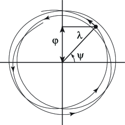
Figure 1: The motion of the pendulum is represented by a point with radius vector $\lambda$ rotating with angular speed $\dot{\psi}$, projected on the vertical axis, so that $\varphi=\lambda\sin\psi$. In this way we achieve that $\varphi=0$ when $\psi$ is an integer multiple of $\pi$. Both $\lambda$ and $\psi$ exhibit slow variations (slower than indicated), resulting in gradual changes in the swing amplitude and the period of the pendulum.

The escapement RAW80 is designed to deliver a torque $m$ that depends only on the angle $\varphi$. It has no intrinsic frequency of its own, but just delivers the torque required by the value of $\varphi$, irrespective of time. So, $m=m(\varphi)$ and Eq. (1) is autonomous. In actual fact $m$ may have a weak dependence on $\dot{\varphi}$ as well. We shall not consider the more general case $m=m(\varphi,\dot{\varphi})$, and we shall take $\varepsilon$ constant. But the theory developed below can handle $\varepsilon$ and $m$ with arbitrary functional dependence on $\varphi$ and $\dot{\varphi}$.

It is straightforward to solve Eq. (1) numerically, but the result contains too much information for our purposes. The time keeping is determined by the times of successive $\varphi=0$ crossings, for which it is sufficient to know $\varphi(t)$ with a time resolution of about a period. In other words, we are interested in slow changes of the amplitude and phase. The problem of gradual secular changes in quasi-periodic systems has come up in physics time and again. One of the earliest applications was the problem of secular perturbations in planetary orbits. AM88 Here we shall follow the theory developed by Krylov, Bogoliubov and Mitropolski (KBM). BM61 ; BLV04 The idea is to take

$$\varphi=\lambda\sin\psi\ ;\quad\dot{\varphi}=\lambda\cos\psi\ ,$$ (2)

where $\lambda$ is the maximum of $\varphi$ (referred to as ‘the amplitude’), and $\psi$ the phase of the pendulum, see Fig. 1. We may regard $\psi$ as the time measured by the pendulum (‘pendulum time’), while $t$ is a stable reference time (‘laboratory time’). One might think that the first relation $\varphi=\lambda\sin\psi$ suffices, for we may compute $\dot{\varphi}=\dot{\lambda}\sin\psi+\lambda\dot{\psi}\cos\psi$ and then $\ddot{\varphi}=\cdots$, insert all that in Eq. (1) and make approximations using $\lambda,\,\varepsilon\ll 1$. However, that path is fraught with ambiguities due to the fact that $\varphi=\lambda\sin\psi$ does not define $\lambda$ and $\psi$ uniquely. We do need a second relation.

II.1 The method of Krylov, Bogoliubov and Mitropolski (KBM)

The next step is to solve Eq. (2) for $\lambda$ and $\psi$,

$$\lambda=(\varphi^{2}+\dot{\varphi}^{2})^{1/2}\ ;\quad\psi=\arctan(\varphi/\dot{\varphi})\ ,$$ (3)

and to compute the derivatives:

$$\dot{\lambda}\! = \!\frac{\varphi\dot{\varphi}+\dot{\varphi}\ddot{\varphi}}{(\varphi^{2}+\dot{\varphi}^{2})^{1/2}}\,=\,\frac{1}{\lambda}\,(\ddot{\varphi}+\varphi)\dot{\varphi}\ ,$$ (4)

$$\dot{\psi}\! = \!\frac{\dot{\varphi}^{2}-\varphi\ddot{\varphi}}{\varphi^{2}+\dot{\varphi}^{2}}\ \ \ \ \ =\,1-\frac{1}{\lambda^{2}}\,(\ddot{\varphi}+\varphi)\varphi\ .\quad$$ (5)

The derivative $\dot{\psi}$ of the phase is the rate at which the pendulum ticks. And ${\textstyle\frac{1}{2}}\lambda^{2}$ is the total (kinetic + potential) energy of the pendulum. Both right hand sides contain $\ddot{\varphi}+\varphi$, which the equation of motion (1) allows us to write as:

$$\ddot{\varphi}+\varphi=-2\varepsilon\dot{\varphi}+(\varphi-\sin\varphi)+m(\varphi)\ .$$ (6)

On the right we recognize the terms responsible for the effects of friction, circular error and driving, respectively. We insert Eq. (6) in Eqs. (4) and (5), and eliminate the remaining $\varphi$ and $\dot{\varphi}$ with the help of Eq. (2):

$$\dot{\lambda}\! = \!-2\varepsilon\lambda\cos^{2}\psi+\{\lambda\sin\psi-\sin(\lambda\sin\psi)\}\,\cos\psi$$ (7)

$$\qquad\qquad\qquad\qquad\qquad+\,m\cos\psi\,,$$

$$\dot{\psi}-1\! = \!2\varepsilon\cos\psi\sin\psi+\{\lambda^{-1}\sin(\lambda\sin\psi)-\sin\psi\}\,\sin\psi$$ (8)

$$\qquad\qquad\qquad\qquad\qquad-\,(m/\lambda)\,\sin\psi\ .$$

Equations (7) and (8) are still equivalent to Eq. (1). KBM then average over one period to remove the fast time scales. This amounts to integrating the equations over $\psi$ over the interval $[\psi_{0}-\pi,\,\psi_{0}+\pi]$ centered at an arbitrary $\psi_{0}$, and to assume that $\varepsilon$, $\lambda$ and $\dot{\psi}$ but not $m$, are constant over one period. Afterwards, the index 0 on $\psi$ is dropped. In doing so, the terms $\{\lambda\sin\psi-\sin(\lambda\sin\psi)\}\,\cos\psi$ in Eq. (7) and $2\varepsilon\cos\psi\sin\psi$ in Eq. (8) vanish because they are antisymmetric in $\psi$. Since $(2\pi)^{-1}\smallint_{-\pi}^{\pi}\cos^{2}\psi\,{\rm d}\psi={\textstyle\frac{1}{2}}$ we obtain:

$$\dot{\lambda} = -\varepsilon\lambda+\oint\,m(\varphi)\cos\psi\,{\rm d}\psi\,+\,O_{1}(\varepsilon^{2})\ ,$$ (9)

$$\dot{\psi}-1 = -\frac{1}{16}\,\lambda^{2}-\frac{1}{\lambda}\,\oint\,m(\varphi)\sin\psi\,{\rm d}\psi\,+\,O_{2}(\varepsilon^{2})\ ,\quad$$ (10)

where we use the notation $\oint=(2\pi)^{-1}\smallint_{-\pi}^{\pi}\,$. We demonstrate in appendix A how the circular error term $-\lambda^{2}/16$ is extracted from Eq. (8).

In reality $\varepsilon$, $\lambda$ and $\dot{\psi}$ are not constant over a period. Bogoliubov and Mitropolski BM61 show that this produces correction terms in Eqs. (9) and (10) having the form of a power series in $\varepsilon$. These higher order terms play no role here, except in Sec. VI where we believe to observe the effect of the lowest order terms $\propto\varepsilon^{2}$.

Briefly, what if $\varepsilon$ and $m$ depend on $\varphi$ and $\dot{\varphi}$? Take for example $\varepsilon$. Then set $\varepsilon=\varepsilon(\varphi,\dot{\varphi})=\varepsilon(\lambda\sin\psi,\lambda\cos\varphi)$ in Eqs. (7) and (8). The average over a period will now generate a friction-like term in the rate equation (10), etc.

III The physics of eqs. (9) and (10)

Equations (9) and (10) are first order ODEs well-suited for a study of the long-term dynamics of the pendulum. Equation (9) determines the amplitude $\lambda$ and the total energy $\lambda^{2}/2$ of the pendulum. The amplitude changes only slowly because the friction time scale $\varepsilon^{-1}$ is long, $1/(2\pi\varepsilon)$ nominal periods, and because the escapement needs to deliver many small kicks to alter the energy ${\textstyle\frac{1}{2}}\lambda^{2}$. The damping is compensated by the driving term $\oint m\cos\psi\,{\rm d}\psi$. A back-of-the-envelope derivation of Eqs. (9) and (10) is given in appendix B.

III.1 The rate equation (10)

Equation (10) for the rate features the circular error term $-\lambda^{2}/16$, due to the difference between $\varphi$ and $\sin\varphi$ in Eq. (6). It has a minus sign because the circular error increases the period, so it must reduce the rate. Friction does not appear, and has therefore only an indirect effect on the rate through its influence on $\lambda$.

The term $-\lambda^{-1}\oint m\sin\psi\,{\rm d}\psi$ is called the escapement error. It specifies the relative rate change induced by a driving torque $m$, as computed already by Airy GBA30 . The history of horology is to a large extent a quest for technical solutions to make this term and the circular error as small as possible.

An important feature of both equations is that the driving torque $m$ appears only in the form of two averages over a period. This is a consequence of the elimination of fast time scales and demonstrates that much of the fine structure in the driving torque averages out and is irrelevant for the pendulum’s long term dynamics. Only two numbers matter, namely the even (cosine) and odd (sine) moment, and all pendulums with escapements having the same $\oint m\cos\psi\,{\rm d}\psi$ and $\oint m\sin\psi\,{\rm d}\psi$ are in principle equivalent time keepers.

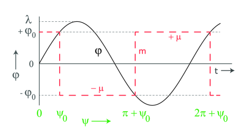
Figure 2: The model escapement delivers a constant torque $m=\mu$, switching to $m=-\mu$ after half a period ($-\;-\;-$). The switch is at a fixed pendulum angle $\varphi_{0}$ in the first quarter of the swing, and $-\varphi_{0}$ in the third. The phase $\psi$ is indicated at the bottom.

III.2 A model escapement

For our numerical work we introduce a simple escapement, see Fig. 2 and Woodward W06chap2 . A constant driving torque $m=\mu>0$ switching to $m=-\mu$ after half a period, and so on. The switch is at a fixed (mechanically determined) pendulum angle $\varphi_{0}$. The phase $\psi_{0}$ at that moment depends on the amplitude according to Eq. (2):

$$\varphi_{0}=\lambda\sin\psi_{0}\ ;\qquad 0<\psi_{0}<\pi/2\ .$$ (11)

The swing amplitude $\lambda$ must be larger than $\varphi_{0}$, otherwise the driving torque cannot switch sign, and the pendulum will stall. Since $\varphi_{0}=\lambda\sin\psi_{0}$ has two solutions, $\psi_{0}$ and $\pi-\psi_{0}$, we impose $0<\psi_{0}<\pi/2$ because escapements generally switch to a torque counteracting the motion before the pendulum reaches maximum amplitude.

Actual escapements deliver a more complicated $m$, MK78 ; MS06 ; MWV12 but as argued above, this fine structure of $m$ is expected to be relatively unimportant for the performance. So we hope to catch the main features of this and similar escapements with the help of this simple model. We compute the two averages required in Eqs. (9) and (10):

$$a\! \equiv \!\!\oint m\,\cos\psi\,{\rm d}\psi$$

$$= \!\!\frac{1}{2\pi}\,\bigg{\{}-\int_{\psi_{0}}^{\pi+\psi_{0}}+\int_{\pi+\psi_{0}}^{2\pi+\psi_{0}}\bigg{\}}\,\mu\cos\psi\,{\rm d}\psi$$

$$= \!\!\frac{2\mu}{\pi}\,\sin\psi_{0}\,=\,\frac{2\mu\varphi_{0}}{\pi\lambda}\ .$$ (13)

Since the integrand is a periodic function of $\psi$ we may start the integration where we like, as long as we integrate over a full period. A similar computation yields

$$b\equiv\oint m\,\sin\psi\,{\rm d}\psi=-\,\frac{2\mu}{\pi}\,\cos\psi_{0}\ .\qquad\ \$$ (14)

Equations (9) and (10) for the amplitude and the phase may now be written as:

$$\frac{{\rm d}\lambda^{2}}{{\rm d}t} = -2\varepsilon\lambda^{2}+\frac{4\mu\varphi_{0}}{\pi}\,+\,O_{1}(\varepsilon^{2})\ ,$$ (15)

$$\dot{\psi}-1 = -\frac{1}{16}\,\lambda^{2}+\frac{2\mu}{\pi\lambda}\,\cos\psi_{0}\,+\,O_{2}(\varepsilon^{2})\ ,\quad$$ (16)

where Eq. (16) may be further reduced with $\cos\psi_{0}=[1-(\varphi_{0}/\lambda)^{2}]^{1/2}$, as follows from Eq. (11). Due to a different notation the escapement error does not look like any of the expressions in Ch. 7 of Rawlings RAW80 . But we have verified that we can reproduce these formulae starting from our expressions $[2\mu/(\pi\lambda)]\,\cos\psi_{0}$ in Eq. (16) or $-(1/\lambda)\oint m\sin\psi\,{\rm d}\psi$ in Eq. (10). So the difference is only apparent. In appendix C we analyse the action of an escapement that delivers a single impulse in each period.

III.3 Analytic solution

Before we start using Eqs. (15) and (16), we point out that they often possess a simple analytic solution, which may be useful in theoretical investigations. For example, if $\varepsilon$ is constant and the transient responses are over, the system is in a quasi-stationary state and the solution of Eq. (15) is:

$$\lambda^{2}=\frac{4\varphi_{0}}{\pi}\int_{0}^{\infty}\exp(-2\varepsilon\tau)\,\mu(t-\tau)\,{\rm d}\tau\ .$$ (17)

This permits us to compute $\lambda(t)$ for any time-dependent driving torque $\mu(t)$. And once $\lambda$ is known, we may compute $\dot{\psi}$ from Eq. (16). For example, let there be a jump in $\mu$ at $t=0$ and $\mu=\mu_{0}$ for $t<0$ and $\mu=\mu_{1}$ for $t>0$. Inserting that in Eq. (17) produces

$$\lambda^{2}\,=\,\frac{2\varphi_{0}}{\pi\varepsilon}\cdot\left\{\!\begin{array}[]{ll}\mu_{0}&\ t<0\ ,\\[8.53581pt] \{\mu_{1}-(\mu_{1}-\mu_{0})\exp(-2\varepsilon t)\}&\ t>0\ .\end{array}\right.$$ (18)

This result will be used later to explain the numerical work in Sec. V. Just replace $t$ by $t-t_{0}$ everywhere in Eq. (18) if the jump is at $t_{0}$.

Figure 3: Contour plot of $\dot{\psi}-1$ in sec/day as a function of $\varepsilon$ and $\mu$, for $\varphi_{0}=0.03\cong 1.7^{\circ}$. This is the rate in excess of the nominal rate of a pendulum driven by the model escapement. Lines of constant swing amplitude are dotted, $\lambda=\varphi_{0}$ and higher up $2\varphi_{0}$ and $3\varphi_{0}$. For example, if $\varepsilon\sim 5\times 10^{-5}$ and $\mu\sim 10^{-5}$, the pendulum loses about $10\,$s per day with respect to the nominal rate, and the swing amplitude is about $2\varphi_{0}$. Further details in main text.

IV Stationary operation

The asymptotic theory developed above enables us to address many questions that would be difficult to answer if we had only the equation of motion (1). We begin with the case that $\varepsilon$, $\mu$ and $\varphi_{0}$ are constant. The pendulum will then perform stationary oscillations after some time. We study how the stationary amplitude $\lambda$ and rate $\dot{\psi}$ depend on the parameters. The amplitude follows by setting ${\rm d}\lambda^{2}/{\rm d}t=0$ in Eq. (15):

$$\lambda=\varphi_{0}\bigg{(}\frac{2\mu}{\pi\varepsilon\varphi_{0}}\bigg{)}^{1/2}\ ,$$ (19)

and using this in Eq. (16) we obtain the stationary rate:

$$\dot{\psi}-1\,=\,-\,\frac{\mu\varphi_{0}}{8\pi\varepsilon}\,+\,\varepsilon\bigg{(}\frac{2\mu}{\pi\varepsilon\varphi_{0}}-1\bigg{)}^{1/2}.$$ (20)

The first term on the right is the circular error (no longer readily recognizable as such). It is negative and reduces the rate. The second term is the escapement error, which is manifestly positive. It follows that the driving necessary to keep the pendulum going, always forces it to run a little faster as well. This confirms one’s intuition, and the physical reason is, loosely speaking, that during most of the time the escapement is pushing the pendulum ever so gently forward. These statements hold for the model escapement and comparable types, e.g. the recoil escapement, W06recoil but not for all, see appendix C.

Fig. 3 shows the excess rate on top of the nominal rate $\dot{\psi}=1$ in sec/day due to circular and driving error together. The $\varepsilon$-$\mu$ plane is divided in three regions:
1. A losing rate, to the left and up. In this region the amplitude $\lambda$ is large because the friction is relatively small. As a result, the circular error is larger than the escapement error, and the pendulum rate is sub-nominal.
2. A gaining rate, to the right and up: here the effect of the driving torque dominates (escapement error). These regions are separated by the dashed contour where circular and escapement error compensate each other. Pendulums operating on this dashed line run at nominal rate.
3. In the third region, below the line $\lambda=\varphi_{0}$, the driving is too weak to keep the swing amplitude $\lambda$ above the value $\varphi_{0}$, and the pendulum stalls. The minimum required torque $\mu$ is ${\textstyle\frac{1}{2}}\pi\varepsilon\varphi_{0}$.

IV.1 Losing or gaining?

Here comes a perennial question: will a clock lose or gain when a parameter is changed? Take for example the driving torque. The discussion usually proceeds as follows: $\mu\uparrow$ implies a larger amplitude $\lambda$, which means a larger circular error, i.e. $\dot{\psi}\downarrow$. But sometimes we observe the opposite. How come? On closer look, the answer depends on the pendulum’s initial operating point in Fig. 3. If that is towards the left where the circular error dominates, then $\mu\uparrow$ makes the first term (circular error) in Eq. (20) go down and $\dot{\psi}\downarrow$. But if we start more to the right where the escapement error dominates, the second term in Eq. (20) (escapement error) increases. So $\dot{\psi}\downarrow$ when we start on the left in Fig. 3, but $\dot{\psi}\uparrow$ when we begin on the right. There is no simple answer.

Variations in friction may be dealt with in the same manner. A remarkable feature is that the pendulum may run faster when friction is increased. Take for example $\mu$ fixed at $2\times 10^{-5}$ in Fig. 3, then the rate goes up with $\varepsilon$ until $\varepsilon\sim 2.5\times 10^{-4}$ and decreases only thereafter.

IV.2 Accuracy

The accuracy of the time keeping is a subject with many different aspects, of which we shall discuss only one. Experience has shown that the accuracy of a pendulum is largely set by the friction coefficient $\varepsilon$. The driving plays a minor role. Why is that so? The answer comes in two steps.

We focus on long time scales ($\gg\varepsilon^{-1}$). In that case we may ignore the time derivative in Eq. (9) and obtain the following order-of-magnitude estimate: $\varepsilon\lambda\sim m$, or $m/\lambda\sim\varepsilon$, which we use to estimate $\dot{\psi}-1$ with Eq. (10):

$$\dot{\psi}-1\,\sim\,m/\lambda\,\sim\,\varepsilon\ .$$ (21)

Here we assume that the pendulum operates in region 2 of Fig. 3 where the circular error is negligible. Thus we have found that $\dot{\psi}-1\sim\varepsilon$, and Eq. (20) is basically telling the same story. The point is that the driving torque no longer appears in Eq. (21) because it could be approximately eliminated by requiring quasi-stationary operation.

The second part of the answer is that as long as the parameters are constant, nothing changes. The rate is exactly constant and the pendulum is a perfect time keeper, even though it may not run at nominal rate. But parameters are never constant and change on a variety of time scales. Experience has shown that changes of several tens of percent in the parameters and more are not uncommon. And that makes $\varepsilon$ a reasonable upper limit for the relative precision of the pendulum rate.

IV.3 Optimal driving torque

From Eqs. (9) and (10) the least disturbing driving torque is seen to be an impulse in a narrow phase interval $\delta\psi\ll 1$ centered at $\psi=k\pi$, when the pendulum passes through its equilibrium position $\varphi=0$. The escapement error is then $\lambda^{-1}\oint m\sin\psi\,{\rm d}\psi\sim(m/\lambda)(\delta\psi)^{2}\sim\varepsilon\delta\psi$. Here we used that $m\delta\psi\sim\varepsilon\lambda$, as follows from Eq. (9). We conclude that it should be possible to beat the precision estimate (21) by a factor $\delta\psi\ll 1$, with the help of a specially designed escapement. All this is well known - we merely illustrate that the present formulation which uses concepts that are close to the instrument, allows a more direct answer to such questions than Eq. (1) alone.

Figure 4: Numerically determined pendulum angle $\varphi$. On the horizontal axis time in nominal periods. Parameters: $\varepsilon=2.5\times 10^{-4}$, $\varphi_{0}=0.03$, timestep $dt=0.03$. Initial conditions: $\varphi(0)=0$, $\dot{\varphi}(0)=(2\mu_{0}\varphi_{0}/\pi\varepsilon)^{1/2}$ (stationary swing). At $t/2\pi=150$ the driving torque switches from $\mu_{0}=2\times 10^{-5}$ to $\mu_{1}=4\times 10^{-5}$. There is no visible reaction.

V Transient effects

We validate the asymptotic theory developed above with two case studies. The first is the reaction of the pendulum to a jump in the driving torque. We solve Eq. (1) numerically, parameters as in Fig. 4; for details see appendix D. The pendulum is set off in a stationary swing, and the value of $\dot{\varphi}(0)$ follows from Eq. (3): $\dot{\varphi}(0)=\lambda$ and $\lambda$ may be had from Eq. (19). There are $2\pi/dt\sim 209$ time steps in one nominal period. A similar numerical experiment has been carried out by Woodward. W06sim

The solution, Fig. 4, is not very telling: a series of identical oscillations, and there is no visible reaction in the vicinity of the jump in $\mu$ at $t/2\pi=150$. To refine the analysis we determine the times $t_{i}$ that $\varphi(t)$ crosses zero (from $-$ to $+$). Numerical details are given in appendix D. Since $\psi$ increases by $2\pi$ at each next zero $i$ of $\varphi$ (by definition), we may determine the time (i.e. phase) $\psi$ and the rate $\dot{\psi}$ measured by the pendulum on a non-equidistant grid $\{t_{i}\}$, as follows:

$$\psi_{i}=2\pi i\,;\qquad\dot{\psi}_{i}=2\pi(t_{i}-t_{i-1})^{-1}\ .$$ (22)

This procedure can be easily implemented in the numerical model (and in a pendulum experiment). The measured rates may then be confronted with theory, Eq. (16).

The reaction of the pendulum, Fig. 5, top panel, is now clearly visible. The initial operating point of the pendulum is $A$ in Fig. 3, where it gains about $1.1\times 10^{-4}$ or $\sim 10$ sec/day. The rate changes instantaneously, together with the jump in the driving, and then tapers off to a new stationary value $\sim 2\times 10^{-4}$ or $\sim 17$ s/day in the new operating point $B$. The time scale is set by $\lambda$, Fig. 5, bottom panel, and $\lambda$ changes only slowly because it takes many small pushes of the escapement to change the energy $\lambda^{2}/2$. Once $\lambda$ is known, we compute $\dot{\psi}-1$ with Eq. (16), as a verification. A few values are displayed as $\diamond$ in Fig. 5.

The magnitude of the rate jump follows directly from Eq. (16): since $\lambda$ changes slowly, and $\cos\psi_{0}$ depends only on $\lambda$, the rate difference just before and after the jump is $\delta\dot{\psi}=2(\delta\mu)\cos\psi_{0}/(\pi\lambda)$. This allows us to compute that $\dot{\psi}-1=3.2\times 10^{-4}$ after the jump, as observed. The jump in the rate is tiny but well measurable. It is an arresting experience for students experimenting with a pendulum in a practical physics course. The unaided eye sees no change when the driving is altered, and yet it happens, just because the escapement pushes a little harder.

Figure 5: Reaction of the pendulum to a jump in the driving torque (parameters as in Fig. 4). On the horizontal axis time in nominal periods. At $t/2\pi=150$ the driving torque switches from $\mu_{0}=2\times 10^{-5}$ to $\mu_{1}=4\times 10^{-5}$. Top panel: excess rate of the pendulum (in seconds per sec), as ‘observed’, that is, computed from definition (22). The noise on the rate curve is numerical and can be reduced by taking a smaller timestep $dt$. Diamonds $\diamond$ are values inferred from theory, Eq. (16). Bottom panel: amplitude $\lambda$ computed from Eq. (3) and the simulation data; Eq. (18) yields the same result.

Finally, we compute the time shift the pendulum incurs. Locating the jump for simplicity at $t=0$, the phase shift is $\Delta\psi=\int_{0}^{\infty}(\dot{\psi}-\dot{\psi}_{\rm r})\,{\rm d}t$, where $\dot{\psi}$ is the rate given by Eq. (16) using Eq. (18) for $\lambda$, and $\dot{\psi}_{\rm r}$ the constant rate of a reference pendulum operating in point $B$, i.e. the area under the curve $\dot{\psi}$ and above the tangent to $\dot{\psi}$ in $t=\infty$. We find $\Delta\psi=0.295$, or $(\Delta\psi/2\pi)\cdot 2\,$s $\sim 0.1\,$s for a $1\,$m pendulum.

We have also looked at the pendulum’s reaction to sudden changes in $\varepsilon$. The main difference is that the rate no longer makes a sudden jerk but adapts slowly to its final value, like $\lambda$ does. In conclusion we can say that the asymptotic theory seems to work well, also for a rapid change as we encountered here.

VI Long-term behavior

The second case study is a pendulum with a variable driving torque, running at nominal rate in point $C$ in Fig. 3 in the absence of variability. The co-ordinates of $C$ are $\mu_{0}=1.5\times 10^{-5}$ and $\varepsilon=1.167245\times 10^{-4}$ (obtained by solving Eq. (16) for $\varepsilon$ with $\dot{\psi}=1$ and $\mu_{0}=1.5\times 10^{-5}$).

The reason for selecting this model is not because we think it is particularly realistic, but because we need a ‘rough’ test bed to see how well the data generated by the ‘numerical clock’, i.e. Eqs. (1) and (23), are recovered by the theoretical model, i.e. Eqs. (15) and (16) together with (23).

The simulation advances Eq. (1) for $10^{9}$ timesteps ($dt=0.03$), comprising $\sim 4.8\times 10^{6}$ nominal periods, or about 110 days for a $1\,$m pendulum. The initial conditions are as in Fig. 4 (stationary swing). During the simulation we determine the $-+$ zero crossing times $\{t_{i}\}$ of $\varphi$ and the pendulum time $\psi_{{\rm p},i}$ at these moments, basically by counting sine waves, see definition (22). We also integrate Eqs. (15) and (16) on this $\{t_{i}\}$ grid, to determine the model pendulum time $\psi_{{\rm m},i}$.

The driving torque $\mu$ has a random component:

$$\mu=\mu_{0}\,\{1+\delta\mu(t)/\mu_{0}\}\ ,$$ (23)

where $\delta\mu(t)$ is a normally-distributed random variable with zero mean and variance $\delta\mu_{\rm r.m.s.}^{2}$ that is renewed at every $-+$ zero crossing of $\varphi$. The coherence or correlation time of $\delta\mu(t)$ is therefore one nominal period.

In spite of the location of $C$ in Fig. 3, the pendulum does not run at nominal rate. In the absence of variability it gains $\sim 0.005/5\times 10^{-5}=10^{-8}$, or $\sim 0.3\,$s/yr, see Fig. 6, top panel. This is ten times better than the performance of a Shortt clock, see Ref. RAW80, , p. 126. The effect is therefore extremely small, but we discuss it because we are after long-term effects here. Otherwise, the pendulum is seen to be almost impervious to the large variability in the driving, with an r.m.s. gain of $\sim 0.04/4\times 10^{6}\sim 10^{-8}$, or $\sim 0.3\,$s/yr (same number by coincidence).

Why is it so insensitive to the fluctuations? The decisive factor is the fact that the variations are fast, $\delta\mu(t)$ being renewed after each period, while the pendulum has a long memory $\sim\varepsilon^{-1}$, i.e. many periods. So there is a considerable cancellation of the random component of $\mu$.

Slow variability however (time scale much larger than the period), results in little cancellation, so that the pendulum is quite sensitive to this type of variability. Basically, we rediscover here what horologists have known for a long time: accurate time keeping is all about controlling and eliminating slow, low-frequency variations in the parameters. Fast variations are much less detrimental.

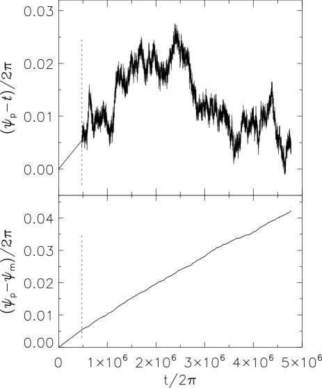
Figure 6: Simulation of the pendulum motion comprising $10^{9}$ timesteps, or $10^{9}\,dt/2\pi\sim 4.8\times 10^{6}$ nominal periods, about $110$ days for a $1\,$m pendulum. Shown is the difference between pendulum time $\psi_{\rm p}$ and laboratory time $t$ (top), and between pendulum time $\psi_{\rm p}$ and model pendulum time $\psi_{\rm m}$ (bottom), as a function of laboratory time. To reduce blackening only one out of every 500 data points is plotted. Parameters: $\mu_{0}=1.5\times 10^{-5},\ \varepsilon=1.167245\times 10^{-4},\ \varphi_{0}=0.03,\allowbreak\ dt=0.03,\ \delta\mu_{\rm r.m.s.}=0.3\,\mu_{0}$. The random component $\delta\mu(t)$ in the driving is switched on beyond the dotted line ($t/2\pi>4.8\times 10^{5}$). The simulation took $10^{4}\,$s (double precision IDL).

Returning to the main question, how well do Eqs. (15) and (16) model the pendulum dynamics? The bottom panel of Fig. 6 shows that the strong variability of pendulum time $\psi_{\rm p}$ seen in the top panel and induced by the driving noise, is by and large correctly modeled in $\psi_{\rm m}$ and removed. Only this small secular difference of $\sim 10^{-8}$ remains. We ran other simulations, and all graphs of $\psi_{\rm p}-\psi_{\rm m}$ versus $t$ looked more or less the same. This suggests that we see the effect of the $O_{2}(\varepsilon^{2})$ term in Eq. (16), a term that we cannot model out as its theoretical form is unknown.BM61 ; BLV04 Perhaps we see the second-order correction $-{\textstyle\frac{1}{2}}\varepsilon^{2}$ of the oscillator frequency. LL78 That has the right order of magnitude and sign since $-{\textstyle\frac{1}{2}}\varepsilon^{2}\sim-10^{-8}$.

Our conclusion is that also in this case the asymptotic theory appears to work well. Equations (15) and (16) deliver a relative rate precision of $\sim\varepsilon$ or better. This suffices for a physical pendulum as that attains a precision of $\sim\varepsilon$ anyway (Sec. IV.2). In numerical experiments where one may switch on and off perturbations at liberty, there may be cases that require computation and inclusion of the second order terms $O_{1}$ and $O_{2}$.

VII Concluding remarks

The purpose of this study is to demonstrate that the long-term dynamics of a pendulum as typically used in clocks can be simulated efficiently with two first order ODEs, Eq. (15) for the amplitude $\lambda$ and Eq. (16) for the phase $\psi$ of the pendulum. By using the rate $\dot{\psi}$ instead of its inverse (the period) and by averaging over fast time scales, we obtain simple model equations (15) and (16) that show that the effects of driving, friction and circular error are additive. In this way we could deduce the expressions for these effects in a unified framework, without any reference to a phase diagram (Ref. RAW80, , Ch. VII). In particular, the derivation of the escapement error in Eq. (10) runs smoothly and is free of ad hoc assumptions.

We employ the method of Bogoliubov and Mitropolski BM61 ; BLV04 , which involves averaging over a pendulum period. Time scales smaller than a period can no longer be resolved, but these are not important for the time keeping properties of the pendulum. The pleasant consequence is that the model equations are rather insensitive to fine structure in the driving torque $m(\varphi)$, which in turn allows us to use a simple model escapement. It is no longer necessary to resolve individual pendulum swings in small timesteps - we may now make timesteps of one pendulum period, resulting in a considerable time saving, and the possibility to make long simulations with all effects acting simultaneously.

We studied two examples with the equation of motion (1) and compared the results with those of the model equations (15) and (16): a sudden change in the driving torque and a permanently noisy driving. Satisfactory agreement was found. More complete models need to consider other disturbing factors; we only mention here that slow length changes $\delta\ell(t)$ of the pendulum produce an extra term $-\delta\ell/2\ell_{0}$ on the right of Eqs. (10) and (16), while Eqs. (9) and (15) for the amplitude remain unchanged ($\ell_{0}$ is the nominal pendulum length). If necessary new model equations may be derived for special escapements, see e.g. Eqs. (28) and (29).

Now that the validation has been done, the road is open to fast simulations with the model equations (15) and (16). For example, the simulation of Fig. 6 comprises $\sim 110$ days for a $1\,$m pendulum. It took $10^{4}\,$s with the equation of motion (1), but only $\sim 50\,$s with the model equations (15) and (16). Note that the reliability of such long-duration simulations is limited by the unknown influence of the second order terms. Evaluation of these second order terms seems to be an interesting topic now.

It is evident from Eqs. (9) and (10) that any fine structure of the type $\sum_{n\neq 1}(a_{n}\cos n\psi+b_{n}\sin n\psi)$ may be added to $m(\varphi)$ without affecting the time keeping. This opens the door to a wide variety of equivalent shapes for the driving torque $m$. But if the shape of $m$ is so unimportant, why did clockmakers bother to refine escapements? The answer must be that when parameters change and adapt to the environment, it is very difficult not to change the two quantities $\oint m\cos\psi\,{\rm d}\psi$ and $\oint m\sin\psi\,{\rm d}\psi$ that are crucial for the time keeping. The best strategy seems to be to reduce $\varepsilon$ as much as possible.

A pendulum is the archetype harmonic oscillator, an omnipresent system in physics with widely different appearances. BB05 Laboratory experiments with a driven, damped oscillator are therefore of permanent educational value. These need not be restricted to a pendulum. One might try for example a quartz crystal or any kind of electronic oscillator. But whatever the nature of the oscillator, the unifying concept of a driven, damped, restlessly swinging pendulum is likely to keep physicists and horologists spellbound forever.

Appendix A The circular error

The circular error term follows from Eq. (8):

$$\!\!{\rm\ circ.\ error}\!\! = \!\!\oint\{\lambda^{-1}\sin(\lambda\sin\psi)-\sin\psi\}\sin\psi\,{\rm d}\psi$$ (24)

$$= \!\frac{1}{\lambda}\,J_{1}(\lambda)-\frac{1}{2}\,\,\simeq\,\!-\frac{1}{16}\,\lambda^{2}+\frac{1}{384}\,\lambda^{4}\,\cdot\cdot\,.\qquad$$

Here, $J_{1}$ is a Bessel function of the first kind. AS68 The essential steps in the computation above are (a) to use for $\sin(\lambda\sin\psi)$ relation 9.1.43 of Ref. AS68, , and then (b) the expansion $J_{1}(\lambda)=x(1-x^{2}/2+x^{4}/12-\cdots)$ with $x=\lambda/2$, cf. relation 9.1.10 of Ref. AS68, .

We present Eq. (24) here because it differs from the usual expansions (e.g. Ref. RAW80, , p. 51 and Ref. NO86, , Eq. (8). This is because Eq. (24) specifies the effect of circular error on the rate, not on the period.

Appendix B Back-of-the-envelope derivation of equations (9) and (10)

The power fed into the pendulum is torque $\times$ angular speed $=m\dot{\varphi}=m\lambda\cos\psi$ (use Eq. (2) for $\dot{\varphi}$; gravity does on average no work). But this is also the time derivative of the total energy, so ${\rm d}({\textstyle\frac{1}{2}}\lambda^{2})/{\rm d}t=m\lambda\cos\psi$ or $\dot{\lambda}=m\cos\psi$. Eq. (9) follows by adding friction and averaging.

Suppose $m$ is a single impulse. At that instant $\dot{\varphi}$ gets a boost while $\varphi=\lambda\sin\psi$ is constant, so $0={\rm d}(\lambda\sin\psi)/{\rm d}t=\dot{\lambda}\sin\psi+\lambda\dot{\psi}\cos\psi$. Solve for $\dot{\psi}$ and insert $\dot{\lambda}=m\cos\psi$ to obtain $\dot{\psi}=-(m/\lambda)\sin\psi$. This is the core of Eq. (10). Add all impulses $m_{i}$ composing $m$ in one period: $\delta^{\prime}\psi=\allowbreak\sum\delta\psi_{i}=\allowbreak-(1/\lambda)\sum m_{i}\sin\psi_{i}\,\delta t=\allowbreak-(1/\lambda)\int m\sin\psi\,{\rm d}t$ ($\lambda$ is constant over a period). Denote the mean time derivative of $\psi$ again by $\dot{\psi}$, then $\dot{\psi}\simeq\delta^{\prime}\psi/2\pi\simeq-(1/\lambda)\int m\sin\psi\,{\rm d}t/2\pi\,\simeq-(1/\lambda)\oint m\sin\psi\,{\rm d}\psi$ (since ${\rm d}\psi/{\rm d}t=1+{\rm small\ terms}$, so ${\rm d}t\simeq{\rm d}\psi$). Finally, add the nominal rate $\dot{\psi}=1$, and the circular error $-\lambda^{2}/16$.

It is hoped that these informal arguments help to clarify those of Ref. RAW80, , Ch. 7 and Woodward. W76

Appendix C A single-impulse escapement

The model escapement, Fig. 2, that we have used sofar interferes continuously with the pendulum motion. Here we compare it with an escapement of opposite type, that delivers in each period a single impulse at a fixed pendulum angle $\varphi_{1}$:

$$m(\varphi)=e\,\delta(\varphi-\varphi_{1})\ .$$ (25)

The function $\delta(x)$ is basically a sharp peak at $x=0$. Width and height are inversely proportional such that $\int\delta(x-x_{0})\,{\rm d}x=1$, provided $x_{0}\in I,$ the integration interval. The width of $\delta(x)$ is supposed to be much smaller than all fine structure in the problem at hand, whence $\int f(x)\delta(x-x_{0})\,{\rm d}x\simeq f(x_{0})$ if $x_{0}\in I$, otherwise zero.

The energy transferred to the pendulum in one period is $\int m\,{\rm d}\varphi=e>0$. It follows that ${\rm d}\varphi>0$ at $\varphi_{1}$, i.e. $\varphi$ is increasing. Since $\varphi_{1}=\lambda\sin\psi_{1}$ according to Eq. (2), the phase $\psi_{1}$ at the impulse is in the 1st or 4th quadrant. We compute $a$ and $b$ given by Eqs. (III.2) and (14):

$$b=\oint m\sin\psi\,{\rm d}\psi=\frac{e}{2\pi}\int_{-\pi}^{\pi}\delta(\varphi-\varphi_{1})\sin\psi\,{\rm d}\psi\ .$$ (26)

Here we hit a technicality: to be able to apply the $\delta$-function recipe we transform the integration over $\psi$ to one over $\varphi$. From $\varphi=\lambda\sin\psi$ and $\lambda\simeq$ constant in a period, we infer ${\rm d}\psi=({\rm d}\varphi/{\rm d}\psi)^{-1}{\rm d}\varphi=\allowbreak(\lambda\cos\psi)^{-1}{\rm d}\varphi$, so

$$b=\frac{e}{2\pi\lambda}\int_{-\lambda}^{\lambda}\tan\psi\;\delta(\varphi-\varphi_{1})\,{\rm d}\varphi=\frac{e}{2\pi\lambda}\,\tan\psi_{1}\ .$$ (27)

A similar computation yields $a=e/(2\pi\lambda)$. To obtain the new model equations for $\lambda$ and $\psi$ we repeat the calculation of Sec. III.2, resulting in:

$$\dot{\lambda}\! = \!-\varepsilon\lambda+\frac{e}{2\pi\lambda}\ ,$$ (28)

$$\dot{\psi}-1\! = \!-\frac{\lambda^{2}}{16}-\frac{e}{2\pi\lambda^{2}}\,\tan\psi_{1}\ .$$ (29)

These equations may be used to study the performance of a single-impulse escapement. We briefly look at the case of stationary operation. The amplitude is then $\lambda=(e/2\pi\varepsilon)^{1/2}$ and the rate is:

$$\dot{\psi}-1=-\frac{e}{32\pi\varepsilon}-\varepsilon\tan\psi_{1}\ .$$ (30)

The last term is the escapement error, which now either increases the rate ($\psi_{1}<0$, impulse before a zero), or reduces it ($\psi_{1}>0$, impulse after a zero), cf. Ref. RAW80, , p. 130. Note that $\varphi_{1}=\lambda\sin\psi_{1}$ implies $\tan\psi_{1}=\varphi_{1}(\lambda^{2}-\varphi_{1}^{2})^{-1/2}$, and just as in Eq. (16), we see the appearance of the square root functions in Ch. VII of Ref. RAW80, .

Appendix D Numerical issues

We rewrite Eq. (1) as a first order ODE in the variable $(\varphi,\dot{\varphi})$ which we solve with the IDL routine RK4. To model the escapement the code finds out, at each timestep, in which quadrant $\varphi$ lies (from the signs of $\varphi$ and $\dot{\varphi}$). From the values of $\varphi$ and $\varphi_{0}$ the code then decides between $m=+\mu$ and $m=-\mu$, according to Fig. 2.

The simulation delivers pendulum angles $\varphi_{k}$ on an equidistant grid $t_{k}$, stepsize $dt$. To measure the rate with Eq. (22) we need the $-+$ zero crossing times of $\varphi$ with a precision much better than $\sim\varepsilon$. This follows from Eqs. (21) and (22). It is therefore necessary to do the whole (IDL) simulation in double precision. The timestep $k$ enclosing a zero obeys $\varphi_{k-1}<0$ and $\varphi_{k}>0$. An approximate zero crossing time is found by linear interpolation: $t_{\rm zero}=t_{k-1}+dt\cdot\varphi_{k-1}/(\varphi_{k-1}-\varphi_{k}$). This gave an acceptable accuracy, though we do observe some numerical noise, for example in Fig. 5, top panel.

References

- (1) A.L. Rawlings, The science of clocks and watches (EP Publishing Ltd, Wakefield, UK, 1980).
- (2) B. Taylor and the BHI, “Woodward on time - a compilation of Philip Woodward’s horological writings,” (Associated Agencies Ltd., Oxford, 2006).
- (3) G.L. Baker and J.A. Blackburn, The Pendulum - a case study in physics (Oxford UP, UK, 2005).
- (4) C. Gauld, “Pendulums in the physics education literature: a bibliography,” Science Educat. 13, 811-832 (2004).
- (5) G.B. Airy, “On the disturbances of pendulums and balances and on the theory of escapements,” Trans. Camb. Phil. Soc. III, Part I, 105-128 (1830).
- (6) M. Kesteven, “On the mathematical theory of clock escapements,” Am. J. Phys. 46, 125-129 (1978).
- (7) R.A. Nelson and M.G. Olsson, “The pendulum - Rich physics from a simple system,” Am. J. Phys. 54, 112-121 (1986).
- (8) M. Denny, “The pendulum clock: a venerable dynamical system,” Eur. J. Phys. 23, 449-458 (2002).
- (9) A.A. Andronov, A.A. Vitt and S.E. Khaikin, Theory of oscillators (Pergamon Press, Oxford, 1966), pp. 146-208.
- (10) D. Moline, J. Wagner and E. Volk, “Model of a mechanical clock escapement,” Am. J. Phys. 80, 599-606 (2012).
- (11) F.C. Moon and P.D. Stiefel, “Coexisting chaotic and periodic dynamics in clock escapements,” Phil. Trans. R. Soc. A 364, 2539-2564 (2006).
- (12) R.J. Matthys, Accurate clock pendulums (Oxford UP, 2007).
- (13) See e.g. A. Milani, “Secular perturbations of planetary orbits and their representation as series,” in Long-Term Dynamical behaviour of natural and artificial N-Body Systems, edited by A.E. Roy (Kluwer, 1988), 73-108.
- (14) N.N. Bogoliubov and Y.A. Mitropolski, Asymptotic methods in the theory of non-linear oscillations (Hindustan Publ. Corp., 1961).
- (15) F. Bouziani, I.D. Landau, A. Voda-Besançon, First and second-order K-B approximations for the analysis of nonlinear oscillations in autonomous systems (Technical Report, Laboratoire d’Automatique de Grenoble at ENSIEG, INPG, June 11, 2004).
- (16) see Ref. W06, , p. 59-124.
- (17) see Ref. W06, , p. 71.
- (18) see Ref. W06, , p. 108-114.
- (19) L.D. Landau and E.M. Lifshitz, Mechanics (Course of Theoretical Physics, Vol I) (Pergamon Press, Oxford, 1978).
- (20) M. Abramowitz and I. Stegun, Handbook of mathematical functions (Dover, New York, 1968).
- (21) P.M. Woodward, “Escapement errors,” Horological J., May 1976, 3-8 and June 1976, 3-4.