Constraining the properties of AGN host galaxies with Spectral Energy Distribution modelling.

Detailed studies of the Spectral Energy Distribution (SED) of normal galaxies are been increasingly used in order to understand the physical mechanism dominating their integrated emission, mainly due to the availability of high quality multiwavelength data from the UV to the far-infrared (FIR). However, systems hosting dust-enshrouded nuclear starbursts and/or an active galactic nucleus (AGN) due to an accreting supermassive black hole, are especially challenging to study. This is due to the complex interplay between the heating by massive stars and the AGN, the absorption and emission of radiation from dust, as well as the presence of the underlying old stellar population.

We use the latest release of CIGALE, a fast state-of-the-art galaxy SED fitting model relying on energy balance, to study in a self consistent manner the influence of an AGN in estimating both the star formation rate (SFR) and stellar mass in galaxies, as well as to calculate the contribution of the AGN to the power output of the host. Using the semi analytical galaxy formation model galform, we create a suite of mock galaxy SEDs using realistic star formation histories (SFH). We also add an AGN of Type 1, Type 2, or intermediate type whose contribution to the bolometric luminosity can be variable.

We perform an SED fitting of these catalogues with CIGALE assuming three different SFHs: a single–exponentially–decreasing (1$\tau$-dec), a double–exponentially–decreasing (2$\tau$-dec), and a delayed SFH.

Constraining the overall contribution of an AGN to the total infrared luminosity ($frac_{AGN}$) is very challenging for $frac_{AGN}<$20%, with uncertainties of $\sim$5–30% for higher fractions depending on the AGN type, while FIR and sub-mm are essential. The AGN power has an impact on the estimation of $M_{*}$ in Type 1 and intermediate type AGNs but has no effect for galaxies hosting Type 2 AGNs. We find that in the absence of AGN emission, the best estimates of $M_{*}$ are obtained using the 2$\tau$-dec model but at the expense of realistic ages of the stellar population. The delayed SFH model provides good estimates of $M_{*}$ and SFR, with a maximum offset of 10% as well as better estimates of the age.

Our analysis shows that the underestimation of the SFR increases with $frac_{AGN}$ for Type 1 systems, as well as for low contributions of an intermediate AGN type, but it is quite insensitive to the emission of Type 2 AGNs up to $frac_{AGN}\sim$45%.

A lack of sampling the FIR, or submm domain yields to a systematic overestimation of the SFR ($<$20%), independent from the contribution of the AGN. Similarly the UV emission is critical in accurately retrieving the $M_{*}$ for Type 1 and intermediate type AGN, and the SFR of all of the three AGN types.

We show that the presence of AGN emission introduces a scatter to the SFR-$M_{*}$ main sequence relation derived from SED fitting, which is driven by the uncertainties on $M_{*}$.

Finally, we use our mock catalogues to test the popular IR SED fitting code DecompIR and show that $frac_{AGN}$ is underestimated but that the SFR is well recovered for Type 1 and intermediate types of AGN. The $frac_{AGN}$, SFR, and $L_{IR}$ estimates of Type 2 AGNs are more problematic due to a FIR emission disagreement between predicted and observed models.

1 Introduction

The formation of galaxies and their evolution with cosmic time are open problems in current astrophysical research. Understanding the assembly of galaxies and the built-up of their stellar populations is challenging because the relevant physical processes are complex, interconnected and operate on a large range of scales. Gas inflows from the intergalactic medium (IGM) for example, are important for supplying galaxies with fresh material that can be turned into stars or feed supermassive black holes (SMBH) at their centers. Feedback processes associated with stellar evolution of Active Galactic Nuclei (AGN) can drastically modify the physical conditions of the Inter-Stellar Medium (ISM) thereby, affecting the formation of new stars. Supernovae explosions enrich with heavy metals the gaseous component of galaxies and their environments and therefore change the composition of the ISM with implications on star-formation. The density of IGM on large scales or interactions with nearby galaxies also have an impact on the ISM of individual systems and can modify their evolutionary path.

One approach for shedding light into the physics of galaxy formation and evolution is population studies. Multi-wavelength observations provide information on galaxy properties such as stellar mass, star-formation history (SFH), gas content, AGN activity, kinematics, structural parameters or position on the cosmic web. Each of these observationally determined parameters probe different physical processes. Exploring correlations between them for large samples can therefore provides insights on how galaxies form and evolve in the Universe. For example, the discovery of the bimodality of galaxies on the colour (proxy to star-formation history) versus stellar-mass plane (e.g. Strateva et al. 2001; Baldry et al. 2004; Bell et al. 2004; Baldry et al. 2006) has been interpreted as evidence for star-formation quenching that may be driven by either internal (e.g. feedback) or external (e.g. environment) processes (e.g. Bell et al. 2004; Faber et al. 2007; Schawinski et al. 2014). The star-formation main sequence (MS), i.e. the relatively tight correlation between stellar mass and star-formation rate (SFR) of star-forming galaxies (e.g. Salim et al. 2007; Noeske et al. 2007b; Elbaz et al. 2007; Rodighiero et al. 2011; Speagle et al. 2014), suggests that the bulk of the stars in the Universe form via secular processes rather than in violent events, such as mergers. Addtionally, the slope and redshift evolution of the MS normalization has been discussed in context of feedback processes and gas exhaustion with cosmic time, respectively (e.g. Noeske et al. 2007a; Zheng et al. 2007; Tacconi et al. 2013; Guo et al. 2013). Correlations between galaxy structural parameters, SFR and stellar mass (e.g. Kauffmann et al. 2004; Wuyts et al. 2011; Bell et al. 2012; Lang et al. 2014) suggest that the formation of galaxy bulges and the quenching of star formation are likely related to the same underlying processes.

Among the different galaxy properties that are accessible to observations, the stellar mass and SFR play an important role in galaxy evolution studies. This is not surprising. Both quantities provide a measure of the SFH of the galaxy, either integrated over its lifetime (stellar mass) or averaged in the last few tens to few hundred million years (instantaneous SFR). Indeed, all galaxy properties show strong correlations with either stellar mass, SFR or both (e.g., Kauffmann et al. 2004). This has led to an increasing refinement in methodology to provide more accurate and less biased observational constraints to the stellar mass and SFR of individual galaxies. Among the different approaches, the one that has been extensively used in the literature is the use of stellar population synthesis models (e.g. Bruzual & Charlot 2003; Maraston 2005) to generate Spectral Energy Distribution (SED) templates for different star-formation histories and then fit them to the broad-band photometry of galaxies (e.g. Walcher et al. 2011, and references therein). This is driven by the explosion in recent years in the quality and quantity of multi-wavelength imaging surveys, which provide UV to infrared (IR) SEDs of large galaxy samples over a wide range of redshifts. This approach for inferring galaxy parameters has also been extensively tested to identify limitations and potential sources of systematics (e.g. Pozzetti et al. 2007; Marchesini et al. 2009; Conroy et al. 2009; Wuyts et al. 2009; Ilbert et al. 2010; Michałowski et al. 2012; Pforr et al. 2012; Banerji et al. 2013; Schaerer et al. 2013; Mitchell et al. 2013; Buat et al. 2014).

The overall consensus is that stellar masses can be reliably constrained, although systematics up to the 0.5 dex level remain, depending on the adopted Initial Mass Function, stellar population libraries, functional form of the model SFH and the implementation of dust attenuation. The SFR of galaxies is often determined using as tracers the observed luminosity at specific wavelengths (e.g. Kennicutt 1998; Hopkins 2004). Nevertheless, studies that fit the full SED to derive SFR find an overall reasonable agreement with estimates based on specific tracers (e.g. Salim et al. 2007, 2009; Walcher et al. 2008).

One aspect of galaxy evolution that has developed considerably in recent years is the relation to SMBH growth. This has been motivated by the tight correlations between proxies of the stellar mass of local spheroids and the mass of the black hole at their centres (e.g. Kormendy & Ho 2013, and references therein). One interpretation of these correlations is that of the co-evolution of AGN and galaxies dictated by a common gas reservoir that forms new stars and also feeds the central black hole. An alternative explanation is that of AGN outflows that heat and/or expel the cold gas component of galaxies thereby, regulating the formation of new stars and ultimately the accretion onto the central SMBH itself (e.g Silk & Rees 1998; Fabian 1999; King 2003, 2005; Di Matteo et al. 2005). There is indeed increasing observational evidence for AGN-driven winds at both the local Universe and high redshift (e.g Crenshaw et al. 2003; Blustin et al. 2005; Tombesi et al. 2010, 2012; Saez & Chartas 2011; Lanzuisi et al. 2012; Cicone et al. 2012, 2014; Harrison et al. 2014). What remains controversial however, is how common these outflows are and if they are energetically important to affect the ISM of their hosts. One way to approach these issues and place AGNs in the context of galaxy evolution is statistical studies of the host galaxy properties of large AGN samples. Questions that this approach could address include, when during the lifetime of a galaxy accretion onto the central SMBH is triggered, how black hole growth is related to star-formation, and whether AGNs affect their host galaxy properties.

Multi-wavelength survey programs in the last decade have started addressing these questions. Far-infrared (FIR) and sub-mm surveys with Herschel for example, measure the mean SFR of AGN hosts via stacking methods and show that AGN, on average, lie on the main sequence star-formation at all redshifts (e.g. Mullaney et al. 2012; Santini et al. 2012; Rosario et al. 2012, 2013). This finding suggests that at least in an average sense the same physical processes govern the formation of stars in galaxies and the growth of black holes at their centers (Silverman et al. 2009; Georgakakis et al. 2011; Mullaney et al. 2012). Studies of the star-formation properties of individual AGN hosts (rather than averages over populations) suggest a wide range of SFH. The rest-frame colors of AGN hosts (Aird et al. 2012; Georgakakis et al. 2014; Azadi et al. 2014) or their position on the color–magnitude diagram (e.g. Sánchez et al. 2004; Nandra et al. 2007; Schawinski et al. 2009) indicate that they are scattered at the red sequence of passive galaxies, the star-forming cloud and the green valley in between. A higher incidence of AGN among green valley galaxies is claimed (Nandra et al. 2007; Schawinski et al. 2009), i.e. systems with colors in the transition region between the red sequence and the blue cloud. This can be interpreted as evidence for AGN being responsible for the quenching of star-formation in galaxies and hence, their transition from blue star-forming to red and dead systems. At the same time however, the importance of constructing appropriate control samples when determining the fraction of AGN among galaxies is also emphasized. The evidence for an increased AGN fraction among green valley galaxies is less strong, or may even disappear once the stellar mass of AGN hosts and the control galaxy samples are matched (e.g. Silverman et al. 2009; Xue et al. 2010; Aird et al. 2012). Constraints on the stellar ages of AGN hosts further suggests that black hole accretion preferentially occurs few hundred to few thousand million years after the peak of star-formation (Kauffmann et al. 2003a; Wild et al. 2010; Hernán-Caballero et al. 2014), i.e. during a period when galaxies can be identified as post-starbursts (e.g. Goto 2006; Georgakakis et al. 2008). A time lag between the peak of star-formation and the black hole growth may pose a problem to AGN-driven star-formation quenching scenarios.

The studies above demonstrate the importance of measuring the star-formation and stellar mass for AGN hosts. This is not only for understanding the relation between star-formation history and black hole growth in individual systems, but also for constructing appropriate control samples of inactive (non-AGN) galaxies. The determination of stellar masses or SFR for AGN hosts is challenging. Emission from the central engine contaminates or may even dominate the underlying galaxy light, thereby rendering the determination of galaxy properties, via e.g. SED fitting methods, difficult. Different approaches have been adopted in the literature to address this issue. Standard SED fitting methods are often applied to determine host galaxy properties only for low luminosity and obscured AGN, under the reasonable assumption that contamination in these objects is small. A potential problem with this approach is that under certain models for the co-evolution of AGN and galaxies (e.g Hopkins et al. 2006) different levels of obscuration and different accretion luminosities correspond to different evolutionary phases of the black hole growth. The selection against unobscured and luminous AGN might introduce biases and lead to erroneous conclusions on the relation between black hole accretion and galaxy formation. An alternative approach is to add AGN templates to the stellar template library and perform SED deconvolution to separate the galaxy and AGN components (e.g. Bongiorno et al. 2012; Lusso et al. 2011, 2013; Rovilos et al. 2014). This can be powerful, although degenerations between AGN and galaxy templates may introduce systematics in the determination of host galaxy parameters.

To date there are still few studies that explore and quantify the impact of AGN contamination on the determination of the underlying host galaxy properties via SED fitting (Wuyts et al. 2011; Hayward & Smith 2014). In this paper, we address this using the bayesian-based SED fitting code CIGALE (Noll et al. 2009, Burgarella et al., in prep; Boquien et al., in prep). To do so, we follow the method developed in Mitchell et al. (2013) and use simulated galaxies from the SAM (Semi-Analytica Model) code galform from which we know the exact value of the stellar mass and SFR. After building the UV-to-submm SEDs of the galform objects, and adding an AGN contribution, we will study our ability to retrieve the original properties using CIGALE.

The paper is organized as follows. First, we introduce galform and present the derived star formation history (SFH) of a hundred galaxies at $z\,=\,1$ (Section 2). We describe how we build our mocks SEDs using the modeling function of CIGALE in Section 2, and how we perform the SED fitting in Section 3. In the same section, we also present the comparison between the true values of the stellar masses and SFRs and the outputs of CIGALE in normal galaxies as well as in AGN host galaxies. Finally, we discuss the impact of our results on the SFR–$M_{*}$ relation in Section 4. In Section 5, we use our mock samples to evaluate the performance of the popular IR SED fitting code DecompIR (Mullaney et al. 2011). The purpose of this work is not to test thoroughly the validity of AGN emission models, neither the ability of SED fitting codes to accurately retrieve the properties of the AGN through its IR emission but to analyze the impact of this emission on the derivation of the basic host galaxy properties.

In this work, we assume that $\Omega_{m}=$ 0.25, $\Omega_{\Lambda}=$ 0.75, and $H_{0}\,=$ 73 km s^-1 Mpc^-1. These values are used because the galform model is built on top of merger trees generated from the original Millenium simulation (Springel et al. 2005), which assumes a WMAP1 like cosmology. This choice does not impact our results, as we only use this cosmology to convert physical quantities to observables, without comparisons with other works based on more recent cosmological parameters. All of the stellar masses and SFRs are provided assuming a IMF of Salpeter.

2 Building a realistic mock galaxy sample

In this paper we explore the problem of AGN/stellar light decomposition via SED template fits to multi-wavelength broad-band photometric data. The goal is to quantify how well the galaxy properties of AGN hosts, such as stellar mass and star-formation rate, can be measured from broad-band photometry. Our approach is to use mock galaxies extracted from the galform SAM (Cole et al. 2000), for which the SFHs, stellar masses ($M_{*}$) and instantaneous SFR are known. This information allows the construction of UV to submm SEDs for the mock galaxies. AGN templates are then added to the galaxy emission to generate composite SEDs. These are then integrated within broad-band filters to generated mock photometric catalogues. The fitting modules of the CIGALE code are then applied to the mock galaxy photometry to decompose AGN from stellar light. Each of these steps are described in the following sections.

2.1 Simulations of realistic star formation histories

To generate our grid of mock SFHs, we use the galform semi-analytic galaxy formation model to simulate the assembly of the galaxy population within the context of the $\Lambda$CDM model of structure formation (Cole et al. 2000; Bower et al. 2006; Benson & Bower 2010). The model is constructed on top of dark matter halo merger trees extracted from the Millennium dark matter N-body simulation (Springel et al. 2005). Within each halo, the baryonic mass is divided into hot and cold gas along with stellar disk and bulge components. The model then solves a set of coupled differential equations that describe how mass is exchanged between these different components. Star formation in the model is split into quiescent star formation that occurs in galaxy disks and bursts of star formation that are triggered by galaxy mergers and disk instabilities (Baugh et al. 2005; Bower et al. 2006; Lagos et al. 2011).

Star formation histories are extracted from the fiducial version of the model presented by Mitchell et al. (2014). We randomly select a total of 100 galaxies from that simulation at redshift $z=1$. Motivated by observational evidence that AGN hosts are typically massive and lie, at least in average sense, on the main sequence of star-formation (e.g., Mullaney et al. 2012; Santini et al. 2012; Rosario et al. 2012, 2013), we also choose the mock galaxies to sit on the main sequence of the SAM at redshift $z=1$ and to have high stellar masses. In particular they fulfill the following criteria:

1. Specific Star-formation rates sSFR$>$ 0.1 Gyr^-1. This cut separates main star-formation sequence from passive galaxies in the model at $z=1$ (Mitchell et al. 2014).

2. Stellar mass in the range $10<\log(M_{*}/\rm{M_{\odot}})<11$.

For these star formation histories, we sum over the star formation in all progenitors of the final galaxy and we also combine the stellar mass assembly of the disk and bulge together. Bursts of star formation in the model can occur over relatively short timescales in some cases and so we construct star formation histories from the model to have high temporal resolution. We show ten examples of the produced SFHs in Figure 1. The distribution of stellar mass and SFR at redshft $z=1$ of the 100 simulated galaxies selected for our analysis are presented in Figure 2. The mean values of the sample are $\log M_{*}$=10.37 M_⊙ and SFR=7.05 $M_{*}$.yr^-1.

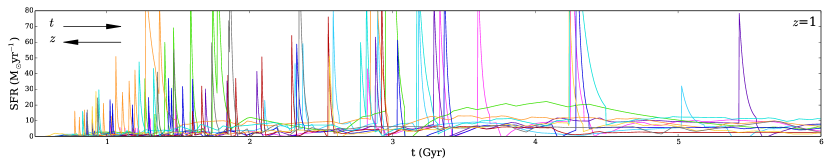
Figure 1: Examples of 10 SFHs of simulated galaxies extracted from the galform SAM.

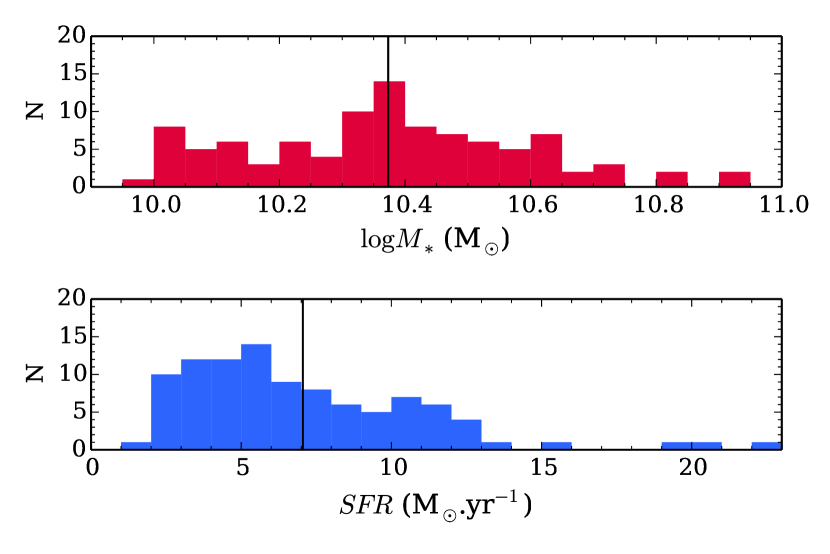
Figure 2: Distribution of $M_{*}$ and SFR associated with the galform SFHs. The black lines show the mean value of the distributions.

2.2 Simulations of UV to submm SEDs

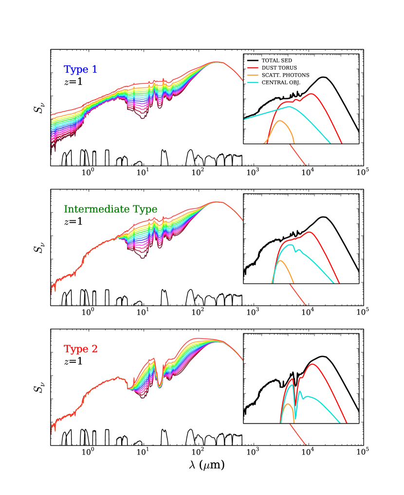
Figure 3: SEDs generated by GIGALE using a particular SFH extracted from galform and adding on that different AGN templates with different normalizations relative to the galaxy light. Each panel corresponds to one of the three Fritz et al. (2006) templates presented in Table LABEL:mockparam: the upper panel is for Type 1 AGN, the middle panel is for the Intermediate AGN type, and the lower panel is for Type 2 AGN. SEDs are color-coded according to the contribution of the AGN to the total IR luminosity. The black solid lines at the bottom of each panel are the broad-band filters of Table LABEL:filt, within which the model SEDs are integrated to generated mock photometric catalogues. The inset plots show the contribution of the three AGN components to the total SED for $frac_{AGN}$=40%. Red is for the dust torus emission, orange is the scattering component, and cyan the direct emission from the central AGN.

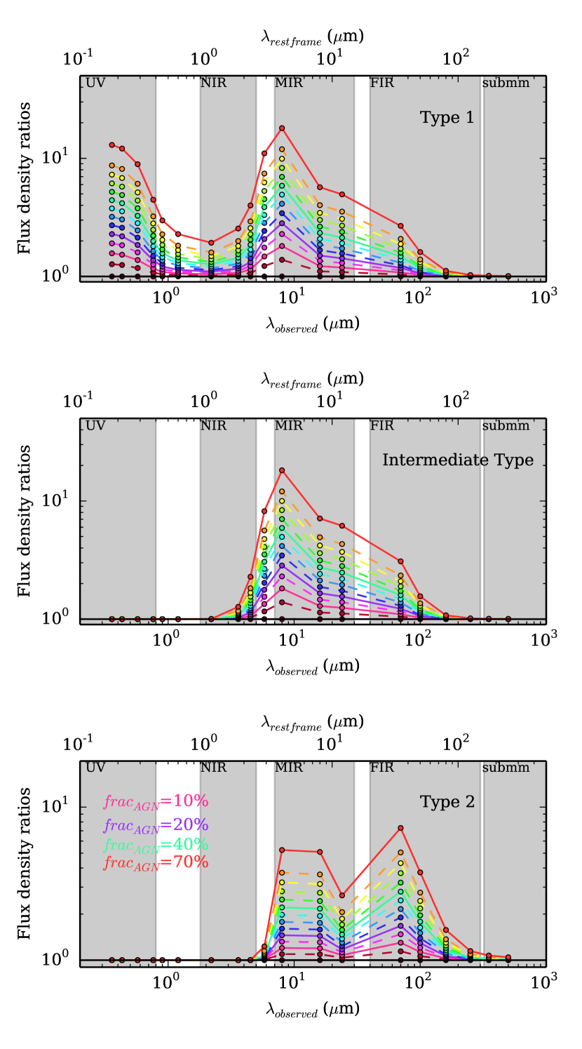
Figure 4: The SEDs of Figure 3 normalized to the SED with no AGN emission, i.e. $frac_{AGN}=0$. The three panels correspond to one of the Fritz et al. (2006) templates presented in Table LABEL:mockparam: upper panel is for Type 1 AGN, the middle panel corresponds to the intermediate AGN type, and the lower panel is for the Type 2 AGN. The grey regions indicated different rest frame spectral domains from UV to sub-mm. Normalized SEDs are color-coded according to the $frac_{AGN}$ parameter. Solid colored lines indicate specific SEDs, i.e. where $frac_{AGN}$=10% (pink), 20% (purple), 40% (green), and 70% (red).

CIGALE is a package that has two different and independent functions: an SED modeling function (Boquien et al., in prep) and an SED fitting function (Burgarella et al., in prep). The baseline functions of CIGALE are presented in Noll et al. (2009). Based on the same general principles as the original version of CIGALE, this entirely new version has been designed for a broader set of scientific applications and better performance. The latest version of the modeling function of CIGALE is briefly described in this section.

The SED modeling function of CIGALE allows the construction of galaxy SEDs from the UV to the submm by assuming a stellar population library and star-formation histories provided by the user. CIGALE builds the SED taking into account energy balance, i.e., the energy absorbed by dust in UV-optical is reemitted in the IR.

In CIGALE, the SFH can be handled in two different ways. The first, is to model it using simple analytic functions (e.g. exponential forms, delayed SFHs, etc). The second is to provide more complex (non-analytic) SFHs (e.g., Boquien et al. 2014), such as those provided by the galform SAM. The stellar population models of either Maraston (2005) or Bruzual & Charlot (2003) are convolved with the adopted SFH to produce stellar SEDs, which are then attenuated by dust. The energy absorbed by the dust is reemitted in the IR using a choice of different dust templates (Dale & Helou 2002; Dale et al. 2014; Draine & Li 2007; Casey 2012).

CIGALE also allows the emission from AGN to be added to the stellar SED. The AGN templates from the library of Fritz et al. (2006) are adopted. These SEDs consist of two components. The first one is the isotropic emission of the central source, which is assumed to be point-like. This emission is a composition of power laws with variable indices in the wavelength range of 0.001-20 $\mu$m. The second component of the Fritz et al. (2006) models is radiation from dust with a toroidal geometry in the vicinity of the central engine. Part of the direct emission of the AGN is either absorbed by the toroidal obscurer and re-emitted at longer wavelength (1-1000 $\mu$m) or scattered by the same medium. Dust can be optically thick to its own radiation, thus requiring the numerical resolution of the radiative transfer problem. In Fritz et al. (2006) models, the conservation of energy is always verified within 1% for typical solutions, and up to 10% in the case of very high optical depth and non-constant dust density. The choice of adding the Fritz et al. (2006) library into CIGALE is driven by the energy balance handling of the two components, which also matches the energy conservation philosophy of CIGALE. Furthermore, this library has been tested in numerous studies of the literature (e.g., Fritz et al. 2006; Hatziminaoglou et al. 2008, 2010; Feltre et al. 2012).

The relative normalization of these AGN components to the host galaxy SED is handled through a parameter which is the fraction of the total IR luminosity due to the AGN so that

$$L_{IR}^{AGN}=frac_{AGN}\times L_{IR}^{TOT},$$ (1)

where $L_{IR}^{AGN}$ is the AGN IR luminosity, $frac_{AGN}$ is the contribution of the AGN to the total IR luminosity ($L_{IR}^{TOT}$), i.e. $L_{IR}^{starburst}+L_{IR}^{AGN}$. Thus, estimating $L_{IR}^{AGN}$ depends on the constraints on $frac_{AGN}$.

For each SFH provided by galform, we compute a host galaxy SED using the Maraston (2005) stellar population models and assuming the Calzetti et al. (2000) extinction law. The amount of reddening, $E(B-V)_{*}$, is chosen to be 0.2, motived by observational studies of AGN host galaxies (Kauffmann et al. 2003b; Hainline et al. 2012). The energy absorbed in UV-Opt-NIR is re-injected in IR, providing the normalization of the Draine & Li (2007) models in order to maintain the energy balance of the SED. The template is chosen following the results of Magdis et al. (2012) who fit high-$z$ galaxies with the Draine & Li (2007) models. The parameters used to model the galaxies are presented in Table LABEL:mockparam.

We select three AGN model templates from the Fritz et al. (2006) library to be added to the galaxy SEDs. These include a Type 1 AGN (i.e. unobscured), a Type 2 AGN (i.e. obscured) and a template that lies in-between the first two and is referred to as intermediate type. The latter model displays a power-law spectral shape in the mid-IR without strong UV/optical emission. Previous studies indicate that such an intermediate template is indeed necessary to represent the diversity of the observed SEDs of AGN (Hatziminaoglou et al. 2008, 2009; Feltre et al. 2012). The Fritz et al. (2006) model parameters for the three templates are presented in Table LABEL:mockparam. The parameters for the Type 1 and Type 2 AGN templates are representative of local unobscured and obscured AGN, respectively (Fritz et al. 2006). For the intermediate AGN type we adopt one of the Fritz et al. (2006) models with low equatorial optical depth (Hatziminaoglou et al. 2008, 2009; Feltre et al. 2012, Buat et al., in prep). The three AGN templates adopted in this paper are the minimum required to represent the variety of the broad-band AGN SEDs. There are strong degeneracies among different parameters of the Fritz et al. (2006) library that cannot be broken by multiwavelength photometric data alone. Additional parameters combinations to those shown in Table LABEL:mockparam do not necessarily result in AGN broad-band SEDs that are distinctively different from our Type 1, Type 2 and intermediate type models. In Figure 3, we show the SEDs corresponding to one of the SFHs presented in Figure 1.

The modeled SEDs are integrated within the broad band filters of Table LABEL:filt to produce mock photometric catalogues. These will be used in the next section to assess the reliability of AGN/galaxy decomposition using photometric data and quantify the level of accuracy at which physical parameters of the underlying galaxy can be derived. Random noise is added to the fluxes of each source assuming Gaussian errors with standard deviation 10% of the flux in a given waveband. We associate a photometric error of 15% with all the flux densities. The broad-band filters of Table LABEL:filt sample a wide range of wavelengths, as shown on Figure 3. In order to quantify the level of AGN contribution in each of these filters, we show in Figure 4 the flux density ratios of the SEDs that include an AGN component relative to those that do not ($frac_{AGN}=0$). A Type 1 AGN with a $frac_{AGN}=10\%$ will have an AGN emission higher by a factor of 2 in the UV and MIR rest frame compared to the same SED without an AGN component. In UV rest frame, a fraction $frac_{AGN}=40\%$ is sufficient to dominate the emission, with an AGN contribution four times higher than the young stellar population emission. In MIR rest frame, the AGN emission is dominant for $frac_{AGN}>$20% with an emission three times higher than the stellar emission. The UV and the MIR are thus key domains to perform AGN/galaxy decomposition in the case of a Type 1 AGN SED as also shown in previous work (e.g., Weedman et al. 2004; Wu et al. 2009). The AGN emission of the intermediate type is visible in the MIR domains, especially at 4 $\mu$m  rest frame, where it is brighter than the host galaxy by a factor of 2 for a fraction of 10%. For the Type 2 AGN, it is clear that the emission of the AGN cannot be detected below 2 $\mu$m  rest frame. In this model, the torus is optically thick and the emission from the inner, hotter part of the torus, emitting at shorter wavelength is completely absorbed. In FIR rest frame, the emission of the AGN contributing to 70% of the total $L_{IR}$ will dominate the emission of the host galaxy by a factor of 7. Given the ratio between the AGN emission and the host galaxy emission (Figure 4), two bands seem to be the key to constrain the Type 2 AGN emission, the 3-10 $\mu$m rest frame and the 30-40 $\mu$m rest frame as already noticed in previous works (e.g., Laurent et al. 2000). However, we note that dust emission templates are not well constrained in the 30-40 $\mu$m range (Ciesla et al. 2014) and thus improving them can help disentangling the AGN contribution in the FIR.

Table 1: Galaxy and AGN parameters adopted to generate mock galaxy SEDs.

Parameter	Value	Description
Dust attenuation
$E(B-V)_{*}$	0.2
Dust template: Draine & Li (2007)
$q_{PAH}$ (%)	3.19	Mass fraction of PAH to the total dust mass.
$U_{min}$	8.0	Min. intensity of the interstellar radiation field.
$U_{max}$	$10^{6}$	Max. intensity of the interstellar radiation field.
$\gamma$ (%)	2	Relative contribution between dust heated in photodissociation
		regions, and dust heated by diffuse stellar population.
AGN emission
$R_{max}/R_{min}$	60	Ratio between outer and inner radius of the torus.
$\tau_{9.7}$	1.0 (for int. type)	Optical depth at 9.7 $\mu$m.
	6.0 (for Type 1 & Type 2)
$\beta$	-0.5	Linked to the radial dust distribution in the torus.
$\gamma$	0.0	Linked to the angular dust distribution in the torus.
$\psi$	0.001 (for int. type & Type 2)	Angle with line of sight.
	89.9 (for Type 1)
$\theta$	100	Angular opening angle of the torus.
$frac_{AGN}$	0., 0.05, 0.1, 0.15, 0.2, 0.25, 0.3,	Contribution of the AGN to the total $L_{IR}$.
	0.35, 0.4, 0.45, 0.5, 0.55, 0.6, 0.7

Table 2: Broad-band filter-set used in this paper.

Telescope/Camera	Filter Name	$\lambda_{mean}$( $\mu$m)
MOSAIC	U	0.358
HST	ACS435	0.431
	ACS606	0.573
	ACS775	0.762
	ACS850	0.9
Subaru/MOIRCS	J	1.2
CFHT/WIRCam	Ks	2.2
Spitzer	IRAC1	3.6
	IRAC2	4.5
	IRAC3	5.8
	IRAC4	8
	IRS16	16
	MIPS1	24
	MIPS2	70
Herschel	PACS green	100
	PACS red	160
	PSW	250
	PMW	350
	PLW	500

3 Recovering the mock galaxy properties

The SED fitting functions of CIGALE are applied to the mock photometric galaxy catalogue of the previous section to separate the stellar emission from the AGN component and investigate how accurately stellar masses and star-formation rates can be determined for galaxies that host an AGN.

To perform the SED fitting analysis, CIGALE first builds models corresponding to a range of input parameters for both the stellar and AGN components. The adopted parameters used in the fitting procedure are presented in Table LABEL:fitparam. The ones related to the galaxy host emission templates are selected based on the experience gained from galaxy SED modeling at intermediate and high redshift using CIGALE (e.g., Giovannoli et al. 2011; Buat et al. 2012; Burgarella et al. 2013; Buat et al. 2014).

For the building of a galaxy template SED, it is first necessary to make some assumptions about the star-formation history, which will be convolved with the stellar libraries to yield galaxy SEDs. The SFH of real galaxies are expected to be highly stochastic. It is therefore impractical and probably meaningless to assume complex SFHs like those shown in Figure 1, when fitting multiwavelength photometric data. It is common practice instead, to assume simple functional forms, such as an exponentially decreasing SFR (1$\tau$-dec, e.g., Ilbert et al. 2013; Muzzin et al. 2013), an exponentially increasing SFR (1-exp-ris, e.g., Pforr et al. 2012; Reddy et al. 2012), two exponential decreasing SFR laws with different e-folding times (2$\tau$-dec, e.g., Papovich et al. 2001; Borch et al. 2006; Gawiser et al. 2007; Lee et al. 2009), a delayed SFR (e.g., Lee et al. 2010, 2011; Schaerer et al. 2013), or a lognormal SFH (Gladders et al. 2013). We consider in this work the 1$\tau$-dec, the 2$\tau$-dec, and the delayed models. First tests made with CIGALE on the lognormal SFH show that the parameters associated are not constrained by broad band photometry. However, as demonstrated in Figure 2 of Gladders et al. (2013), only specific combinations of the parameters of this SFH lead to a non null instantaneous SFR at the age of the galaxy. Thus, we do not consider here the lognormal SFH as it provides problematic SFRs. Furthermore, since the 1-exp-ris model is recommended to only model the SFH of galaxies at $z>$2 (e.g., Maraston et al. 2010; Papovich et al. 2011; Pforr et al. 2012; Reddy et al. 2012), we do not test it in this work.

The 1$\tau$-dec is represented by the following equation:

$$SFR(t)\propto exp(-t/\tau_{1})$$ (2)

where $t$ is the time and $\tau_{1}$ the e-folding time of the old stellar population. The 2$\tau$-dec is obtained adding a late burst to the 1$\tau$-dec SFH, and thus modeled as:

$$SFR(t)=\begin{cases}\exp{-t/\tau_{1}}&\text{if }t<t_{1}-t_{2}\\ \exp{-t/\tau_{1}}+k\times\exp{-t/\tau_{2}}&\text{if }t\geq t_{1}-t_{2}\end{cases}$$ (3)

where $\tau_{2}$ is the e-folding time of the young stellar population, and $k$ the amplitude of the second exponential which depends on the burst strength parameter $f_{ySP}$. Finally, the delayed SFH is defined as:

$$SFR(t)\propto t\,exp(-t/\tau_{1}).$$ (4)

We assume a Salpeter IMF and the stellar population models of Maraston (2005). The metallicity is fixed to the solar one, 0.02. Dust extinction is modeled assuming the Calzetti et al. (2000) law with $E(B-V)_{*}$ in the range of value shown in Table LABEL:fitparam. We also assume that old stars have lower extinction compared to young stellar populations by a fixed factor, $f_{att}=0.44$ (Calzetti et al. 2000). The UV/optical stellar emission absorbed by dust is remitted in the IR assuming the Dale et al. (2014) templates. We emphasize that this is different from the Draine & Li (2007) libraries used to generate the mock photometric catalogue (see Section 2 and Table LABEL:mockparam). This reduces the impact on the results of using the same assumptions/templates to generate and to fit the photometry of simulated extragalactic sources.

AGN templates are also included in the fitting procedure. In Appendix A, we demonstrate that in the case of AGN hosts this is essential to minimize biases in stellar mass and SFR estimates related to contamination of the stellar light by AGN emission. Ignoring this effect results in an over-estimation of the stellar mass by up to 150% and the SFR by up to 300% depending on the spectral type and the strength of the AGN component. The parameters used to fit the AGN component are chosen based on the results of Fritz et al. (2006). However, we decide to fix the value of $\beta$, $\gamma$, and $\theta$, that parametrized the density distribution of the dust within the torus, with typical values found by Fritz et al. (2006) to limit the number of models. Indeed, allowing for different values of these parameters would result in degenerated model templates.

Although the AGN parameters used to create the mock SEDs are not used in the fitting part of this work, we recognize that there could be potential problems with using the same template library to generate mock photometric data and then fit them. As a test, we have created the mock galaxies with observed AGN templates and fit them with the Fritz et al. (2006) models, the results are discussed in Section 3.4. We find that our results and conclusions are robust to the set of templates used to model/fit the AGN component of the SED.

The modeled SEDs are integrated into the selected set of filters, and these modeled flux densities are then compared to the ones of the input catalogue of galaxies. For each galaxy in the mock photometric catalogue, and for each set of model parameters, the $\chi^{2}$ is computed. The code then builds the probability distribution function (PDF) of the derived parameters of interest (e.g. stellar mass, SFR, $frac_{AGN}$) based on the $\chi^{2}$ value of the fits. The output value of a parameter is the mean value of the PDF, and the associated error is the standard deviation determined from the PDF. We refer the reader to Noll et al. (2009) for more information on the Bayesian-like analysis performed by CIGALE.

To avoid any bias that could rise from the fact that we use the same tool to create and analyze the mock SEDs, we take the following precautions:

• The flux densities of the mock SEDs are perturbed by adding a noise randomly taken in a Gaussian distribution with a standard deviation of 0.1.

• We use simple analytic SFHs in the SED fitting procedure in order to reproduce galform SFHs.

• Although the mock galaxies dust emission is modeled with the Draine & Li (2007) library, we use the Dale et al. (2014) templates in the SED fitting.

• Even though we also use the Fritz et al. (2006) library to perform the fitting, we prevent CIGALE to use the templates used in the building of the mocks catalogues. We did not use a different AGN library for our fitting procedure for two reasons. The first one is that we are limited by the AGN models available in CIGALE. The second one is that it has been shown in Feltre et al. (2012) that the smooth torus library of Fritz et al. (2006) is highly degenerated with the clumpy torus library of Nenkova et al. (2008). Thus using for instance this very different library will not affect our results.

Table 3: Parameter ranges used in the blind fitting procedure.

Parameter	Symbol	Values
Star Formation History
Metallicity	$Z$	0.02
IMF		Salpeter
Double exponentially decreasing
$\tau$ of old stellar population models (Gyr)	$\tau_{1}$	1, 3, 5
Age of old stellar population models (Gyr)	$t_{1}$	1, 2, 3, 4, 5
$\tau$ of young stellar population models (Gyr)	$\tau_{2}$	10.
Age of young stellar population models (Gyr)	$t_{2}$	0.01, 0.03, 0.1, 0.3
Mass fraction of young stellar population	$f_{ySP}$	0.001, 0.01, 0.1, 0.2
Single exponentially decreasing
$\tau$ of stellar population models (Gyr)	$\tau$	0.5, 1, 3, 5, 10
Age of stellar population models (Gyr)	$t$	1, 2, 3, 4, 5
Delayed SFH
$\tau$ of stellar population models (Gyr)	$\tau$	0.5, 1, 3, 5, 10
Age (Gyr)	$t$	4, 5, 5.5
Dust Attenuation
Colour excess of stellar continuum light for the young population	$E(B-V)_{*}$	0.05, 0.1,0.15, 0.2, 0.25, 0.3,0.35, 0.4, 0.5,0.6
$E(B-V)_{*}$ reduction factor between old and young populations	$f_{att}$	0.44
Dust template
IR power-law slope	$\alpha$	1.5, 2, 2.5
AGN emission
Ratio of dust torus radii	$R_{max}/R_{min}$	30, 100
	$\tau_{9.7}$	0.3, 3.0, 6.0, 10.0
	$\beta$	-0.5
	$\gamma$	0.00
	$\psi$	0.001, 50.100, 89.990
Opening angle of the torus	$\theta$	100
Fraction of $L_{IR}$ due to the AGN	$frac_{AGN}$	-0.2, -0.15, -0.1, -0.05, 0.0, 0.05, 0.1, 0.15, 0.2
		0.25, 0.3, 0.4, 0.5, 0.6, 0.7, 0.8

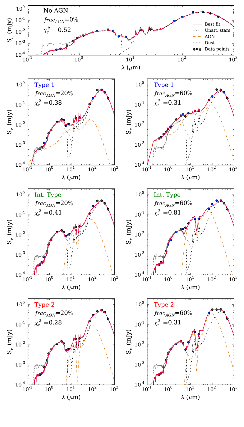
Figure 5: Examples of fits for mock galaxies associated with one of the SFHs shown is Figure 1. Blue points are the flux densities of the mock galaxies, the red lines are the best fits obtained by CIGALE. In addition, we show the unattenuated stellar emission in black dotted line, the dust emission in black dashed-dotted line, and the total emission from the AGN in orange dashed line. The associated reduced $\chi^{2}$ are provided. The single top panel shows the best fit in the absence of AGN emission. The two upper panels show the best fit for Type 1 with a fraction of 20% (left) and a fraction of 60% (right), the middle ones for the intermediate type, and the bottom panels for the Type 2 AGN.

We present in Figure 5 examples of fits of the mock galaxies corresponding to the galform SFH presented in Figure 1, and assuming a double exponentially decreasing SFH. In Type 1 and intermediate type AGNs, the fits are good but we note some difficulties in reproducing measurement near the IR peak. This disagreement is attributed to compatibility problems between Dale et al. (2014) and Draine & Li (2007) dust emission libraries in this range (Ciesla et al. 2014) that have no impact on the results of this study. For the intermediate type AGN, Figure 5 shows that the code uses a model with a strong silicate absorption at 9.7 $\mu$m. However, as shown in Figure 3 (middle panel), the input AGN model used for the intermediate type does not show any silicate absorption. Thus, despite the availability of models with low values of $\tau_{9.7}$ in the fitting procedure, the code does not reproduce the absence of silicate absorption of the input SED. Although these points have no impact on the result of this study, they give a glimpse on possible problems to constrain AGN templates with broad-band photometry.

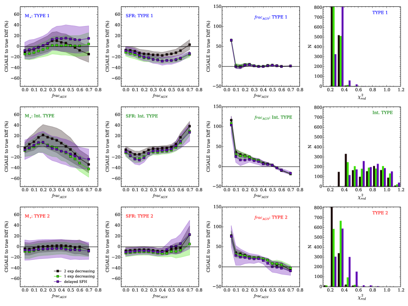
Figure 6: Fractional difference between parameters derived from CIGALE and the simulated ones as a function of $frac_{AGN}$, i.e. the contribution of the AGN light to the overall IR luminosity. The first column of panels plots the fractional difference in stellar mass estimates. The second column is for SFR estimates and the third column corresponds to $frac_{AGN}$. The fourth column of panels shows the distribution of $\chi_{red}^{2}$. Each row corresponds to a set of simulation that assume different input SEDs for the AGN component. From top to bottom, we present results for Type 1 AGN, intermediate type and Type 2 AGN. Different colors in each panel correspond to different functional forms for the SFH. Black is for the 2$\tau$-dec model, green corresponds to the 1$\tau$-dec model, and purple marks the delayed SFH. Dots represent the mean value of the fractional difference at each input $frac_{AGN}$, the shaded regions show the one $\sigma$ scatter.

The estimates of the $M_{*}$, SFR, and $frac_{AGN}$ as a function of the contribution of the AGN are presented in Figure 6 for the three different assumptions made on the SFH, as well as the $\chi^{2}_{red}$ distribution for each case. We discuss these results in the absence of AGN in Section 3.1, and the impact of the AGN contribution in Section 3.2.

3.1 Determining stellar masses and star formation rates in simulated galaxies without AGN component

Table 4: Fractional differences between the derived $M_{*}$ and SFR and the input ones for the mock galaxies with $frac_{AGN}=0$ (no AGN contribution).

SFH model	$M_{*}$		SFR
	mean (%)	$\sigma$ (%)	mean (%)	$\sigma$ (%)
1$\tau$-dec	-10.0	11.5	-11.4	7.0
2$\tau$-dec	-5.2	10.2	-6.6	6.2
delayed	-6.5	17.6	-9.1	7.4

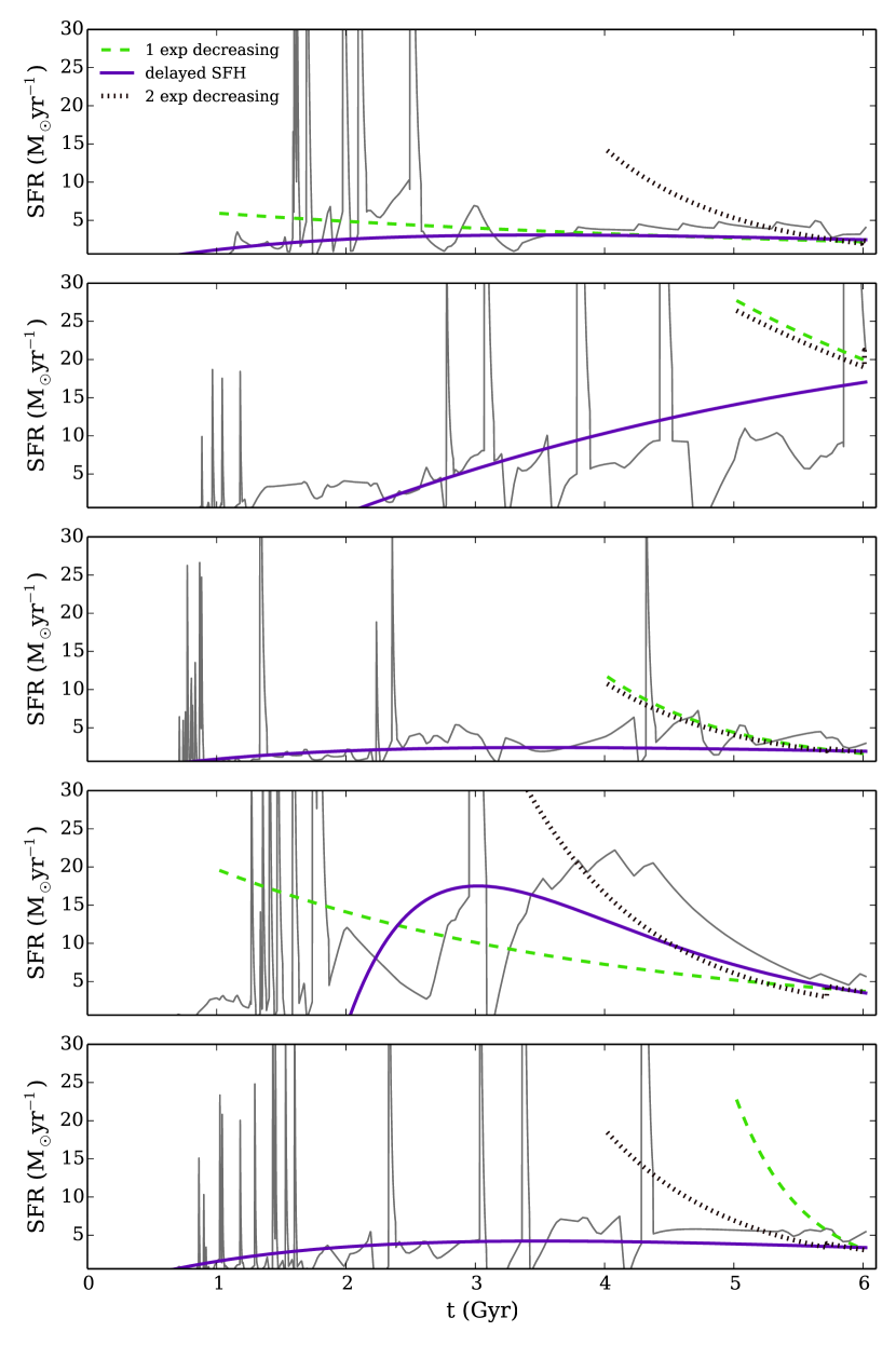
Figure 7: Comparison between five SFHs from galform and the corresponding best-fit output SFHs obtained by CIGALE. The green dashed-line is for the 1$\tau$-dec model, the purple solid-line corresponds to the delayed SFH, and the black dotted-line to the 2$\tau$-dec model.

We first explore fractional differences between the derived and input stellar masses and SFRs for mock galaxies without any AGN component included in their SEDs, i.e. the case $frac_{AGN}=0$ in Figure 6. Both parameters depend on the adopted SFH used to fit the mock galaxy multi-waveband photometry. Different functional forms for the SFH are expected to induce systematic variations in both $M_{*}$ and SFR determinations (Bell et al. 2003; Lee et al. 2009; Maraston et al. 2010; Pforr et al. 2012). Table LABEL:offsets provides the fractional systematic offsets for the different SFH assumptions used in our analysis to fit the mock galaxy photometry. The model that provides on average the best agreement between the output and input $M_{*}$ and SFRs is the 2$\tau$-dec.

In order to compare the output parameters linked to SFH, we show on Figure 7 five galform SFHs as well as the associated SFHs obtained from the best fit of the SED fitting procedure. galform SFHs are complex and analytical SFHs cannot reproduce the numerous star formation bursts. However, as the integral of the SFH provide the stellar mass of the galaxy, it is clear that, in order to recover the stellar mass, the best 1$\tau$-dec and 2$\tau$-dec models use a very small, unrealistic age. Indeed, if we fix the age of the galaxy, contrary to what is usually done in the literature when using these assumptions, by providing a smaller age range, between 4 and 5.5 Gyr for our samples as galaxies are at $z$=1, then these two models overestimate $M_{*}$ by 15 and 19%, respectively. From the three SFHs models used in this work, the delayed SFH better reproduces the global envelop of the galform SFH. As a result this functional form yields stellar masses in reasonable agreement with the input ones and, at the same time, a galaxy formation age close to the simulated one. This is consistent with the mean SFHs of Illustris presented in Sparre et al. (2014). Indeed, the mean and median SFHs of Illustris sources have shapes that can be typically modeled with a delayed SFH. This result obtained from Semi-Analytical Models of galaxy evolution seems to be in agreement with the conclusions of Boselli et al. (2001) based on observations of local galaxies. We thus conclude that a delayed SFH seems to be a more realistic assumption on the SFH of galaxies.

Several published works have studied the ability of SED fitting techniques to retrieve the stellar mass of galaxies. They were based on mock catalogues, on SAMs, or on hydrodynamical codes, and some of them made use of the IR domain (Wuyts et al. 2009; Lee et al. 2009; Pforr et al. 2012; Pacifici et al. 2012; Mitchell et al. 2013; Buat et al. 2014). Also using galform SFHs, Mitchell et al. (2013) showed that a single exponentially decreasing SFH provides a good estimation of $M_{*}$ with a small offset of -0.03 dex. Using CIGALE, (Buat et al. 2014) found that the output stellar mass is systematically lower by 0.07 dex compared to the true one. Despite the different methods used in these works, our results are in good agreement as we find an underestimation of the stellar mass of $\sim$7% averaged over the three types of SFH.

Small differences are also found in the derivation of the SFR from the different SFH assumptions, but they globally slightly underestimate the SFR with offsets between 6.6 and 11.4% (Table LABEL:offsets). These relatively good estimations ($<$12%) obtained with the SFR are in perfect agreement with the results of Buat et al. (2014) who found that the SFR is robustly estimated, with systematic differences lower than 10%, whatever the chosen SFH model as long as one IR data is available.

Another parameter which is known to be directly linked to the estimation of the stellar masses and SFR is the amount of attenuation, quantified in this work by $E(B-V)_{*}$. The link between the attenuation and the stellar mass is however indirect. Without a strong constraint on the dust attenuation, a degeneracy between the age of the old stellar population (which is directly linked to the stellar mass) and the attenuation appears (Pforr et al. 2012; Conroy 2013; Buat et al. 2014). We explore this bias by generating mock galaxy photometry by varying the $E(B-V)_{*}$ input value and fixing $frac_{AGN}$=0. The resulting mocks catalogues are fit with a 2$\tau$-dec SFH model. The systematic offset of the derived $M_{*}$ increases by a factor of two between $E(B-V)_{*}=0.05$ and $E(B-V)_{*}=0.7$. The underestimation on the SFR varies from -15% to -6% for $E(B-V)_{*}=0.05$ ($A_{V}$=0.2 mag) to $E(B-V)_{*}=0.5$ ($A_{V}$=2 mag). Furthermore, if we use, in the mock catalogues, a host galaxy SED with a completely obscured star formation, then the contribution of the AGN to the total IR luminosity is still recovered for high fractions, but the offset between 15$\%$ and 30$\%$ is larger by a factor of $\sim$2. Thus the level of stellar light attenuation also plays a role in recovering the stellar mass and SFR of galaxies, as already shown in previous studies (e.g., Wuyts et al. 2009; Mitchell et al. 2013; Buat et al. 2014).

In conclusion, the 2$\tau$-dec model provides the best estimates of $M_{*}$ and SFR of the simulated galaxies, in the expense of unrealistic galaxy ages. The delayed SFH recovers the stellar mass with a mean offset of $\sim$6.5%, and a mean offset on the SFR of $\sim$9%, but better reproduces the true SFH of the galaxies. We use the results obtained in absence of AGN emission as references to analyze the AGN impact on the estimation of $M_{*}$ and SFR.

3.2 Determining stellar masses and star formation rates in AGN host galaxies

As shown in Figure 4, depending on its intensity, the AGN emission contaminates large parts of the SED especially the key domains used to retrieve the stellar mass and the SFR of the underlying galaxy. In this Section, we discuss the ability of broad band SED fitting to constrain this contamination, decompose the AGN from the host galaxy light, determine stellar masses and SFR of AGN hosts. The results are presented in Figure 6 for the three AGN types considered in this work, where we show the mean fractional difference for each parameter as a function of the input power of the AGN (points), as well the 1-$\sigma$ scatter (shaded regions).

3.2.1 Constraining the AGN contribution

First we explore the ability of CIGALE to constrain the fractional contribution of AGN emission to the total IR luminosity, i.e. the $frac_{AGN}$ parameter. The set of panels in the third column of Figure 6 presents the relative difference between the output and input $frac_{AGN}$ averaged over the 100 galform  SFHs, for the different assumptions of SFHs. The AGN contribution is almost always overestimated for all three types, except for high fraction values ($frac_{AGN}>$50%) for the intermediate type and Type 2 AGNs, where it is underestimated. Independent from the input AGN SED shape (Type 1, intermediate type, or Type 2), below $frac_{AGN}$=10%, there is a large overestimation of the AGN contribution, that can reach up to $\sim$120%. One explanation could be the well-known effect of the use of PDF analysis in retrieving parameters. For the lowest value of the parameter, the PDF will be truncated, and thus taking its mean value will slightly shift the output value of the parameter toward a larger value, yielding to its overestimation, as explained in Noll et al. (2009) and Buat et al. (2012). However, to prevent this effect, we provide low negative $frac_{AGN}$ as well as input parameters. Without any impact on the results of the SED fitting and the estimates of $M_{*}$ and SFR, it allows a better estimate of very low $frac_{AGN}$ from the PDF analysis. Thus, the overestimation observed for very low fractions shows the difficulty CIGALE has to distinguish between a SED without any AGN contamination and an SED with a very low contribution of the AGN ($\sim$5%). We thus conclude that low AGN contributions are very difficult to constraint from broad band SED fitting with an overestimation up to a factor of 2 for $frac_{AGN}<$10%. At higher fractions, the overestimation depends on the type of AGN. A Type 1 contribution to the total $L_{IR}$ is well recovered with an offset smaller than 10% for fractions higher than 10%. In order to better understand this trend, we show in Figure 8 (left panel) the PDF for each $frac_{AGN}$ as seen from the top of it, for the SEDs associated to one SFH. We can see from Figure 8 that the shape and position of the PDF do not change when $frac_{AGN}$ increases. For the intermediate type and Type 2, an overestimation of 30-40% can be expected for $frac_{AGN}$ between 10 and 40%. Then the offset decreases at higher fractions. These effects are seen on Figure 8, the PDF is large for low values of $frac_{AGN}$ and shows a constant overestimation up to high values of $frac_{AGN}$, i.e. 60%.

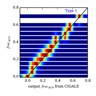
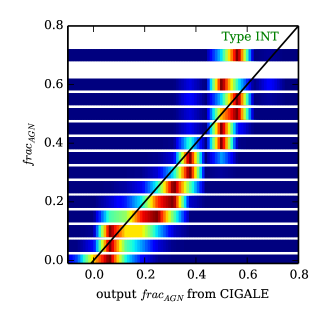
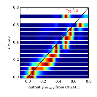
Figure 8: Probability distribution function for the $frac_{AGN}$ determination of a particular galform SFH. The vertical axis in all panels corresponds to different input $frac_{AGN}$. Each panel corresponds to a different AGN SED added to the stellar light: left is for the Type 1 AGN, the middle panel corresponds to the intermediate AGN type, and right panel plots the results for the Type 2 AGN. The color indicates the level of probability, blue being the lowest probability and red the highest. The black solid line is the one to one relationship.

3.2.2 Estimating the stellar mass

The panels in the first column of Figure 6 plot the fractional difference between the input stellar mass of AGN hosts and that inferred from the template fits to the mock photometry. This figure shows that the stellar masses of AGN hosts can be derived with systematic uncertainties smaller than 40% ($\Delta\log M_{*}<0.15$ dex), even in the case of Type 1 AGNs and up to $frac_{AGN}=0.7$. This underlines the importance of AGN/stellar light decomposition when fitting templates to multi-wavelength photometric data of AGN to derive properties of the underlying galaxy. If AGN templates were not included in the analysis the inferred stellar masses would be biased to high values by a factor as large as 2.5 (see Appendix A).

Careful inspection of Figure 6 also suggests that, in the case of Type 1 AGN, the uncertainties on the estimation of $M_{*}$ as a function of Type 1 AGN fraction seem to not depend on the assumption made on the SFH up to $frac_{AGN}=$0.4. The fractional difference shows a constant increase up to $frac_{AGN}<$0.4 and then reaches a plateau for higher fractions, except for the 2$\tau$-dec model for which the offset decreases. Indeed, as we can see from Figure 4 (upper panel), at an AGN fraction of 20%, the AGN emission is higher than the host emission by a factor of 2 in the end of the NIR domain. As NIR flux densities are known to be a proxy for the stellar mass as the emission is dominated by the old stellar population (e.g., Gavazzi et al. 1996), it is sensible to think that there is a link between the contribution of the AGN in NIR and the variations observed in Figure 6. To understand this trend, we see in Figure 9 (left panel) the PDF of the stellar mass for each $frac_{AGN}$ as seen from the top of it. The PDF is very broad and is skewed toward lower values of $M_{*}$ when the $frac_{AGN}$ increases. The variation of the fractional difference in Type 1 AGNs depends on the contribution of the AGN to the total $L_{IR}$. A very weak effect can be attributed to the assumption made on the SFH but the 1$\sigma$ scatter of each of them are overlapping showing that this effect is marginal.

A systematic effect is seen in the intermediate AGN type (Figure 6, first column, middle panel). The offset on the stellar mass slightly increases with the contribution of AGN up to $frac_{AGN}\sim$20–30% and then decreases. This threshold of $frac_{AGN}\sim$20–30% corresponds to the point where the $frac_{AGN}$ starts to be relatively well constrained, even if it is still overestimated. We note that the delayed SFH appears relatively less affected showing weaker amplitude of variations with $frac_{AGN}$. Given the same pattern observed for three SFHs considered, the variation seen here is mostly due to the AGN emission.

For Type 2 sources, the AGN emission has no influence on the derivation of $M_{*}$ whatever the SFH chosen. This is likely due to the high obscuration of the light emitted from the accreting supermassive black hole, affecting only slightly the observed rest-frame NIR flux of the galaxy. Indeed, it is clear from Figure 4 that the NIR rest frame domain is not contaminated by the AGN emission. The $M_{*}$ PDF is relatively narrow and shows the offset discussed in Section 3.1 (Figure 9, right panel).

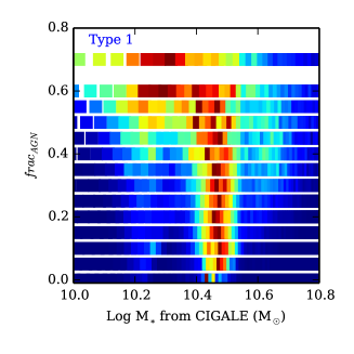
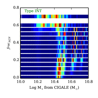
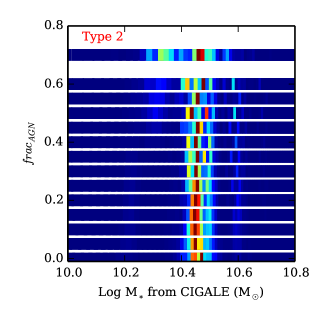
Figure 9: Probability distribution function for the $M_{*}$ determination of a particular galform SFH. The vertical axis in all panels corresponds to different input $frac_{AGN}$. Each panel corresponds to a different AGN SED added to the stellar light: left is for the Type 1 AGN, the middle panel corresponds to the intermediate AGN type, and right panel plots the results for the Type 2 AGN. The color indicates the level of probability, blue being the lowest probability and red the highest. The true $\log M_{*}$ for the particular simulated galaxy is 10.39 in solar units.

3.2.3 Estimating the star formation rate

For all three types of AGN considered in this work, the variation of the SFR estimation as a function of AGN strength is the same for the 1$\tau$-dec, 2$\tau$-dec, and delayed SFH. This implies that these variations are entirely due to the AGN emission. For Type 1 AGNs, the underestimation of the SFR increases with $frac_{AGN}$ up to 50%. Indeed, as shown on Figure 4, the UV becomes totally dominated by the AGN emission very quickly. However, the FIR is not much affected by the AGN emission which only dominates the 30 $\mu$m rest frame emission by a factor of 3 for the highest $frac_{AGN}$. This allows us to still constrain the attenuation and thus the SFR, even when there is an AGN contamination and estimate the SFR with a maximum offset of 30%. The example of Figure 10 (left panel) shows that the PDF is close to the true value, but in this case, a secondary peak arises for AGN fractions higher than 35%, yielding to the under-estimation.

In the case of the intermediate AGN type and for input AGN fractions of $frac_{AGN}=$10% the host galaxy SFR is underestimated by a factor of 20-30%. This is likely related to the overestimation of the AGN contribution to the FIR luminosity (see Figure 6 third column, middle panel). This results in an underestimation of the host galaxy emission in the MIR-FIR domain, and thus an underestimation of the SFR. However, for input $frac_{AGN}$ in the interval 25–50%, the AGN contribution to the FIR luminosity is better constrained. As a result the inferred SFR from the SED fit is also in better agreement with the input one. For input $frac_{AGN}\ga 50$% the opposite is happening. The AGN contribution to the FIR is underestimated and hence the host galaxy emission in the rest-frame MIR-FIR part of the SED is overestimated. The net effect is an overall overestimation of the SFR up to 40%. This behavior is also shown in Figure 10 (middle panel) where the peak of the PDF is slightly shifted toward lower values up to $frac_{AGN}$=30%, then lies on the right values up to $frac_{AGN}$=60% where the SFR starts to be overestimated for very high fractions.

For Type 2 AGNs, we find the same pattern as in the two previous cases. The 1$\tau$-dec, 2$\tau$-dec, and delayed SFH follow the same trend. The estimation of the SFR is quite insensitive to the AGN contribution with a very weak decreasing up to $frac_{AGN}$=40%. For higher fractions, the offset on the SFR measurement increases up to an over-estimation up to 20% for the 2$\tau$-dec and the delayed SFH models. A comparison between the SED with a AGN contribution of 40% and the SED of normal galaxy shows an emission three times higher for the AGN SED in the FIR domain, mandatory to have a good estimation of the SFR (Buat et al. 2014). The SFR PDF corresponding to the 2$\tau$-dec model (Figure 10, right panel) shows two peaks, one on the right value and one slightly overestimating the SFR. For high AGN fractions, a third peak arises overestimating even more the SFR and skewing the PDF toward higher values. However, this increase is weak for the 1$\tau$-dec SFH model yielding to overestimation of 5%–10% at $frac_{AGN}$=70%.

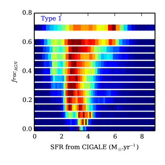
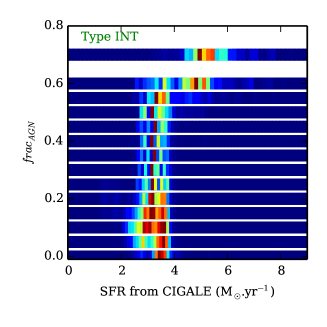
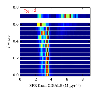
Figure 10: Probability distribution function for the SFR determination of a particular galform SFH. The vertical axis in all panels corresponds to different input $frac_{AGN}$. Each panel corresponds to a different AGN SED added to the stellar light: left is for the Type 1 AGN, the middle panel corresponds to the intermediate AGN type, and right panel plots the results for the Type 2 AGN. The color indicates the level of probability, blue being the lowest probability and red the highest. The true SFR for the particular simulated galaxy is 3.3 M_⊙.yr^-1.

3.3 Impact of the photometric coverage

The results presented in Section 3.1 and Section 3.2 have been tested in the ideal case where complete photometric coverage, from UV to submm rest frame, is available for each source. In this section, we study how the lack of photometric data at different spectral bands affects the determination of the stellar mass, the SFR, and the $frac_{AGN}$ parameter. As shown in Section 3.1, there is no perfect SFH assumption, we thus arbitrarily choose the 2$\tau$-dec SFH model. This choice does not affect the discussion because we are interested in deviations of the parameters inferred from spectral fits using incomplete broad-band coverage relative to the ideal case that all spectral bands listed in Table LABEL:filt are available. We run our SED fitting procedure using exactly the same parameters as in the previous sections. However, in successive runs, the input mock catalogues lack photometry in certain broad-band filters. We explore in particular how the results on stellar mass, SFR, and $frac_{AGN}$ change if we exclude in turn, the sub-mm rest frame ( Herschel/SPIRE 350 $\mu$m and 500 $\mu$m), the FIR rest frame (filters with $\lambda_{mean}\geq 24$ $\mu$m  in Table LABEL:filt), the mid-IR rest frame (filters with $\lambda_{mean}\geq 8$ $\mu$m in Table LABEL:filt), and the UV rest frame (filters with $\lambda_{mean}<0.762$ $\mu$m in Table LABEL:filt).

Figure 11 presents the results for each trial. The impact of the different spectral ranges in constraining the AGN contribution is shown in the third column of Figure 11. The lack of UV rest frame photometry has no impact in the determination of $frac_{AGN}$, even for Type 1 AGNs. This parameter is more sensitive to the availability of FIR and submm photometry. For all input AGN spectral types and for input $frac_{AGN}\ga 10-20\%$, the lack of IR and/or sub-mm data results in a systematic underestimation of inferred $frac_{AGN}$ up to typically 20-30% relative to the case of complete photometric coverage. Intermediate type and Type2 AGN show larger deviations compared to Type 1 AGNs. Interestingly, for input $frac_{AGN}\la 10-20\%$, the largest offset is found in the absence of submm data, showing the importance for these long wavelengths in constraining the emission from dust heated by young and evolved stellar populations. The exclusion of all photometric bands above 8 $\mu$m produces systematic offsets of up to 50% in the derived $frac_{AGN}$. This is expected because CIGALE is based on energy balance and therefore requires long wavelength data for optimum performance (Noll et al. 2009).

The first column of panels in Figure 11 shows changes in the determination of stellar mass for different set of photometric bands. The absence of FIR and/or submm has no significant impact on the derivation of the stellar mass for any of three AGN spectral types. The observed systematic variations with $frac_{AGN}$ are similar to the case of complete photometric band coverage. However, we note a small underestimation of $\sim$10% in $M_{*}$ for intermediate type with input $frac_{AGN}$ between 30 and 60%. The lack of UV photometry has no impact on the determination of $M_{*}$ for Type 2 AGN. This is because in this case there is no AGN emission to contaminate the UV–to–NIR bands. The absence of UV photometry however, does affect the $M_{*}$ estimates for Type 1 and intermediate type AGN. It leads to an underestimation of the stellar mass in Type 1 AGNs, and an overestimation for intermediate type AGN for input $frac_{AGN}=30-60\%$. This underlines the importance of the UV to recover the stellar mass for these types of AGNs. When no data longward of observed 8 $\mu$m  are available, the stellar mass is always moderately underestimated by up to 20-30%, relative to the case of full photometric band coverage. This is in agreement with Noll et al. (2009) who found an underestimation of 0.19 dex in the case of local normal (i.e. no AGN component) galaxies for the same combination of photometric data.

The panels in the second column of Figure 11 shows that the photometric coverage has an impact on the determination of SFR in AGN dominated galaxies. The strongest effects are observed in absence of data above observed 8 $\mu$m. This yields large systematic errors of 150-800% in SFR, depending on the level of input $frac_{AGN}$. This is in agreement with Noll et al. (2009) who also found an overestimation of the SFR by 0.83 dex for normal galaxies (i.e. no AGN component) for the same photometric data coverage. Smaller offsets in SFR estimates are found when the FIR, sub-mm and UV photometric bands are excluded. For Type 1 and Type 2 AGNs, the absence of any of these spectral domains leads to a systematic overestimation of 5–20%. In the case of intermediate type AGNs, the removal of the submm leads to variations in the estimation of the SFR up to $\sim$20%. The situation is worse when no FIR data is available, where the offset on the SFR increases rapidly with input $frac_{AGN}$ up to 35%. The absence of UV data for intermediate type AGNs has a peculiar effect as it starts to have an impact from $frac_{AGN}$=20%, where the SFR is underestimated up to $frac_{AGN}$=60%. In intermediate types, the AGN has no impact in the UV domain, as shown in Figure 3 and Figure 4. Removing this range forces CIGALE to rely on the FIR to estimate the SFR, which is contaminated by the AGN emission. It is therefore difficult to constrain the SFR of objects with AGN SED components similar to the intermediate type AGN considered in this work without any UV data.

Regarding constraints on the stellar mass in the case of SEDs without AGN contribution ($frac_{AGN}=0$), very small differences, less than a few percent, are observed when reducing the available photometric bands. This is expected since $M_{*}$ is mainly constrained from the NIR rest frame emission. The estimation of the SFR differs by up to $\sim$10% when we remove IR and UV data. This is to be expected since these spectral domains are important to constrain the SFR.

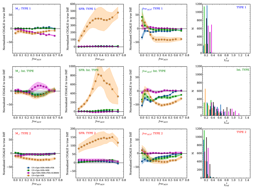
Figure 11: Evolution of the relative difference between output parameters from CIGALE and the true ones with the input fraction of AGN for the three types of AGN considered, normalized to the values obtained with a full photometric coverage. The blue relation corresponds to a photometric coverage containing no submm photometry. Green corresponds to the absence of FIR-submm data. Orange corresponds to the absence of IR data. Finally, the UV was removed for the magenta relation. $\chi^{2}_{red}$ distribution are shown for every run on the fourth column, we add the distribution corresponding to the total photometric coverage in black for comparison.

3.4 Impact of the AGN library

In order to focus our study on the biases that AGN emission has on the estimate on $M_{*}$ and SFR, we modeled the mock galaxies using templates from the Fritz et al. (2006) library, and used the same library to perform the SED fitting. Although we are cautious not to use the same AGN templates when simulating and fitting the mock galaxy photometry, it may be possible that the trends we observe are at least partially driven by degeneracies among the broad-band AGN SEDs of the Fritz et al. (2006) library. We explore this by using a different set of AGN templates to build the mock galaxy photometric catalogue. We select three SEDs presented by Lusso et al. (2013), derived by Silva et al. (2004), their Seyfert 1, their mildly obscured Seyfert 2 with $\log N_{H}$=21.5 $\rm cm^{-2}$, and their heavily obscured Seyfert 2 with $\log N_{H}$=24.5 $\rm cm^{-2}$. These templates bear similarities to the the Type 1, Intermediate type, and Type 2 Fritz et al. (2006) AGN templates defined in Table LABEL:mockparam. The approach described in Section 2.2 is followed to construct mock galaxy/AGN composite photometry, with the only difference that the three Lusso et al. (2013) templates above are used instead of the Fritz et al. (2006) ones. The SED fitting of the resulting mock galaxy catalogues follows the steps described in Section 2.2 (i.e. using Fritz et al. 2006, templates). Figure 12 presents in the same way as Figure 6 the results on stellar mass, SFR, and $frac_{AGN}$ for the 2$\tau$-dec SFH model. For these parameters the overall systematic trends in Figure 12 are similar to those observed in Figure 6 where the modeling of the mock galaxies is made with Fritz et al. (2006) models. We are therefore confident that our results are insensitive to the adopted AGN template library.

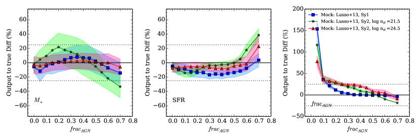
Figure 12: Comparison between the output values of $M_{*}$, SFR, and $frac_{AGN}$ and the true ones in the case where the AGN emission of the mock galaxies is modeled using Lusso et al. (2013) templates. The SED fitting is made using the 2$\tau$-dec SFH models, and the Fritz et al. (2006) models. The results for the Type 1 sample are in blue, for the intermediate type sample are in green, and for the Type 2 sample in red.

4 SFR–$M_{*}$ relation

As mentioned earlier, SED fitting is the most popular method to derive the physical properties of very large galaxy samples often produced by deep wide area extragalactic surveys. Recent studies of such large samples showed that the majority of star-forming galaxies are known to follow a SFR–$M_{*}$ correlation, called the main sequence (MS), and galaxies that lie above this sequence are experiencing a starburst event (Elbaz et al. 2011). In order to understand if the results discussed in this work could impact the shape of the MS, we show, in Figure 13, the mock galaxies of our samples in a SFR–$M_{*}$ plot. It is known that the main sequence predicted by models currently suffers normalization problems compared to the observed relation (e.g., Mitchell et al. 2014; Furlong et al. 2014). At $z$=1 the MS predicted by galform is about a factor of 2 lower than the observed MS (see Mitchell et al. 2014, for a complete discussion of this issue). The SFHs provided by galform are thus probably not a perfect representation of the real $z$=1 star forming galaxies, and it is unclear if it could affect our results. Indeed, all the models currently available suffer from the same issue. However, in this Section, we focus on the effect of the AGN emission and the use of SED fitting to retrieve the physical parameters of the galaxies on the MS.

As we discuss in Section 3.1 and Section 3.2, the choice of the SFH assumption has an impact of $M_{*}$ and SFR, and thus on the SFR–$M_{*}$ correlation, as also discussed in Buat et al. (2014). The stellar masses and SFR used in Figure 13 are those obtained from a 2$\tau$-dec SFH. The SFR–$M_{*}$ relation obtained from the Type 1 sample shows a small increase of the dispersion slightly shifted toward higher stellar masses, due to the offset on the stellar mass obtained for high fractions of AGN discussed in Section 3.1 (Figure 13, upper left panel). Thus, the increasing offset on the stellar mass estimation for Type 1 AGNs has a small impact of the SFR-$M_{*}$ relation. For the intermediate type, a shift due to the stellar mass offset is observed, but in addition there is an increase of the MS dispersion due to the variation of the offsets with the AGN contribution. Low fractions shift the relation toward higher $M_{*}$ whereas the higher fractions toward lower masses, thus increasing the dispersion of the relation. However, the Type 2 SFR–$M_{*}$ relation does not show a significant change as the $M_{*}$ estimation is totally independent from $frac_{AGN}$. Furthermore, the underestimation observed for low AGN fraction in the estimation of the SFR seems to not affect the MS of the Type 2 sample.

The lower panels of Figure 13 present the same results but for the specific SFR (sSFR). In contrast with the Type 1 and Type 2 samples, the intermediate type sample displays a correlation between the fractional difference between the mock and output parameter values and $frac_{AGN}$. The sample without AGN is biased toward low sSFR and higher stellar mass, and increase toward higher sSFR and lower stellar mass with $frac_{AGN}$. The Type 1 sample only shows an underestimation of the sSFR, as well as the Type 2 sample where the underestimation is however weaker.

As these results depend on the assumption made on the SFH, we provide in Table LABEL:sfrmass the linear coefficients of the best fits of the SFR-$M_{*}$ such as:

$$\log SFR=a\times\log M_{*}+b.$$ (5)

We provide these coefficients for the “true” sample, for the sample containing no AGN, and for the Type 1, Int. Type, and Type 2 AGN samples, in all of the three SFH cases. In no case were we able to recover the true slope of the MS, but the closest value is obtained for the 2$\tau$-dec SFH (0.70 when the true slope is 0.68) which is the SFH assumptions providing the best estimation of both $M_{*}$ and SFR. The largest the offset on the stellar mass estimation, the largest the difference to the true MS slope. It seems that the SFR-$M_{*}$ relation is more sensitive to the estimation of the stellar mass than of the SFR. The type of AGN has an influence on the MS slope for all of the three SFHs with a difference up to $\sim$32%.

Table 5: Variations on the SFR-$M_{*}$ correlation depending on the SFH.

Coefficients	True	No AGN	Type 1	Int. Type	Type 2
1$\tau$-dec
$a$	0.68	0.62	0.72	0.47	0.63
$b$	-6.32	-5.66	-6.84	-4.10	-5.85
2$\tau$-dec
$a$	0.68	0.70	0.74	0.66	0.81
$b$	-6.32	-6.51	-6.91	-6.11	-7.73
delayed
$a$	0.68	0.77	0.56	0.59	0.74
$b$	-6.32	-7.16	-5.16	-5.37	-6.89

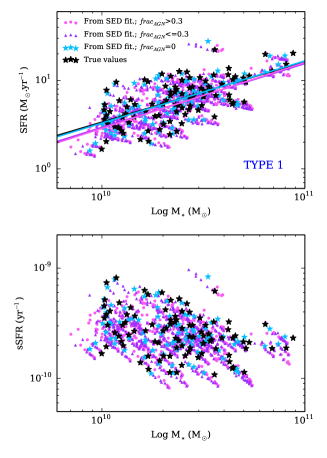
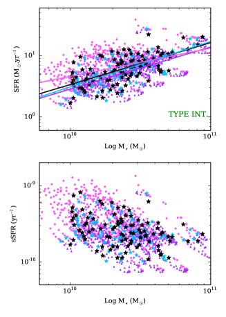
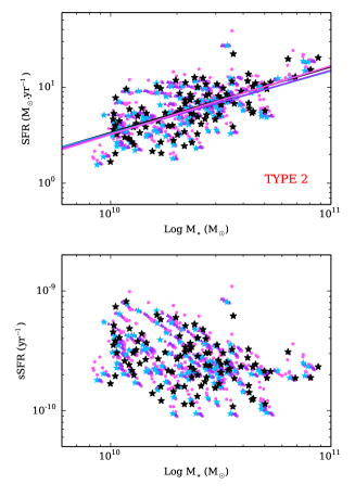
Figure 13: Top panels: SFR-$M_{*}$ diagram for the Type 1 sample (left), the intermediate type (middle), and the Type 2 sample (right) obtained when using the 2$\tau$-dec SFH model for the fitting. Black stars are the true values of the SFR and $M_{*}$ of the mock galaxies. Cyan stars are the galaxies without any AGN component ($frac_{AGN}$=0), purple triangle are galaxies with an AGN contribution lower than 30%, and pink circle galaxies with an AGN contribution higher than 30%. Colored-lines are the linear fit corresponding to each subsample. Bottom panels: sSFR-$M_{*}$ diagram for the Type 1 sample (left), the intermediate type (middle), and the Type 2 sample (right).

5 Comparison against IR-only SED decomposition

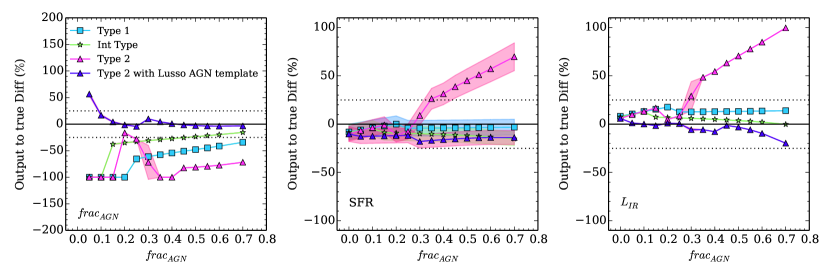
Figure 14: Relative difference between the $frac_{AGN}$ (left panel) and the SFR (right panel) obtained by DecompIR and the true values. Cyan squares, green triangles, and magenta triangles are Type 1, intermediate type, and Type 2 outputs from DecompIR, respectively. The purple triangles present the results provided by DecompIR for the Type 2 mock catalogue obtained using the Lusso et al. (2013) templates. The dotted lines indicate the 25% difference.

In this Section, we use our mock catalogues to test another method used to disentangle the AGN emission from the host galaxy in the IR, DecompIR (Mullaney et al. 2011). The choice of DecompIR is driven by the fact that the code is popular to derive the IR properties of AGN host galaxies and is publicly available. The aim here is not to compare the results obtained from CIGALE and DecompIR as they are two very different methods. Indeed, results from CIGALE are based on energy balance SED fitting using multi wavelength data from UV to submm, whereas DecompIR is based only on the IR. DecompIR uses a set of observed templates for the host and the AGN. The host galaxy templates are derived by using the Brandl et al. (2006) SB sample, as well as four galaxies taken in the Revised Bright Galaxy Sample. These host templates are grouped into five different averages, spanning a wide range of possible observed SB IR SEDs. The AGN template is defined by effectively subtracting these host templates from the IR SEDs of local AGNs (Mullaney et al. 2011).

To determine how successfully DecompIR separates the AGN component from the host emission, and thus estimates the SFR, we perform SED fitting with the five different SB templates and an AGN component using MIPS 24 $\mu$m to SPIRE 500 $\mu$m data, corresponding to 12 to 250 $\mu$m rest frame. For each mock galaxy, we also fit the IR SEDs, using only the five different SB components, i.e. without allowing any AGN contribution. This last test is performed to examine the value of adding an AGN component to the fit. As a result, each mock galaxy is tested with ten different configurations (i.e. 5 double components and 5 single component) for which $\chi^{2}$ are derived.

We then use an Akaike Information Criterion (AIC) to select the best model, regardless the number of components used to fit the data. The AIC is comparable to the more popular Bayesian Information Criterion (BIC). Although both criteria are derived in the same way, the main difference comes from the prior used which is inversely proportional to the number of models for the BIC, and a decreasing function of the number of models for the AIC. However, some advanced studies comparing both criteria, showed that the AIC is more accurate in model selection than the BIC (see Burnham & Anderson (2004) and Yang (2005) for detailed comparisons). For each mock galaxy, we submit the ten different $\chi^{2}$ to the AIC. We find that for the Type 1, intermediate type, and Type 2 AGNs, the AGN components improves the fit for 36, 21 and 47% of the galaxies, respectively. For all of the other galaxies, whatever the type, a SB template is enough. We then estimate the AGN fraction, the $L_{IR}$, and the uncontaminated SFR, using Kennicutt (1998).

Figure 14 shows the results, i.e. the variation of the estimation of the AGN contribution, the SFR and the $L_{IR}$ with the AGN contribution using DecompIR. We present the estimate of the $L_{IR}$ as the SFR is determined from the simple conversion of $L_{IR}$ using Kennicutt (1998). The AGN contribution is always underestimated (except for one point corresponding to $frac_{AGN}$ $\sim$20% in the Type 2 sample). Confirming what observed with the CIGALE results, low fractions of AGN are difficult to constrain. The Type 1 AGN contribution is underestimated by at least 25%, whereas intermediate type $frac_{AGN}$ is closer to the true value with an offset comprised between 15 and 50%. The variation of the estimation of the AGN contribution of the Type 2 sample is however peculiar as it is not monotonic. Like the results obtained with CIGALE, the SFR is slightly underestimated but well recovered whatever the fraction of AGN for the Type 1 and intermediate type sample, and up to 70% for the Type 2 sample. This is linked to the good recovery of the $L_{IR}$ with a small overestimation of a few percent in the absence of AGN, that does not evolve with $frac_{AGN}$ for the intermediate type sample, slightly increases up to $\sim$15% for the Type 1 sample, and follow the peculiar behavior observed for the estimation of $frac_{AGN}$ for the Type 2 sample. However, despite problems in recovering the right contribution of the AGN, SFR of Type 1 and intermediate type AGNs are well recovered.

The estimate of the SFR and $L_{IR}$ of our Type 2 AGN sample by DecompIR is problematic for fractions larger than 40%. One explanation is that Type 2 templates from Fritz et al. (2006) predict IR SED cooler than what was empirically obtained by Mullaney et al. (2011). Thus, when DecompIR tries to fit the Type 2 catalogue created from Fritz et al. (2006) models, the models attribute the excess of FIR emission produced by the Type 2 AGN from Fritz et al. (2006) to star formation, leading to the offset on the $L_{IR}$ that we see in Figure 14. In order to test this point, we run DecompIR on the mock catalogue obtained with the Type 2 AGN template of Lusso et al. (2013) used in Section 3.4. The results are presented in purple in Figure 14. The SFR and $L_{IR}$ are no longer overestimated. DecompIR provides a good estimate of the SFR with a small underestimation between 10 and 20%, as well as for the $L_{IR}$ with an underestimation up to 20% for the highest fraction. Interestingly, the estimate on the contribution of the AGN to the $L_{IR}$ is well constrained and is similar to what obtained with CIGALE, i.e an overestimation of low fractions of about 50%.

6 Conclusions

We simulate realistic SEDs of Type 1, intermediate type, and Type 2 AGNs hosts in order to evaluate the impact of the AGN emission on the host SED, and estimate the ability of SED fitting code to retrieve the physical properties of the galaxy. CIGALE is used to model the SEDs from SFHs provided by the SAM galform code. Three samples are built, one with the emission of a Type 1AGN, one with the emission of an intermediate type AGN, and one with the emission of a Type 2 AGN, varying their contribution through the $frac_{AGN}$ parameter. We use the SED fitting function of the recently updated CIGALE model to derive the stellar mass, star formation rate, and contribution of the AGN of each mock galaxy, assuming three popular shapes of SFH: 1$\tau$-dec, 2$\tau$-dec, and a delayed SFH.

In the absence of an AGN contribution, i.e. in normal galaxies, the SED fitting of our mock samples shows that all the three SFHs considered in this work provide good estimations of the stellar mass within $\sim$10%. The best estimates are obtained using the 2$\tau$-dec model but at the expense of realistic ages of the stellar population, whereas the delayed model provide both. Star formation rates are well recovered within 12%.

For AGNs, the SED fitting of our mock samples shows that:

• Stellar masses are overall well recovered with systematics up to 40% (0.17 dex) or better, depending on the $frac_{AGN}$ and spectral shape of the AGN component. This results is rather insensitive to photometric bands available as long as UV–MIR data are available. $M_{*}$ is therefore the most robust parameter that one can constraint for AGN hosts galaxies via broad-band photometric decomposition.

• The SFR suffers from systematic uncertainties up to 40-50% or better as long as FIR/submm data are available. Data-sets that are limited to the MIR cannot be used to constrain the SFR of AGN hosts.

• AGN/galaxy decomposition based on broad-band photometry can lead to significant overestimation of the AGN fraction and hence the inferred AGN luminosity in the case of weak AGN.

We note the need for UV rest frame data to constrain the stellar mass and star formation rate of Type 1 and intermediate type AGNs.

The AGN emission has an influence on the slope of the MS depending on the SFH assumptions used for the SED fitting and the type of AGN . As the AGN contribution can slightly bias the estimates of $M_{*}$ and SFR, the variety of AGN types and AGN intensities increases the dispersion of the MS. Furthermore, the SFR-$M_{*}$ relation is more sensitive to the estimation of the stellar mass than of the SFR.

Finally, we use our mock samples to test a popular method used to disentangle the AGN emission from the host emission in the IR, DecompIR (Mullaney et al. 2011), and find that, using the mock catalogues built from Fritz et al. (2006) AGN templates, $frac_{AGN}$ is always underestimated but the SFR is well recovered for Type 1 and intermediate types of AGN, and overestimated in Type 2 AGNs when $frac_{AGN}>$35%. The overestimation of the SFR of Type 2 AGNs is due to the FIR prediction of Type 2 AGN from Fritz et al. (2006) which is colder than what observed by Mullaney et al. (2011). When using the Type 2 mock catalogue built from Lusso et al. (2013), DecompIR recovers well the SFR and $L_{IR}$ with an underestimation up to 20%.

In this work, we have validated the use of broad-band SED fitting methods to derive the stellar mass and SFR of AGN host galaxies, as well as the contribution of this AGN to the host galaxy SED. This analysis provides the foundation for future AGN multi-wavelength studies using CIGALE. Indeed, in the near future, the eROSITA X-ray telescope will provide observations of about three millions of X-ray detected AGNs as well as samples of tens of thousands obscured AGNs. These data will provide accurate studies of the relationship between accretion on the SMBH and the host galaxy properties. Multi-wavelength analysis using SED fitting will thus be needed to derive these properties.

Appendix A The need for an AGN component to perform the SED fitting

In this work, we use a SED fitting procedure allowing the possibility of using an AGN component. To understand how omitting to use this component would affect the estimate of the stellar mass and SFR of the host galaxies, we perform a SED fitting, using the 2$\tau$-dec SFH model, and not allowing for the use of AGN templates.

Figure 15 presents the fractional difference between the output parameters and the true ones as a function of the input $frac_{AGN}$. The estimate of the stellar mass of the Type 2 sample is not perturbed by the AGN, as we discuss in this work. The NIR bands are not affected by the AGN emission, thus the stellar mass is well recovered, with or without the use of an AGN component. However, Type 1 and intermediate type SEDs are rapidly affected by the AGN emission, and $M_{*}$ is overestimated by 50% at $frac_{AGN}$=10%. This overestimation reaches up to 150% for $frac_{AGN}$=70% in the case of Type 1 AGNs.

The SFR in intermediate type and Type 2 AGNs is overestimated by 20% up to $frac_{AGN}$=30-40%. This overestimation increases for higher fractions, especially in Type 2 AGNs where it can reach up to 100% The case of Type 1 AGNs is more critical, the SFR is rapidly strongly overestimated up to 300% at $frac_{AGN}$=70%.

The $\chi^{2}_{red}$ distributions shows higher value of the $\chi^{2}_{red}$ by a factor of $\sim$10 compared to the distribution from the fitting using the AGN component (Figure 6).

These results show that not taking into account an AGN component when performing broad band SED fitting of AGN host galaxies results in strong biases in the determination of physical properties such the stellar mass and the star formation rate.

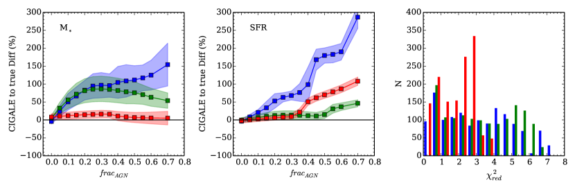
Figure 15: Evolution of the CIGALE to true relative difference of $M_{*}$ and SFR with the fraction of AGN in the case where the AGN component is not taken into account in the fitting procedure. Left panel shows the results for the stellar mass, middle panel for the SFR, and the right panel present the $\chi^{2}_{red}$ distribution. Blue, green, and red data are for Type 1, intermediate type, and Type 2 AGNs, respectively.