Abstract

We present a new well-balanced finite volume method within the framework of the finite volume evolution Galerkin (FVEG) schemes. The methodology will be illustrated for the shallow water equations with source terms modelling the bottom topography and Coriolis forces. Results can be generalized to more complex systems of balance laws. The FVEG methods couple a finite volume formulation with approximate evolution operators. The latter are constructed using the bicharacteristics of multidimensional hyperbolic systems, such that all of the infinitely many directions of wave propagation are taken into account explicitly. We derive a well-balanced approximation of the integral equations and prove that the FVEG scheme is well-balanced for the stationary steady states as well as for the steady jets in the rotational frame. Several numerical experiments for stationary and quasi-stationary states as well as for steady jets confirm the reliability of the well-balanced FVEG scheme.

Key words: well-balanced schemes, steady states, systems of hyperbolic balance laws, shallow water equations, geostrophic balance, evolution Galerkin schemes

AMS Subject Classification: 65L05, 65M06, 35L45, 35L65, 65M25, 65M15

1 Introduction

Consider the balance law in two space dimensions

$$\mbox{\boldmath$u$}_{t}+\mbox{\boldmath$f$}_{1}(\mbox{\boldmath$u$})_{x}+\mbox{\boldmath$f$}_{2}(\mbox{\boldmath$u$})_{y}=\mbox{\boldmath$b$}(\mbox{\boldmath$u$},x,y),$$ (1.1)

where $u$ is the vector of conservative variables, $\mbox{\boldmath$f$}_{1},\,\mbox{\boldmath$f$}_{2}$ are flux functions and $\mbox{\boldmath$b$}(\mbox{\boldmath$u$},x,y)$ is a source term. In this paper we are concerned with the finite volume evolution Galerkin (FVEG) method of Lukáčová, Morton and Warnecke, cf. [22]-[29] and [15]. The FVEG methods couple a finite volume formulation with approximate evolution operators which are based on the theory of bicharacteristics for the first order systems [23]. As a result exact integral representations for solutions of linear or linearized hyperbolic conservation laws can be derived, which take into account all of the infinitely many directions of wave propagation.

In the finite volume framework the approximate evolution operators are used to evolve the solution along the cell interfaces up to an intermediate time level $t_{n+1/2}$ in order to compute fluxes. This step can be considered as a predictor step. In the corrector step the finite volume update is done. The FVEG schemes have been studied theoretically as well as experimentally with respect to their stability and accuracy. Extensive numerical experiments confirm robustness, good multidimensional behaviour, high accuracy, stability, and efficiency of the FVEG schemes, see Section 5 and also references [26, 27]. We refer the reader to [1, 3, 7, 8, 9, 16, 19, 30] for other recent multidimensional schemes.

For balance laws with source terms, the simplest approach is to use the operator splitting method which alternates between the homogeneous conservation laws

$$\mbox{\boldmath$u$}_{t}+\mbox{\boldmath$f$}_{1}(\mbox{\boldmath$u$})_{x}+\mbox{\boldmath$f$}_{2}(\mbox{\boldmath$u$})_{y}=0$$

and the ordinary differential equation

$$\mbox{\boldmath$u$}_{t}=\mbox{\boldmath$b$}(\mbox{\boldmath$u$},x,y)$$

at each time step. For many situations this would be effective and successful. However, the original problem (1.1) has an interesting structure, which is due to the interplay between the differential terms and the right-hand-side source term during the time evolution. For many flows which are of interest in geophysics, the terms are nearly perfect balanced. If these terms are treated separately in a numerical algorithm, the fundamental balance may be destroyed, resulting in spurious oscillations. In particular, we will be interested in approximating correctly equilibrium states or steady states, for which

$$\mbox{\boldmath$f$}_{1}(\mbox{\boldmath$u$})_{x}+\mbox{\boldmath$f$}_{2}(\mbox{\boldmath$u$})_{y}=\mbox{\boldmath$b$}(\mbox{\boldmath$u$},x,y),$$

and we want to approximate perturbations of such equilibrium states. Equilibrium solutions play an important role because they are obtained usually as a limit when time tends to infinity.

In this paper we present an approach which allows to incorporate treatment of the source in the framework of the FVEG schemes without using the operator splitting approach. The key ingredient is a new approximate representation of the multi-dimensional solution which contains the full balance of the hydrostatic pressure and the source terms, see Lemma 3.2. This new representation allows to apply a recent non-standard quadrature rule (see (3.39) and also [27]) to the mantle integrals of the bicharacteristic cone. This leads to a surprisingly simple, accurate and efficient approximate evolution operator and hence to an efficient, accurate and well-balanced finite volume scheme. We call our scheme the well-balanced finite volume evolution Galerkin scheme (FVEG). We refer the reader to [2, 4, 5, 10, 12, 17, 20, 31, 13, 34] and the references therein for other related approaches for well-balanced finite volume and finite difference schemes.

Our paper is organized as follows. In Section 2 we introduce the shallow water equations in a rotating frame, derive a class of equilibria which contains the lake at rest, jets in the rotating frame and combinations of these two solutions. Then we introduce the class of two-step finite volume schemes used throughout the paper. In Theorem 2.1 we give sufficient conditions which guarantee well-balancing. Section 3 is devoted to the EG (evolution Galerkin) predictor step. Applying the theory of bicharacteristics for multidimensional first order systems of hyperbolic type the exact evolution operator is derived. A well-balanced approximation of the exact evolution operator, which preserves some interesting steady states exactly and also works well for their perturbations, is given in Lemma 3.2 and equations (3.43) – (3.44). In Theorem 3.1 we prove that the FVEG scheme is well-balanced for the stationary steady states (e.g. lake at rest), for the steady jets on the rotating plane as well as for combinations of these two flows. In Section 4 we summarize the main steps of the FVEG method and present its algorithm. Numerical experiments for one and two-dimensional stationary and quasi-stationary problems as well as for steady jets presented in Section 5 confirm reliability of the well-balanced FVEG scheme. We also compare the accuracy and runtime of the new FVEG scheme with that of the recent high order well-balanced WENO FV schemes of Audusse et a. [2] and Noelle et al. [31]. The question of positivity preserving property of the scheme, i.e. $h>0$, is not yet considered here and will be addressed in our future paper.

2 Geophysical equilibria and well-balanced two-step finite volume schemes

2.1 The shallow water equations

There are many practical applications where the balance laws and the correct approximation of their quasi-steady states are necessary. Some example include shallow water equations with the source term modelling the bottom topography, which arise in oceanography and atmospheric science, gas dynamic equations with geometrical source terms, e.g. a duct with variable cross-section, or fluid dynamics with gravitational terms. In what follows we illustrate the methodology on the example of the shallow water equations with the source terms modelling the bottom topography and the Coriolis forces. This system reads

$$\mbox{\boldmath$u$}_{t}+\mbox{\boldmath$f$}_{1}(\mbox{\boldmath$u$})_{x}+\mbox{\boldmath$f$}_{2}(\mbox{\boldmath$u$})_{y}=\mbox{\boldmath$b$}(\mbox{\boldmath$u$}),$$ (2.1)

where

$$u = \left(\begin{array}[]{c}h\\ hu\\ hv\end{array}\right),\ \mbox{\boldmath$f$}_{1}(\mbox{\boldmath$u$})=\left(\begin{array}[]{c}hu\\ hu^{2}+\frac{1}{2}gh^{2}\\ huv\end{array}\right),$$ (2.8)

$$\mbox{\boldmath$f$}_{2}(\mbox{\boldmath$u$}) = \left(\begin{array}[]{c}hv\\ huv\\ hv^{2}+\frac{1}{2}gh^{2}\end{array}\right),\ \mbox{\boldmath$b$}(\mbox{\boldmath$u$})=\left(\begin{array}[]{c}0\\ -ghb_{x}+fhv\\ -ghb_{y}-fhu\end{array}\right).$$ (2.15)

Here $h$ denotes the water depth, $u,v$ are vertically averaged velocity components in $x-$ and $y-$ direction, $g$ stands for the gravitational constant, $f$ is the Coriolis parameter, and $b(x,y)$ denotes the bottom topography.

Note that these equations are also used in climate modelling and meteorology for geostrophic flow, see, e.g., [4, 14]. For simulation of river or oceanographic flows some additional terms modelling the bottom friction need to be considered as well.

2.2 Equilibria

Many geophysical flows are close to equilibrium, or stationary state. It is easiest to identify these states when the system is written in primitive variables,

$$\mbox{\boldmath$w$}_{t}+\mbox{\boldmath$A$}_{1}(\mbox{\boldmath$w$})\mbox{\boldmath$w$}_{x}+\mbox{\boldmath$A$}_{2}(\mbox{\boldmath$w$})\mbox{\boldmath$w$}_{y}=\mbox{\boldmath$t$}(\mbox{\boldmath$w$}),$$ (2.16)

$$\mbox{\boldmath$w$}=\left(\begin{array}[]{c}h\\ u\\ v\\ \end{array}\right),\mbox{\boldmath$A$}_{1}=\left(\begin{array}[]{ccc}u&h&0\\ g&u&0\\ 0&0&u\\ \end{array}\right),\mbox{\boldmath$A$}_{2}=\left(\begin{array}[]{cccc}v&0&h\\ 0&v&0\\ g&0&v\\ \end{array}\right),\mbox{\boldmath$t$}=\left(\begin{array}[]{c}0\\ -gb_{x}+fv\\ -gb_{y}-fu\end{array}\right).$$ (2.29)

Here we consider states which are both stationary,

$$(h,u,v)_{t}=0,$$ (2.30)

and constant along streamlines,

$$(\dot{h},\dot{u},\dot{v})=0,$$ (2.31)

where $\;\dot{}=\partial_{t}+u\partial_{x}+v\partial_{y}$ is the material derivative. For such states, we obtain

$$uh_{x}+vh_{y}=uu_{x}+vu_{y}=uv_{x}+vv_{y}=0.$$ (2.32)

Since the velocity vector is now constant along the streamlines, these become straight lines. It is then natural to align the coordinates with the streamlines. The desired solution has to satisfy the conditions

$$u =0$$ (2.33)

$$v_{y} =0$$ (2.34)

$$vh_{y} =0$$ (2.35)

$$g(h+b)_{x} =fv$$ (2.36)

$$g(h+b)_{y} =0.$$ (2.37)

In the region $\{(x,y)|\,v(x)=0\}$ we obtain the lake at rest solution, where the water level $h+b$ is flat. When $v(x)\neq 0$, we must have $h_{y}$ = 0 and hence $b_{y}=0$. Hence the topography is locally one-dimensional, and along the rise of the bottom we have a one-dimensional flow. This solution, which is well-known to oceanographers, is called the jet in the rotational frame. Due to the earths rotation the jet exerts a sidewards pressure $fv$ onto the water, which is balanced by a raise in the water level $g(h+b)_{x}$. In meteorological literature this state is also called the geostrophic equilibrium.

For future reference we also define the primitive $(U,V)$ of the Coriolis force, as introduced by Bouchut et al. in [2], via

$$V_{x}=\frac{f}{g}v\quad\mbox{and}\quad U_{y}=\frac{f}{g}u$$ (2.38)

and the potential energies

$$K:=g(h+b-V)\quad\mbox{and}\quad L:=g(h+b+U).$$ (2.39)

2.3 Two-step finite volume schemes

The FVEG (Finite Volume Evolution Galerkin) scheme which we propose for the balance laws are time-explicit two-step schemes, similarly as Richtmyer’s two-step version of the Lax-Wendroff scheme [32] and Colella’s CTU (corner transport upwind) scheme [6].

The first step, called predictor step, evolves the point value at a quadrature node to the half-timestep. This can be done by a simple finite difference operator as in [32], by one-dimensional characteristic theory as in [6] or by fully multidimensional, bicharacteristic theory as in [25] and related works of Lukáčová, Morton, Warnecke et al.. Our predictor step is based on this bicharacteristic theory.

The second step is the standard finite volume update. It approximates the flux integral across the interfaces by a quadrature of the fluxes evaluated at the predicted states at the half-timestep.

We proceed as follows: in the present section we study the finite volume step (i.e. the second of the two steps). This will give us sufficient conditions for well-balancing which should be satisfied by the values computed in the predictor step (the first step). In Section 3.1 we will introduce the evolution Galerkin predictor step and prove that it satisfies the sufficient conditions derived in the present section.

In order to define the class of two step finite volume schemes, let us divide a computational domain $\Omega$ into a finite number of regular finite volumes $\Omega_{ij}=[x_{i-\frac{1}{2}},x_{i+\frac{1}{2}}]\times[y_{j-\frac{1}{2}},y_{j+\frac{1}{2}}]=[x_{i}-\hbar/2,x_{i}+\hbar/2]\times[y_{j}-\hbar/2,y_{j}+\hbar/2]$, $i,j\in\mathbb{Z}$, where $\hbar$ is the mesh size. Denote by $\mbox{\boldmath$U$}_{ij}^{n}$ the piecewise constant approximate solution on a mesh cell $\Omega_{ij}$ at time $t_{n}$ and start with initial approximations obtained by the integral averages $\mbox{\boldmath$U$}_{ij}^{0}=\int_{\Omega_{ij}}\mbox{\boldmath$U$}(\cdot,0)$. Integrating the balance law (2.1) and applying the Gauss theorem on any mesh cell $\Omega_{ij}$ yields the following finite volume update formula

$$\mbox{\boldmath$U$}_{ij}^{n+1}=\mbox{\boldmath$U$}_{ij}^{n}-\lambda\sum_{k=1}^{2}\delta^{ij}_{x_{k}}\bar{\mbox{\boldmath$f$}}_{k}^{n+1/2}+\lambda\mbox{\boldmath$B$}_{ij}^{n+1/2},$$ (2.40)

where $\lambda=\Delta t/\hbar$, $\Delta t$ is a time step, $\delta^{ij}_{x_{k}}$ stands for the central difference operator in the $x_{k}$-direction, $k=1,2$ and $\bar{\mbox{\boldmath$f$}}_{k}^{n+1/2}$ represents an approximation to the edge flux at the intermediate time level $t_{n}+\Delta t/2$. Further $\mbox{\boldmath$B$}_{ij}^{n+1/2}$ stands for the approximation of the source term multiplied with the mesh size, $\hbar\mbox{\boldmath$b$}$. The cell interface fluxes $\bar{\mbox{\boldmath$f$}}_{k}^{n+1/2}$ are evolved using an approximate evolution operator denoted by $E_{\Delta t/2}$ to $t_{n}+\Delta t/2$ and averaged along the cell interface edge denoted by ${\cal E}$,

$$\bar{\mbox{\boldmath$f$}}_{k}^{n+1/2}:=\sum_{j}\omega_{j}\mbox{\boldmath$f$}_{k}(E_{\Delta t/2}\mbox{\boldmath$U$}^{n}(\mbox{\boldmath$x$}^{j}({\cal E}))).$$ (2.41)

Here $\mbox{\boldmath$x$}^{j}({\cal E})$ are the nodes and $\omega_{j}$ the weights of the quadrature for the flux integration along the edges.

For simplicity, we introduce the following notation. Along the edges, we have quadrature nodes $(x_{i\pm\frac{1}{2}},y_{j+j^{\prime}})$ resp. $(x_{i+i^{\prime}},y_{j\pm\frac{1}{2}})$, where $i^{\prime},j^{\prime}\in\{0,\pm\frac{1}{2}\}$. These nodes are already sufficient for the midpoint, the trapezoidal and Simpson’s rule. We denote the values given at the predictor step by

$$\left(\!\!\begin{array}[]{c}\hat{h}\\ \hat{u}\\ \hat{v}\end{array}\!\right)_{i\pm\frac{1}{2},j+j^{\prime}}\!\!\!\! :=\left(\!\!\begin{array}[]{c}h\\ u\\ v\end{array}\!\right)_{i\pm\frac{1}{2},j+j^{\prime}}^{n+\frac{1}{2}}\quad\mathrm{and}\quad\left(\!\!\begin{array}[]{c}\hat{h}\\ \hat{u}\\ \hat{v}\end{array}\!\right)_{i+i^{\prime},j\pm\frac{1}{2}}\!\!\!\!:=\left(\!\!\begin{array}[]{c}h\\ u\\ v\end{array}\!\right)_{i+i^{\prime},j\pm\frac{1}{2}}^{n+\frac{1}{2}}$$ (2.54)

and the corresponding fluxes in $x$ resp. $y$-direction by

$$\mbox{\boldmath$\hat{f}$}^{1}_{i\pm\frac{1}{2},j+j^{\prime}} :=\mbox{\boldmath$f$}_{1}((\hat{h},\hat{u},\hat{v})_{i\pm\frac{1}{2},j+j^{\prime}})$$ (2.55)

$$\mbox{\boldmath$\hat{f}$}^{2}_{i+i^{\prime},j\pm\frac{1}{2}} :=\mbox{\boldmath$f$}_{2}((\hat{h},\hat{u},\hat{v})_{i+i^{\prime},j\pm\frac{1}{2}}).$$ (2.56)

With this notation, we obtain

$$\delta^{ij}_{x_{1}}\bar{\mbox{\boldmath$f$}}_{1}^{n+1/2} =\sum_{j^{\prime}}\omega_{j^{\prime}}\delta^{i,j+j^{\prime}}_{x_{1}}\mbox{\boldmath$\hat{f}$}^{1}_{i,j+j^{\prime}}$$ (2.57)

$$\delta^{ij}_{x_{2}}\bar{\mbox{\boldmath$f$}}_{2}^{n+1/2} =\sum_{i^{\prime}}\omega_{i^{\prime}}\delta^{i+i^{\prime},j}_{x_{2}}\mbox{\boldmath$\hat{f}$}^{2}_{i+i^{\prime},j}.$$ (2.58)

Finally we discretize the source term by

$$\mbox{\boldmath$B$}_{ij}^{n+\frac{1}{2}}=-\;g\left(\!\!\begin{array}[]{c}0\\ \sum_{j^{\prime}}\omega_{j^{\prime}}\;(\mu^{i,j+j^{\prime}}_{x_{1}}\;\hat{h}_{i,j+j^{\prime}})\;(\delta^{i,j+j^{\prime}}_{x_{1}}\;(\hat{b}-\hat{V})_{i,j+j^{\prime}})\\[4.30554pt] \sum_{i^{\prime}}\omega_{i^{\prime}}\;(\mu^{i+i^{\prime},j}_{x_{2}}\;\hat{h}_{i+i^{\prime},j})\;(\delta^{i+i^{\prime},j}_{x_{2}}\;(\hat{b}+\hat{U})_{i+i^{\prime},j})\end{array}\!\right).$$ (2.59)

Here $U$ and $V$ are the discrete primitives of the Coriolis forces (see (2.38)), defined by

$$\delta^{i,j+j^{\prime}}_{x_{1}}\hat{V}_{i,j+j^{\prime}} =\hbar\frac{f}{g}\;\mu^{ij}_{x_{1}}\hat{v}_{i,j+j^{\prime}}$$ (2.60)

$$\delta^{i+i^{\prime},j}_{x_{2}}\hat{U}_{i+i^{\prime},j} =\hbar\frac{f}{g}\;\mu^{i+i^{\prime},j}_{x_{2}}\hat{u}_{i+i^{\prime},j},$$ (2.61)

and we have used the average operators

$$\mu^{ij}_{x_{1}}a =(a_{i+1/2,j}+a_{i-1/2,j})/2$$

$$\mu^{ij}_{x_{2}}a =(a_{i,j+1/2}+a_{i,j-1/2})/2.$$

The following theorem states conditions which guarantee that the two-step finite volume scheme (2.40) – (2.41) is well-balanced for the lake at rest as well as for the jet in the rotating frame.

Theorem 2.1.

Suppose that the values $(\hat{h},\hat{u},\hat{v})$ given by predictor step satisfy for all $i,j,i^{\prime},j^{\prime}$

$$\hat{u}_{i,j+j^{\prime}} = 0$$ (2.62)

$$\delta_{y}^{i+i^{\prime},j}\hat{v}_{i+i^{\prime},j} = 0$$ (2.63)

$$\hat{v}_{i+i^{\prime},j}\;\delta_{y}^{i+i^{\prime},j}\hat{h}_{i+i^{\prime},j} = 0$$ (2.64)

$$\delta_{x}^{i,j+j^{\prime}}\hat{K}_{i,j+j^{\prime}} = 0$$ (2.65)

$$\delta_{y}^{i+i^{\prime},j}(\hat{h}_{i+i^{\prime},j}+b_{i+i^{\prime},j}) = 0$$ (2.66)

where $K$ is defined in (2.39). Then the finite volume scheme preserves the lake at rest and the jet in the rotating frame.

Proof.

Since this argument is already standard for the lake at rest, we only sketch it briefly for the jet in the rotating frame. Let us study conservation of momentum in the $y$-direction over cell $\Omega_{ij}$. Using (2.62) – (2.64), (2.66), and the discrete product rule

$$\delta(\hat{a}\hat{b}) =\delta(\hat{a})\mu(\hat{b})+\mu(\hat{a})\delta(\hat{b})$$ (2.67)

it is straightforward to show that the sum of the flux differences and the source term vanishes:

$$\;(hv)_{ij}^{n+1}-(hv)_{ij}^{n}$$

$$= \;\sum_{j^{\prime}}\omega_{j^{\prime}}\;\delta_{x}^{i,j+j^{\prime}}(\hat{h}\hat{u}\hat{v})+\sum_{i^{\prime}}\omega_{i^{\prime}}\left(\delta_{y}^{i+i^{\prime},j}(\hat{h}\hat{v}^{2}+\frac{g}{2}\hat{h}^{2})+\;g\;(\mu_{y}^{i+i^{\prime},j}\hat{h})\;\delta_{y}^{i+i^{\prime},j}(b+\hat{U})\right).$$ (2.68)

Now $\hat{u}_{i\pm\frac{1}{2},j+j^{\prime}}=0$, and

$$\quad\delta_{y}^{i+i^{\prime},j}(\hat{h}\hat{v}^{2}) =\delta_{y}^{i+i^{\prime},j}(\hat{h}\hat{v})\;\mu_{y}^{i+i^{\prime},j}\hat{v}+\mu_{y}^{i+i^{\prime},j}(\hat{h}\hat{v})\;\delta_{y}^{i+i^{\prime},j}\hat{v}$$

$$=\delta_{y}^{i+i^{\prime},j}\hat{h}\;\mu_{y}^{i+i^{\prime},j}\hat{v}+\mu_{y}^{i+i^{\prime},j}\hat{\;}\delta_{y}^{i+i^{\prime},j}\hat{v}$$

$$=0.$$

Dropping the corresponding terms in (2.68), we obtain

$$(hv)_{ij}^{n+1}-(hv)_{ij}^{n} =\;\sum_{i^{\prime}}\omega_{i^{\prime}}\;(\mu_{y}^{i+i^{\prime},j}\hat{h})\;\delta_{y}^{i+i^{\prime},j}g(\hat{h}+b+\hat{U})$$

$$=\;\sum_{i^{\prime}}\omega_{i^{\prime}}\;(\mu_{y}^{i+i^{\prime},j}\hat{h})\;\delta_{y}^{i+i^{\prime},j}\hat{L}$$

$$=\;\;0.$$

This is the desired well-balanced property for the $y$-momentum. The $x$-momentum and the balance of mass can be treated analogously.  

3 The well-balanced approximate evolution operators

The predictor step in the FVEG scheme will be based on exact and approximate integral representations of solutions to the linearized shallow water equations. We begin this section by formulating the exact integral representation. A few clarifying remarks should help the reader to understand the structure of this representation. Details of the derivation are given in Appendix A. We proceed to derive two approximate integral representations. For the first order scheme the approximate evolution operator $E_{\Delta t/2}^{const}$ for the piecewise constant data is used. For the second order method the continuous bilinear recovery $R$ is applied. In the case of discontinuous solutions slopes in $R$ are limited yielding a discontinuous piecewise bilinear recovery $R$, cf. Section 4 as well as [26]. The predicted solution at the quadrature nodes on the cell interfaces at the half timestep is obtained by a suitable combination of $E_{\Delta}^{const}$ and $E_{\Delta}^{bilin}$,

$$E_{\Delta t/2}\mbox{\boldmath$U$}^{n}:=E^{bilin}_{\Delta t/2}R\mbox{\boldmath$U$}^{n}+E^{const}_{\Delta t/2}(1-\mu_{x}^{2}\mu_{y}^{2})\mbox{\boldmath$U$}^{n},$$ (3.1)

where $\mu_{x}^{2}U_{ij}=1/4(U_{i+1,j}+2U_{ij}+U_{i-1,j})$; an analogous notation is used for the $y-$direction. It has been shown in [27] that the combination (3.1) yields the best results with respect to accuracy as well as stability among other possible second order FVEG schemes. It is particularly important that the constant evolution term $E^{const}_{\Delta t/2}(1-\mu_{x}^{2}\mu_{y}^{2})\mbox{\boldmath$U$}^{n}$ corrects the conservativity of the bilinear recovery and hence of the intermediate solutions along cell-interfaces. If it is not used the scheme is second order formally, but unconditionally unstable, cf. the FVEG-B scheme [27].

Finally we show that approximate evolution operators lead to well-balanced two-step finite volume schemes for the lake at rest and the jet in the rotational frame.

3.1 Exact integral representation

We believe that the most satisfying methods for evolutionary problems are based on the approximation of evolution operator or at least its dominant part. For the two-step FVEG method, we use two fundamental evolution operators. One of the steps is the classical finite volume update for the cell averages and uses the integral form of the conservation law. Its well-balanced properties have been established in Theorem 2.1. The other step, which precedes the finite volume update, is needed to predict point values in order to evaluate fluxes on cell interfaces. It is here that the classical bicharacteristic theory comes into play. It provides exact integral formulae for point values of solutions to multidimensional hyperbolic systems.

Let $P:=(x,y,t_{n+1/2})$ be one of the quadrature points where the finite volume fluxes will be evaluated, and let $\tilde{w}=(\tilde{h},\tilde{u},\tilde{v})$ be a suitable local average of the solution around $P$. We will derive an exact integral representation of the solution of the linearized shallow water equation at $P$. Similarly as in (2.16), the linearized system in primitive variables reads

$$\mbox{\boldmath$w$}_{t}+\mbox{\boldmath$A$}_{1}(\mbox{\boldmath$\tilde{w}$})\mbox{\boldmath$w$}_{x}+\mbox{\boldmath$A$}_{2}(\mbox{\boldmath$\tilde{w}$})\mbox{\boldmath$w$}_{y}=\mbox{\boldmath$t$}(\mbox{\boldmath$w$}),$$ (3.2)

where the Jacobian matrices $A_{1}$ and $A_{2}$ are defined in (2.29).

The homogeneous part of (3.2) yields a hyperbolic system. Fix a direction angle $\theta$ with corresponding unit normal vector $(\cos\theta,\sin\theta)$. The matrix pencil $\mbox{\boldmath$A$}\equiv\mbox{\boldmath$A$}(\mbox{\boldmath$\tilde{w}$})=\cos\theta\mbox{\boldmath$A$}_{1}+\sin\theta\mbox{\boldmath$A$}_{2}$, has three eigenvalues

$$\lambda_{1} = \cos\theta\,\tilde{u}+\sin\theta\,\tilde{v}-\tilde{c},$$

$$\lambda_{2} = \cos\theta\,\tilde{u}+\sin\theta\,\tilde{v},$$

$$\lambda_{3} = \cos\theta\,\tilde{u}+\sin\theta\,\tilde{v}+\tilde{c},$$

and a full set of right eigenvectors

$$\mbox{\boldmath$r$}_{1}=\left(\begin{array}[]{c}-1\\ g\cos\theta/\tilde{c}\\ g\sin\theta/\tilde{c}\\ \end{array}\right),\>\>\mbox{\boldmath$r$}_{2}=\left(\begin{array}[]{c}0\\ \sin\theta\\ -\cos\theta\\ \end{array}\right),\>\>\mbox{\boldmath$r$}_{3}=\left(\begin{array}[]{c}1\\ g\cos\theta/\tilde{c}\\ g\sin\theta/\tilde{c}\\ \end{array}\right),$$

where $c=\sqrt{gh}$ denotes the wave celerity. The eigenvalues $\lambda_{1,3}$ correspond to fast waves, the so-called inertia-gravity waves, whereas slow modes are related to $\lambda_{2}$. Analogously to the gas dynamics the Froude number $Fr=|\mbox{\boldmath$u$}|/c$ plays an important role in the classification of shallow flows. The shallow flow is called supercritical, critical or subcritical for $Fr>1,Fr=1,$ and $Fr<1$, respectively.

Applying the theory of bicharacteristics to the linearized system (3.2) yields an exact integral representation of the solution. Since the computations are closely related to [27], we summarize the key steps only briefly and refer to Appendix A for further details.

• Fix a point $P=(x,y,t_{n}+\tau)$,  $\tau=\frac{\Delta t}{2}$.

  For each spatial direction $(\cos(\theta),\sin(\theta)),\theta\in[0,2\pi)$ apply the corresponding one-dimensional characteristic decomposition to two-dimensional system (3.2).

• Integrate the resulting equations along each bicharacteristic curve from time $t_{n}$ to time $t_{n}+\tau$.

• Integrate the resulting equations over all direction angles $\theta$. This gives a representation formula for the solution at the point $P$.

Figure 1: Bicharacterestics cone.

The EG integral representation derived in Appendix A then reads, cf. (A)-(A)

$$h\left(P\right) = \frac{1}{2\pi}\int_{0}^{2\pi}h\left(Q\right)-\frac{\tilde{c}}{g}\left(u\left(Q\right)\cos\theta+v\left(Q\right)\sin\theta\right)\mbox{d}\theta\phantom{mmmmmmmmmmmmmmmm}$$

$$-\frac{1}{2\pi}\int_{t_{n}}^{t_{n}+\tau}\frac{1}{t_{n}+\tau-\tilde{t}}\int_{0}^{2\pi}\frac{\tilde{c}}{g}\left(u(\tilde{Q})\cos\theta+v(\tilde{Q})\sin\theta\right)\mbox{d}\theta\mbox{d}\tilde{t}$$

$$+\frac{1}{2\pi}\tilde{c}\int_{t_{n}}^{t_{n}+\tau}\int_{0}^{2\pi}\left(b_{x}(\tilde{Q})\cos\theta+b_{y}(\tilde{Q})\sin\theta\right)\mbox{d}\theta\mbox{d}\tilde{t}$$

$$-\frac{1}{2\pi}\frac{\tilde{c}f}{g}\int_{t_{n}}^{t_{n}+\tau}\int_{0}^{2\pi}\left(v(\tilde{Q})\cos\theta-u(\tilde{Q})\sin\theta\right)\mbox{d}\theta\mbox{d}\tilde{t},$$

$$u\left(P\right) = \frac{1}{2}u\left(Q_{0}\right)+\frac{1}{2\pi}\int_{0}^{2\pi}-\frac{g}{\tilde{c}}h\left(Q\right)\cos\theta+u\left(Q\right)\cos^{2}\theta+v\left(Q\right)\sin\theta\cos\theta\,\mbox{d}\theta$$

$$-\frac{g}{2}\int_{t_{n}}^{t_{n}+\tau}\left(h_{x}(\tilde{Q}_{0})+b_{x}(\tilde{Q}_{0})\right)\mbox{d}\tilde{t}$$

$$-\frac{g}{2\pi}\int_{t_{n}}^{t_{n}+\tau}\int_{0}^{2\pi}\left(b_{x}(\tilde{Q})\cos^{2}\theta+b_{y}(\tilde{Q})\sin\theta\cos\theta\right)\mbox{d}\theta\mbox{d}\tilde{t}$$

$$+\frac{1}{2\pi}\int_{t_{n}}^{t_{n}+\tau}\frac{1}{t_{n}+\tau-\tilde{t}}\int_{0}^{2\pi}\left(u(\tilde{Q})\cos 2\theta+v(\tilde{Q})\sin 2\theta\right)\mbox{d}\theta\mbox{d}\tilde{t}$$

$$+\frac{f}{2}\int_{t_{n}}^{t_{n}+\tau}v(\tilde{Q}_{0})\mbox{d}\tilde{t}+\frac{f}{2\pi}\int_{t_{n}}^{t_{n}+\tau}\int_{0}^{2\pi}\left(v(\tilde{Q})\cos^{2}\theta-u(\tilde{Q})\sin\theta\cos\theta\right)\mbox{d}\theta\mbox{d}\tilde{t},$$

$$v\left(P\right) = \frac{1}{2}v\left(Q_{0}\right)+\frac{1}{2\pi}\int_{0}^{2\pi}-\frac{g}{\tilde{c}}h\left(Q\right)\sin\theta+u\left(Q\right)\sin\theta\cos\theta+v\left(Q\right)\sin^{2}\theta\,\mbox{d}\theta$$

$$-\frac{g}{2}\int_{t_{n}}^{t_{n}+\tau}\left(h_{y}(\tilde{Q}_{0})+b_{y}(\tilde{Q}_{0})\right)\mbox{d}\tilde{t}$$

$$-\frac{g}{2\pi}\int_{t_{n}}^{t_{n}+\tau}\int_{0}^{2\pi}\left(b_{x}(\tilde{Q})\sin\theta\cos\theta+b_{y}(\tilde{Q})\sin^{2}\theta\right)\mbox{d}\theta\mbox{d}\tilde{t}$$

$$+\frac{1}{2\pi}\int_{t_{n}}^{t_{n}+\tau}\frac{1}{t_{n}+\tau-\tilde{t}}\int_{0}^{2\pi}\left(u(\tilde{Q})\sin 2\theta-v(\tilde{Q})\cos 2\theta\right)\mbox{d}\theta\mbox{d}\tilde{t}$$

$$-\frac{f}{2}\int_{t_{n}}^{t_{n}+\tau}u(\tilde{Q}_{0})\mbox{d}\tilde{t}+\frac{f}{2\pi}\int_{t_{n}}^{t_{n}+\tau}\int_{0}^{2\pi}\left(v(\tilde{Q})\sin\theta\cos\theta-u(\tilde{Q})\sin^{2}\theta\right)\mbox{d}\theta\mbox{d}\tilde{t}.$$

Evolution takes place along the bicharacteristic cone, see Fig. 1, where $P=(x,y,t_{n}+\tau)$ is the peak of the bicharacteristic cone, $Q_{0}=(x-\tilde{u}\tau,y-\tilde{v}\tau,t_{n})$ denotes the center of the sonic circle at time $t_{n}$, $\tilde{Q}_{0}=(x-\tilde{u}(t_{n}+\tau-\tilde{t}),y-\tilde{v}(t_{n}+\tau-\tilde{t}),\tilde{t})$, $\tilde{Q}=(x-\tilde{u}(t_{n}+\tau-\tilde{t})+c(t_{n}+\tau-\tilde{t})\cos\theta,y-\tilde{v}(t_{n}+\tau-\tilde{t})+c(t_{n}+\tau-\tilde{t})\sin\theta,\tilde{t})$ stays for arbitrary point on the mantle and $Q=Q(\tilde{t})\Big{|}_{\tilde{t}=t_{n}}$ denotes a point at the perimeter of the sonic circle at time $t_{n}.$

At first view, it may seem difficult to interpret the terms in (3.1)-(3.1). However, even if one is not familiar with bicharacteristic theory, there is a simple explanation of all terms, which we sketch in the following paragraph.

3.2 A simple interpretation of the EG integral representation

Our interpretation of the EG integral representation is based on a comparison with the approximate representation of the solution which results from a Taylor expansion along the streamlines.

The streamlines of the linearized shallow water equations are given by $\{(x(t),y(t),t)|\dot{x}=\tilde{u},\dot{y}=\tilde{v}\}$. As in Section 2.2, let $\dot{\varphi}:=\varphi_{t}+\tilde{u}\varphi_{x}+\tilde{v}\varphi_{y}$ be the material derivative of a function $\varphi:\bar{D}\to\mathbb{R}$.

Then the linearized shallow water equations (3.1) reduce to

$$\dot{h} =-\tilde{h}(u_{x}+v_{y})$$ (3.6)

$$\dot{u} =-K_{x}$$ (3.7)

$$\dot{v} =-L_{y}.$$ (3.8)

This implies that

$$\ddot{h} =-\tilde{h}(\dot{u}_{x}+\dot{v}_{y})=\tilde{h}(K_{xx}+L_{yy})$$ (3.9)

$$\ddot{u} =-\dot{K}_{x}=g\tilde{h}(u_{x}+v_{y})_{x}-g(\tilde{u}b_{x}+\tilde{v}b_{y})_{x}+fL_{y}$$ (3.10)

$$\ddot{v} =-\dot{L}_{y}=g\tilde{h}(u_{x}+v_{y})_{y}-g(\tilde{u}b_{x}+\tilde{v}b_{y})_{y}-fK_{x},$$ (3.11)

so the exact solution derived in (3.1)-(3.1) can be approximated (up to ${\cal O}(\Delta t^{3})$) by

$$\left(\!\!\begin{array}[]{c}h_{1}\\ u_{1}\\ v_{1}\end{array}\!\right) :=\left(\!\!\begin{array}[]{c}h\\ u\\ v\end{array}\!\right)_{\!\!\!\!\!Q_{0}}\!\!\!-\tau\left(\!\!\begin{array}[]{c}\tilde{h}(u_{x}+v_{y})\\ K_{x}\\ L_{y}\end{array}\!\right)_{\!\!\!\!\!Q_{0}}\!\!\!+\frac{\tau^{2}}{2}\left(\!\!\begin{array}[]{c}\tilde{h}(K_{xx}+L_{yy})\\ g\tilde{h}(u_{x}+v_{y})_{x}-g(\tilde{u}b_{x}+\tilde{v}b_{y})_{x}+fL_{y}\\ g\tilde{h}(u_{x}+v_{y})_{y}-g(\tilde{u}b_{x}+\tilde{v}b_{y})_{y}-fK_{x}\end{array}\!\right)_{\!\!\!\!\!Q_{0}}\!\!\!\!.$$ (3.24)

Now we will indicate how to compare the RHS of the integral representation (3.1)-(3.1) with that of (3.24). We will show that they agree up to terms of ${\cal O}(\Delta t^{3})$. For this we need the following Taylor expansions on the sonic circle and the bicharacteristic cone. For simplicity we introduce the notation

$$\alpha:=\cos\theta,\quad\beta:=\sin\theta.$$

Lemma 3.1.

(Taylor expansions on the sonic circle and the bicharacteristic cone) Let $\varphi:C^{m+1}(\bar{D};\mathbb{R})$ and $\varphi_{0}:=\varphi(Q_{0})$, $\tilde{\varphi}_{0}:=\varphi(\tilde{Q}_{0})$. Then

$$\,\frac{1}{2\pi}\int_{0}^{2\pi}\!\!\alpha^{m}\beta^{n}\varphi d\theta =\sum\limits_{k,l=0}^{k+l\leq m}\frac{\,\frac{1}{2\pi}\int_{0}^{2\pi}\alpha^{k+m}\beta^{l+n}d\theta}{k!l!}(\tilde{c}\tau)^{k+l}\,\partial_{x}^{k}\partial_{y}^{l}\varphi_{0}+\mathcal{O}(\Delta t^{m+1})$$ (3.25)

$$\frac{1}{2\pi\tau}\int_{t_{n}}^{t_{n}+\tau}\!\!\!\!\int_{0}^{2\pi}{\!\!\alpha^{m}\beta^{n}\varphi}\mbox{d}\theta\mbox{d}\tilde{t} =\sum\limits_{k,l=0}^{k+l\leq m}\frac{\,\frac{1}{2\pi}\int_{0}^{2\pi}\alpha^{k+m}\beta^{l+n}d\theta}{k!l!}\frac{1}{\tau}\int_{t_{n}}^{t_{n}+\tau}\left(\tilde{c}(t_{n}+\tau-\tilde{t})\right)^{k+l}\,\partial_{x}^{k}\partial_{y}^{l}\tilde{\varphi}_{0}\mbox{d}\tilde{t}$$

$$\quad+\mathcal{O}(\Delta t^{m+1}).$$ (3.26)

Moreover, $\,\frac{1}{2\pi}\int_{0}^{2\pi}\alpha^{k+m}\beta^{l+n}d\theta=0$ if either $k$ or $l$ are odd integers, and

$$\,\frac{1}{2\pi}\int_{0}^{2\pi}\alpha^{2}d\theta=\,\frac{1}{2\pi}\int_{0}^{2\pi}\beta^{2}d\theta =\frac{1}{2},$$ (3.27)

$$\quad\,\frac{1}{2\pi}\int_{0}^{2\pi}\alpha^{4}d\theta=\,\frac{1}{2\pi}\int_{0}^{2\pi}\beta^{4}d\theta =\frac{3}{8},$$ (3.28)

$$\quad\,\frac{1}{2\pi}\int_{0}^{2\pi}\alpha^{2}\beta^{2}d\theta =\frac{1}{8}.$$ (3.29)

Proof.

can be obtained by a direct evaluation.  

Using this Taylor expansion together with appropriate smoothness assumptions it is an elementary exercise to prove that

$$\left(\!\!\begin{array}[]{c}h_{1}\\ u_{1}\\ v_{1}\end{array}\!\right) =\left(\!\!\begin{array}[]{c}h\\ u\\ v\end{array}\!\right)\!\!(P)+{\cal O}(\Delta t^{3}).$$ (3.36)

3.3 Approximate evolution operators

In the previous section, we could give the integral representation (3.1) – (3.1) a straightforward interpretation by deriving it from a Taylor expansion along the streamlines.

However, it would be far too expensive to evaluate (3.1) – (3.1) at each quadrature node of the two-step finite volume scheme. In the present section we derive the crucial approximations of (3.1) – (3.1), leading to an efficient and accurate algorithm. This approximation comes in two steps. First we derive in Lemma 3.2 a suitable approximation, which contains all terms necessary for the balance between the pressure terms and the sources, i.e. $K_{x}=0=L_{y}$. This approximation is still continuous. Afterwards, we apply a special numerical quadrature to approximate the mantle integrals (i.e. time dependent integrals), in order to obtain approximate evolution operators which are explicit in time.

For the present paper, we are interested in second order schemes. It is therefore sufficient that the predictor steps is first order accurate, i.e. accurate up to terms of order ${\cal O}(\Delta t^{2})$. In order to obtain a fully explicit first order approximation of $(h,u,v)(P)$, we would like to convert the mantle integrals on the LHS of (3.1)-(3.1) into integrals over the sonic circle $S_{0}$. One possibility would be, analogously to [23], to use the simple rectangle rule

$$\frac{1}{2\pi\tau}\int_{t_{n}}^{t_{n}+\tau}\int_{0}^{2\pi}{\varphi(\tilde{t},\theta)}\mbox{d}\theta\mbox{d}\tilde{t} =\,\frac{1}{2\pi}\int_{0}^{2\pi}\varphi(t_{n},\theta)d\theta+{\mathcal{O}}(\Delta t).$$ (3.37)

In the second step we can further eliminate derivatives over the sonic circle by means of the per-partes formula, cf. Lemma 2.1 in [23]

$$\frac{\tilde{c}\tau}{2}\,\frac{1}{2\pi}\int_{0}^{2\pi}(\varphi_{x}+\psi_{y})d\theta =\,\frac{1}{2\pi}\int_{0}^{2\pi}(\alpha\varphi+\beta\psi)d\theta+{\cal O}(\Delta t^{2}).$$ (3.38)

However, it has been shown in [23, 27, 28] that the application of classical quadrature rules, such as the rectangle rule in (3.37), are not well suited for approximation of discontinuous waves, which may propagate along the mantle of the bicharacteristic cone. It resulted in a reduced stability range of the FVEG. In particular, if the mantle integrals are approximated by the rectangle rule the CFL stability number was 0.63 and 0.56 for the first and second order FVEG scheme, respectively; it is the so-called FVEG3 scheme, cf. [24]. In the recent paper [27] new quadrature rules have been proposed for the mantle integrals. For example, if $f=f(x)$ is a piecewise constant function, then it was shown in [27] that

$$\frac{1}{2\pi}\int_{0}^{2\pi}f(Q)\cos\theta\mbox{d}\theta+\frac{1}{2\pi}\int_{t_{n}}^{t_{n}+\tau}\frac{1}{t_{n}+\tau-\tilde{t}}\int_{0}^{2\pi}f(\tilde{Q})\cos\theta\mbox{d}\tilde{t}=\frac{1}{2\pi}\int_{0}^{2\pi}f(Q)\mbox{ sgn}\cos\theta\mbox{d}\theta,$$ (3.39)

an analogous relation holds for $f(Q)\sin\theta$. Similarly, the quadrature rules for bilinear data have been derived, cf. Lemma A.1 in the Appendix of [27].

As a result new approximate evolution operators evaluate exactly each planar wave propagating either in $x-$ or $y-$ directions and increase the stability range of the FVEG scheme substantially yielding the CFL number close to 1.

Before we apply the quadrature rules proposed in [27], we approximate and simplify the exact integral equations (3.1)-(3.1). This is done in Lemma 3.2. Our strategy is to drop as many of the second order terms as possible, but to keep all those terms which enter the balance of convective fluxes and source terms, i.e. $K_{x}=0=L_{y}$, and are therefore needed for well-balancing. The remaining terms will be reformulated or approximated up to the order ${\mathcal{O}}(\Delta t^{2})$ in such a way, that the above mentioned quadrature rules from [27] can be applied. Thus, we keep the balance conditions for source terms and at the same time we will be able to approximate all resulting mantle integrals in a stable way.

Lemma 3.2.

The following operator is a first order approximation of the exact integral equations (3.1)-(3.1)

$$h\left(P\right) = -b(P)+\frac{1}{2\pi}\int_{0}^{2\pi}\left(h\left(Q\right)+b\left(Q\right)\right)-\frac{\tilde{c}}{g}\left(u\left(Q\right)\cos\theta+v\left(Q\right)\sin\theta\right)\mbox{d}\theta$$

$$-\frac{1}{2\pi}\int_{t_{n}}^{t_{n}+\tau}\frac{1}{t_{n}+\tau-\tilde{t}}\int_{0}^{2\pi}\frac{\tilde{c}}{g}\left(u(\tilde{Q})\cos\theta+v(\tilde{Q})\sin\theta\right)\mbox{d}\theta\mbox{d}\tilde{t}$$

$$+\frac{1}{2\pi}\int_{t_{n}}^{t_{n}+\tau}\int_{0}^{2\pi}\left(\tilde{u}b_{x}(\tilde{Q})+\tilde{v}b_{y}(\tilde{Q})\right)\mbox{d}\theta\mbox{d}\tilde{t}+{\mathcal{O}}\left(\Delta t^{2}\right),$$

$$u\left(P\right) = \frac{1}{2\pi}\int_{0}^{2\pi}-\frac{1}{\tilde{c}}K\left(Q\right)\cos\theta+u\left(Q\right)\cos^{2}\theta+v\left(Q\right)\sin\theta\cos\theta\,\mbox{d}\theta$$

$$+\frac{1}{2}u\left(Q_{0}\right)-\frac{1}{2\pi}\int_{t_{n}}^{t_{n}+\tau}\frac{1}{t_{n}+\tau-\tilde{t}}\int_{0}^{2\pi}\frac{1}{\tilde{c}}K(\tilde{Q})\cos\theta\,\mbox{d}\theta\mbox{d}\tilde{t}$$

$$+\frac{1}{2\pi}\int_{t_{n}}^{t_{n}+\tau}\frac{1}{t_{n}+\tau-\tilde{t}}\int_{0}^{2\pi}\left(u(\tilde{Q})\cos 2\theta+v(\tilde{Q})\sin 2\theta\right)\mbox{d}\theta\mbox{d}\tilde{t}+{\mathcal{O}}\left(\Delta t^{2}\right),$$

$$v\left(P\right) = \frac{1}{2\pi}\int_{0}^{2\pi}-\frac{1}{\tilde{c}}L\left(Q\right)\sin\theta+u\left(Q\right)\sin\theta\cos\theta+v\left(Q\right)\sin^{2}\theta\,\mbox{d}\theta$$

$$+\frac{1}{2}v\left(Q_{0}\right)-\frac{1}{2\pi}\int_{t_{n}}^{t_{n}+\tau}\frac{1}{t_{n}+\tau-\tilde{t}}\int_{0}^{2\pi}\frac{1}{\tilde{c}}L(\tilde{Q})\sin\theta\,\mbox{d}\theta\mbox{d}\tilde{t}$$

$$+\frac{1}{2\pi}\int_{t_{n}}^{t_{n}+\tau}\frac{1}{t_{n}+\tau-\tilde{t}}\int_{0}^{2\pi}\left(u(\tilde{Q})\sin 2\theta-v(\tilde{Q})\cos 2\theta\right)\mbox{d}\theta\mbox{d}\tilde{t}+{\mathcal{O}}\left(\Delta t^{2}\right).$$

The proof of this lemma is postponed to Appendix B. Now, in order to obtain time explicit approximate evolution operators we approximate time integrals in (3.2)-(3.2).

The only integral which is not of the form (3.39) is the last term in (3.2). Here we apply the rectangle rule (3.37) and get

$$\frac{1}{2\pi}\int_{t_{n}}^{t_{n}+\tau}\int_{0}^{2\pi}\left(\tilde{u}b_{x}(\tilde{Q})+\tilde{v}b_{y}(\tilde{Q})\right)\mbox{d}\theta\mbox{d}\tilde{t}=\frac{\tau}{2\pi}\int_{0}^{2\pi}\left(\tilde{u}b_{x}(Q)+\tilde{v}b_{y}(Q)\right)\mbox{d}\theta+{\mathcal{O}}\left(\Delta t^{2}\right).$$

Moreover, for the special case when the bottom topography slopes $b_{x},b_{y}$ are approximated by a piecewise constant functions, which is the case of our bilinear recovery, for example, we can evaluate this term exactly. Note, that $\tilde{u}=\mbox{const}.,$ $\tilde{v}=\mbox{const}.,$ and $b=b(x,y)$ does not change in time. Thus, we have

$$\frac{1}{2\pi}\int_{t_{n}}^{t_{n}+\tau}\int_{0}^{2\pi}\left(\tilde{u}b_{x}(\tilde{Q})+\tilde{v}b_{y}(\tilde{Q})\right)\mbox{d}\theta\mbox{d}\tilde{t}=\frac{\tau}{2\pi}\int_{0}^{2\pi}\left(\tilde{u}b_{x}(Q)+\tilde{v}b_{y}(Q)\right)\mbox{d}\theta.$$

All other integrals are of the form (3.39), so we can apply numerical quadratures from [27]. They will be used separately for constant and bilinear approximations. Thus, using (3.39) we get, analogously to [27], the approximate evolution operator $E_{\Delta}^{const}$ using the piecewise constant approximate functions

$$h\left(P\right) = -b(P)+\frac{1}{2\pi}\int_{0}^{2\pi}\left[(h\left(Q\right)+b(Q))-\frac{\tilde{c}}{g}\left(u\left(Q\right)\hbox{sgn}(\cos\theta)+v\left(Q\right)\hbox{sgn}(\sin\theta)\right)\right]\mbox{d}\theta$$

$$+\frac{\tau}{2\pi}\int_{0}^{2\pi}\left(\tilde{u}b_{x}(Q)+\tilde{v}b_{y}(Q)\right)\mbox{d}\theta$$

$$u\left(P\right) = \frac{1}{2\pi}\int_{0}^{2\pi}\left[-\frac{1}{\tilde{c}}K\left(Q\right)\hbox{sgn}(\cos\theta)+u\left(Q\right)\left(\cos^{2}\theta+\frac{1}{2}\right)+v\left(Q\right)\sin\theta\cos\theta\right]d\theta$$

$$v\left(P\right) = \frac{1}{2\pi}\int_{0}^{2\pi}\left[-\frac{1}{\tilde{c}}L\left(Q\right)\hbox{sgn}(\sin\theta)+u\left(Q\right)\sin\theta\cos\theta+v\left(Q\right)\left(\sin^{2}\theta+\frac{1}{2}\right)\right]d\theta.$$

(3.43)

For the piecewise bilinear ansatz functions the justification of the mantle integrals approximation is more involved. The reader is referred to [27] for more details. Applying the approximations from [27] the approximate evolution operator $E_{\Delta}^{bilin}$ reads

$$h\left(P\right) = -b(P)+h(Q_{0})+b(Q_{0})+\frac{1}{4}\int_{0}^{2\pi}(h(Q)-h(Q_{0}))+(b(Q)-b(Q_{0}))\mbox{d}\theta$$

$$-\frac{1}{\pi}\int\limits_{0}^{2\pi}\left[\frac{\tilde{c}}{g}u(Q)\cos\theta+\frac{\tilde{c}}{g}v(Q)\sin\theta\right]\mbox{d}\theta+\frac{\tau}{2\pi}\int_{0}^{2\pi}\left(\tilde{u}b_{x}(Q)+\tilde{v}b_{y}(Q)\right)\mbox{d}\theta$$

$$u\left(P\right) = u(Q_{0})-\frac{1}{\pi}\int_{0}^{2\pi}\frac{1}{\tilde{c}}K(Q)\cos\theta\mbox{d}\theta$$

$$+\frac{1}{4}\int_{0}^{2\pi}\left[3u(Q)\cos^{2}\theta+3v(Q)\sin\theta\cos\theta-u(Q)-\frac{1}{2}u(Q_{0})\right]\mbox{d}\theta$$

$$v\left(P\right) = v(Q_{0})-\frac{1}{\pi}\int_{0}^{2\pi}\frac{1}{\tilde{c}}L(Q)\sin\theta\mbox{d}\theta$$ (3.44)

$$+\frac{1}{4}\int_{0}^{2\pi}\left[3u(Q)\sin\theta\cos\theta+3v(Q)\sin^{2}\theta-v(Q)-\frac{1}{2}v(Q_{0})\right]\mbox{d}\theta.$$

The approximate evolution operators (3.43), (3.44) together with the finite volume update (2.40) define the FVEG schemes. We will summarize the algorithm in the Section 4.

Let us pause for a moment and discuss the possible advantages of using the approximate evolution operators instead of the Taylor expansion (3.24) in the predictor step entering the finite volume update (2.40).

• The above approximate evolution operators does not rely upon any derivative of the unknowns $(h,u,v)$, while the Taylor expansion uses $h_{x},h_{y},u_{x}+v_{y}$. Therefore (3.43), (3.44) are less dependent upon the reconstruction of the piecewise constant solution than (3.24).

• The integrations along the cone in (3.1)-(3.1) take into account the whole domain of dependence. This may result in a more robust algorithm, in particular for discontinuous solutions.

3.4 Well-balanced property of the approximate evolution operators

The aim of this subsection is to verify that the approximate evolution operators (3.43), (3.44) are well-balanced for the lake at rest as well as for the jet in the rotational frame. The proof of Theorem 3.1 below is based on the sufficient conditions for well-balancing formulated in Theorem 2.1.

Theorem 3.1.

Suppose that the reconstructions at time $t^{n}$ satisfy for all $(x,y)$

$$u^{n}(x,y) \equiv 0$$ (3.45)

$$\partial_{y}v^{n}(x,y) \equiv 0$$ (3.46)

$$\mu_{x}v^{n}(x,y)\partial_{y}h^{n}(x,y) \equiv 0$$ (3.47)

$$\partial_{x}K^{n}(x,y) \equiv 0$$ (3.48)

$$\partial_{y}L^{n}(x,y) \equiv 0.$$ (3.49)

Then the approximate EG predictor steps defined by (3.43), (3.44) satisfy the conditions for well-balancing of Theorem 2.1.

Therefore, the FVEG schemes based on the above approximate evolution operators are well-balanced for the lake at rest and the jet in the rotational frame.

Proof.

We prove here that the approximate evolution operator for piecewise constant data $E_{\Delta}^{const}$, see (3.43), satisfies conditions (2.62)-(2.66) of Theorem 2.1. The proof for the approximate evolution operator for piecewise bilinear data $E_{\Delta}^{bilin}$, see (3.44), is analogous.

First we use conditions (3.45) – (3.49) to simplify the approxmate evolution operator (3.43). Due to (3.45) and (3.46)

$$\frac{1}{2\pi}\int_{0}^{2\pi}u\left(Q\right)\hbox{sgn}(\cos\theta)\mbox{d}\theta=\frac{1}{2\pi}\int_{0}^{2\pi}v\left(Q\right)\hbox{sgn}(\sin\theta)\mbox{d}\theta=0$$

Similarly

$$\frac{1}{2\pi}\int_{0}^{2\pi}K\left(Q\right)\hbox{sgn}(\cos\theta)\mbox{d}\theta=\frac{1}{2\pi}\int_{0}^{2\pi}L\left(Q\right)\hbox{sgn}(\sin\theta)\mbox{d}\theta=\frac{1}{2\pi}\int_{0}^{2\pi}v\left(Q\right)\sin\theta\cos\theta\mbox{d}\theta=0,$$

while

$$\frac{1}{2\pi}\int_{0}^{2\pi}v\left(Q\right)\left(\sin^{2}\theta+\frac{1}{2}\right)\mbox{d}\theta=\frac{1}{2}(v^{L}+v^{R}).$$

Due to (3.49), (2.62) and (3.47)

$$\frac{1}{2\pi}\int_{0}^{2\pi}\tilde{v}b_{y}\left(Q\right)\mbox{d}\theta=-\frac{1}{2\pi}\int_{0}^{2\pi}\tilde{v}h_{y}\left(Q\right)\mbox{d}\theta=0.$$ (3.50)

Using the above identities in (3.43) gives the simplified approximate evolution operator, valid for the jet in the rotational frame

$$\hat{h}\left(P\right) = -b(P)+\frac{1}{2\pi}\int_{0}^{2\pi}(h\left(Q\right)+b(Q))\mbox{d}\theta$$

$$\hat{u}\left(P\right) = 0$$

$$\hat{v}\left(P\right) = \frac{1}{2}(v^{L}+v^{R}).$$ (3.51)

From this, (2.62), (2.63) and (2.66) follow immediately. To verify (2.64), we set $P_{0}:=P-(0,0,\tau)$ (the projection of $P$ onto the plane $t\equiv t_{n}$) and compute

$$\hat{v}\left(P\right)\partial_{y}\hat{h}\left(P\right) =\hat{v}\left(P\right)\partial_{y}\left\{-b(P)+\frac{1}{2\pi}\int_{0}^{2\pi}(h\left(Q\right)+b(Q))\mbox{d}\theta\right\}$$

$$=-\hat{v}\left(P\right)\partial_{y}b(P_{0})$$

$$=-\hat{v}\left(P\right)\partial_{y}\left((h(P_{0})+b(P_{0}))-h(P_{0})\right)$$

$$=\hat{v}\left(P\right)\partial_{y}h(P_{0})$$

$$=0.$$

It remains to prove that (2.65) holds. Since $K=g(h+b-V)$,

$$\hat{K}(P) = g\left(\hat{h}(P)+b(P)-V^{n+1/2}(P)\right)$$

$$= \frac{g}{2\pi}\int_{0}^{2\pi}(h^{n}(Q)+b(Q)-V^{n}(Q))+\frac{g}{2\pi}\int_{0}^{2\pi}V^{n}(Q)\mbox{d}\theta-g\;V^{n+1/2}(P),$$

$$= \frac{1}{2\pi}\int_{0}^{2\pi}K^{n}(Q)\mbox{d}\theta+\frac{g}{2\pi}\int_{0}^{2\pi}V^{n}(Q)\mbox{d}\theta-g\;V^{n+1/2}(P).$$

Differentiating this equation with respect to $x$ and applying (2.38) implies

$$\partial_{x}\hat{K}(P) = \frac{1}{2\pi}\int_{0}^{2\pi}\partial_{x}K^{n}(Q)\mbox{d}\theta+\frac{g}{2\pi}\int_{0}^{2\pi}\partial_{x}V^{n}(Q)\mbox{d}\theta-g\;\partial_{x}V^{n+1/2}(P)$$

$$= \frac{f}{2\pi}\int_{0}^{2\pi}v^{n}(Q)\mbox{d}\theta-f\hat{v}(P)$$

$$= f\frac{v^{R}+v^{L}}{2}-f\frac{v^{R}+v^{L}}{2}=0,$$

which is the well-balanced condition (2.65) and concludes the proof.  

4 Summary of the FVEG algorithm

In this section we summarize the main steps of the FVEG method by presenting the algorithm for the first and second order scheme including the effects of bottom topography as well as the Coriolis forces.

Algorithm

• Given are piecewise constant approximations at time $t_{n}$: $h_{ij}^{n},u_{ij}^{n},v_{ij}^{n},i,j\in\mathbb{Z}$, the bottom topography $b(x,y)$, mesh and time steps $\hbar,\Delta t$ and constants $g,\,f$; compute

  $$b_{ij}^{n}=b(x_{i},y_{j},t^{n}),$$

  $$V_{ij}^{n}=\frac{f}{g}\hbar\sum_{i^{\prime}=i_{0}}^{i}\frac{v_{i^{\prime}-1,j}^{n}+v_{i^{\prime}j}^{n}}{2},$$

  $$U_{ij}^{n}=\frac{f}{g}\hbar\sum_{j^{\prime}=j_{0}}^{j}\frac{u_{i,j^{\prime}-1}^{n}+u_{ij^{\prime}}^{n}}{2}.$$

• recovery step:
  If the scheme is second order, do the recovery step. For smooth parts of solution apply the continuous bilinear recovery, cf. [26]. Possible overshoots on discontinuities are limited, e.g. by the minmod limiter; cf. [26]. This yields the piecewise bilinear approximations $R_{\hbar}h^{n},\,R_{\hbar}u^{n},\,R_{\hbar}v^{n},\,R_{\hbar}b^{n}$, $R_{\hbar}U^{n}$, $R_{\hbar}V^{n}$.

• predictor step / approximate evolution:
  Compute the intermediate solutions at time level $t_{n+1/2}$ on the cell interfaces by the approximate evolution operators. For the first order scheme use the approximate evolution operator $E_{\Delta}^{const}$ (3.43); the second order scheme is computed using both approximate evolution operators $E_{\Delta}^{const}$ (3.43) as well as $E_{\Delta}^{bilin}$ (3.44), cf. (3.1). Integration along the cell interfaces is realized numerically by the Simpson rule.

• corrector step / FV-update:
  Compute the Coriolis forces and the bottom topography at the intermediate time level $t_{n+1/2}$ and at each integration points on cell interfaces, i.e. at vertices and midpoints:

  $$b_{k\ell}^{n+1/2}=b(x_{k},y_{\ell}),\quad k=i,i\pm 1/2,\ \ell=j,j\pm 1/2;$$

  $$V_{i+1/2,{\ell}}^{n+1/2}=\frac{f}{g}\hbar\sum_{i^{\prime}=i_{0}}^{i}\frac{v_{i-1/2,{\ell}}^{n+1/2}+v_{i+1/2,{\ell}}^{n+1/2}}{2},\quad\ell=j,j\pm 1/2;$$

  $$U_{k,j+1/2}^{n+1/2}=\frac{f}{g}\hbar\sum_{j^{\prime}=j_{0}}^{j}\frac{u_{k,j-1/2}^{n+1/2}+u_{kj+1/2}^{n+1/2}}{2},\quad k=i,i\pm 1/2.$$

  Do the FV-update (2.40) using the well-balanced approximation of the source terms (2.59).

5 Numerical experiments

One interesting steady state, which should be correctly resolved by a well-balanced scheme, is the stationary steady state, i.e. $h+b=\mbox{const}.$ and $u=0=v.$ In this section we demonstrate well-balanced behaviour of the proposed FVEG schemes through several benchmark problems for stationary and quasi-stationary states, i.e. $h+b\approx\mbox{ const.}$ and $u\approx 0\approx v$; see [17, 20] for related results in literature. Further, we present results for steady jets including effects of the Coriolis forces and show that the FVEG scheme is well-balanced also for this nontrivial steady state. At the end of this section we compare accuracy and computational time of the well-balanced FVEG method and the well-balanced second and fourth order FVM of Audusse et al. [2] and Noelle et al. [31].

5.1 One-dimensional stationary and quasi-stationary states

In this experiment we have tested the preservation of a stationary steady state as well as the approximation of small perturbations of this steady state. The bottom topography consists of one hump

$$b(x) = \left\{\begin{array}[]{ll}0.25(\cos(10\pi(x-0.5))+1)&\mathrm{if}\ |x-0.5|<0.1\\ 0&\mathrm{otherwise}\end{array}\right.$$ (5.54)

$$\mathrm{and\ the\ initial\ data\ are}\ u(x,0) = 0,$$

$$h(x,0) = \left\{\begin{array}[]{ll}1-b(x)+\varepsilon&\mathrm{if}\ 0.1<x<0.2\\ 1-b(x)&\mathrm{otherwise.}\end{array}\right.$$ (5.57)

The parameter $\varepsilon$ is chosen to be $0$, $0.2$ or $0.01$. The computational domain is the interval $[0,1]$ and absorbing boundary conditions have been implemented by extrapolating all variables. The gravitational constant $g$ was set to 1 analogously as in [17, 20]. It should be pointed out that the one-dimensional problems are actually computed by a two-dimensional code by imposing zero tangential velocity $v=0.$

Firstly we test the ability of the FVEG scheme to preserve the stationary steady state, i.e. the lake at rest case, by taking $\varepsilon=0$. In Table 1 the $L^{1}$-errors for different times computed with the first order FVEG method, cf. (3.43), and with the second order FVEG method, cf. (3.44), are presented. Although we have used a rather coarse mesh consisting of $20\times 20$ mesh cells, it can be seen clearly that the FVEG scheme balances up to the machine accuracy also for long time computations.

Table 1: The $L^{1}$-error of the well-balance FVEG scheme using $20\times 20$ mesh cells.

Method	$t=0.2$	$t=1$	$t=10$
first order FVEG	$0$	$0$	$2.22\times 10^{-16}$
second order FVEG	$1.67\times 10^{-17}$	$1.11\times 10^{-17}$	$4.27\times 10^{-16}$

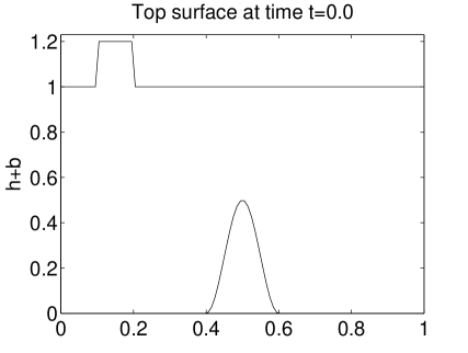
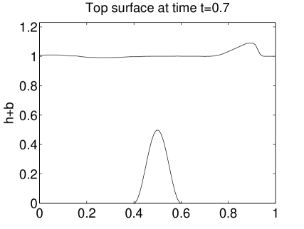
Figure 2: Propagation of small perturbations, $\varepsilon=0.2$.

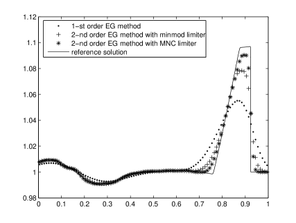
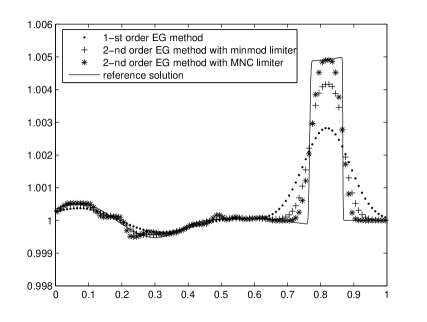
Figure 3: Propagation of small perturbations, magnified view; $\varepsilon=0.2$ (left) and $\varepsilon=0.01$ (right).

In Figure 2 the typical propagation of small height perturbations is shown at time $t=0.7$. The solution is computed on a mesh with $100\times 5$ cells and the height of the initial perturbation was $\varepsilon=0.2$. The initial disturbance generates two waves, the left-going wave runs out of the computational domain, and the right-going wave passes the bottom elevation obstacle. It is known that if the perturbations are relatively large in comparison to the discretization error a “naive” approximation of the source term, i.e. not well-balanced scheme, e.g. the fractional step method, can still yield reasonable approximations. However, for small perturbations, i.e. $\varepsilon$ of order of the discretization errors, such a scheme would yield strong oscillations over the bottom hump and the wave of interest will be lost in the noise, see [20].

In Figure 3 we compare results for water depth $h$ at time $t=0.7$ obtained by the first and second order FVEG methods using the minmod limiter and the monotonized centered limiter (denoted as MNC), respectively. In the left picture $\varepsilon=0.2$, the right picture shows results for $\varepsilon=0.01.$ The reference solutions was obtained by the second order FVEG method with the minmod limiter on a mesh with 10000 cells. For the first order scheme and the second order scheme with minmod limiter we can notice correct resolution of small perturbations of the stationary steady state even if the perturbation is of the order of the truncation error. The MNC limiter resolves the peak much more sharply, but overcompress the left-going wave. This is a well-known feature of compressive limiters, see e.g. the discussion in [33, 21, 18].

5.2 Two-dimensional quasi-stationary problem

The second example is a two-dimensional analogue of the previous one. The bottom topography is given by the function

$$b(x,y) = 0.8\,\mathrm{exp}\left(-5\left(x-0.9\right)^{2}-50\left(y-0.5\right)^{2}\right)$$ (5.58)

and the initial data are

$$h(x,y,0) = \left\{\begin{array}[]{ll}1-b(x,y)+\varepsilon&\mathrm{if}\ 0.05<x<0.15\\ 1-b(x,y)&\mathrm{otherwise}\end{array}\right.$$ (5.61)

$$u(x,y,0) = v(x,y,0)=0.$$ (5.62)

The parameter $\varepsilon$ is set to $0$ and $0.01$. The computational domain is $[0,2]\times[0,1]$ and the absorbing extrapolation boundary condition are used.

First, we take $\varepsilon=0$ and test the preservation of a two-dimensional lake at rest on a mesh with $20\times 20$ mesh cells, see Table 2. Analogously to the one-dimensional case this steady state is preserved up to the machine accuracy. In the Figure 4 we present two solutions of a perturbed problem, $\varepsilon=0.01$, which are computed on a $200\times 100$ grid (left) and on a $600\times 300$ grid (right) by the second order FVEG scheme with the minmod limiter. Notice that the FVEG method correctly approximates small perturbed waves, the perturbation propagates over the bottom hump without any oscillations. Note that the wave speed is slower over the hump, which leads to a distortion of the initially planar perturbation. The perturbed wave runs out of the computational domain and the flat surface is obtained at the end. Our results are in a good agreement with other results presented in literature, cf., e.g., [17, 20, 31, 34].

Table 2: The $L^{1}$-error of the well-balance FVEG scheme using $20\times 20$ mesh cells.

Method	$t=0.2$	$t=1$	$t=10$
first order FVEG	$2.35\times 10^{-17}$	$5.09\times 10^{-17}$	$5.02\times 10^{-17}$
second order FVEG	$4.97\times 10^{-17}$	$6.74\times 10^{-17}$	$1.53\times 10^{-16}$

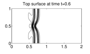
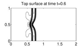
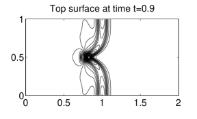
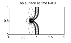
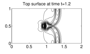
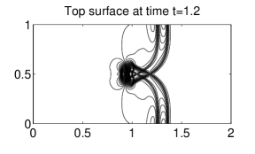
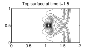
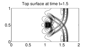
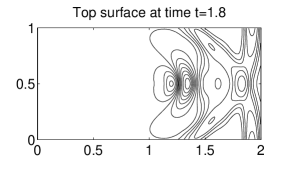
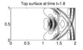
Figure 4: Two dimensional quasi-stationary problem (5.58), (5.62).

5.3 Steady jet in the rotational frame

This is a classical Rossby adjustment of an unbalanced jet in an open domain, see e.g. [5]. The initial data are a rest state superimposed by a one-dimensioal jet,

$$h(x,y,0)=1.0,\quad u(x,y,0)=0,\quad v(x,y,0)=2N_{L}(x),$$

where the shape of the velocity $v$ is given by a smooth profile

$$N_{L}(x)=\frac{(1+tanh(4x/L+2))\,(1-tanh(4x/L-2))}{(1+tanh(2))^{2}}$$

with $L=2$. We have used flat bottom topography $b(x)=0$, the parameter of the Coriolis forces $f$ and the gravitational acceleration $g$ are set to 1. The nondimensional parameter representing the effects of Coriolis forces, the Rossby number $Ro=\frac{|v(x,y,0)|}{fL}=1$ and the Burgers number reflecting the nonlinear effects is $Bu=\frac{g|h(x,y,0)|}{f^{2}L^{2}}=0.25.$ The initial jet adjusts a momentum unbalance, which emits the waves, the so-called gravity waves, propagating out from the jet. The formation of shocks can be noticed within the jet core approximately at $\pi/f,$ which is a half of a natural time scale $T_{f}=2\pi/f$, see Figure 5, 6. As time is evolved the solution tends to the equilibrium state $fv=gh_{x}$, which is a geostrophic balance as demonstrated in Figure 7. We can notice that even for long time simulations there are still small oscillations around the geostrophic equilibrium. As pointed out by Bouchut et al. [5] some wave modes with the frequencies close to $f$ remain for a longer time in the core of the jet. Their analysis for a linearized situation shows that they correspond to the gravity wave modes having almost zero group velocity, and thus are almost not propagating. For another extensive study of the stability of jets, which gives interesting eigenfunctions similar to those in Figure 5 we refer to [11].

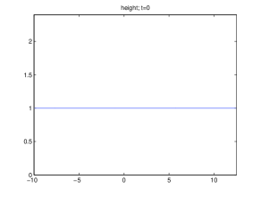
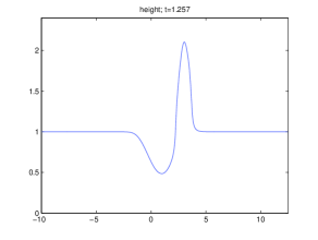
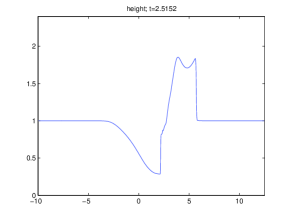
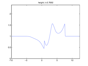
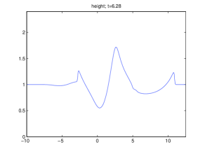
Figure 5: One-dimensional Rossby adjustment problem, time evolution of water height.

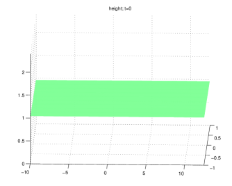
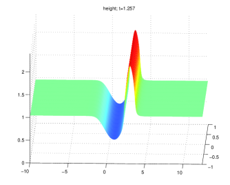
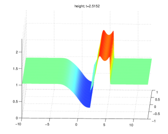
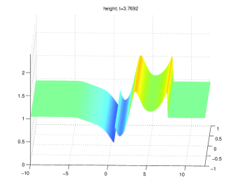
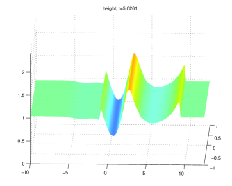
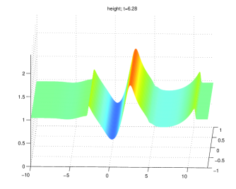
Figure 6: Rossby adjustment problem, time evolution of water height, two-dimensional graphs.

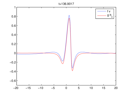
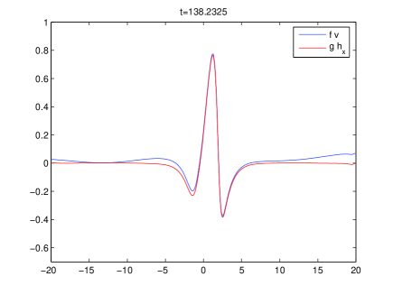
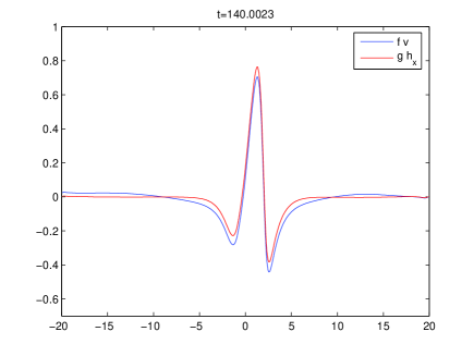
Figure 7: One-dimensional Rossby adjustment problem at different times, geostrophic balance.

5.4 Accuracy and performance

In this experiment we compare accuracy and computational time of the well-balanced FVEG, the second order well-balanced FV method of Audusse et al. [2] and its fourth order extension due to Noelle et al. [31]. We choose a fully two-dimensional experiment analogous to that of Xing and Shu [34], but include moreover the effect of Coriolis forces by setting $f=10$. The gravitational constant was set to $g=9.812.$ The bottom topography and the initial data are given as follows

$$b(x,y) = \sin(2\pi x)+\cos(2\pi y),$$

$$h(x,y,0) = 10+\mbox{exp}({\sin(2\pi x)})\cos(2\pi y),$$

$$hu(x,y,0) = \sin(\cos(2\pi x))\sin(2\pi y),$$

$$hv(x,y,0) = \cos(2\pi x)\cos(\sin(2\pi y)).$$

The computational domain $[0,1]\times[0,1]$ was consecutively divided into $25$, $50,\dots,800$ mesh cells in each direction. We have compared solutions obtained by the second order FVEG scheme as well as by the second order and fourth order well-balanced FVM at time $T=0.05$. For the second order well-balanced FVM of Audusse et al. the second order Runge-Kutta method was used for time integration, the third order Gaussian quadrature was used for cell-interface integrals of fluxes and the second order WENO recovery was applied. The reference solution was obtained by the fourth order well-balanced FV method of Noelle et al. [31].

Tables 3 and 4 contain the $L^{1}$ errors and experimental order of convergence (EOC) for the FVEG for both CFL numbers 0.8 as well as 0.5, respectively. The well-balanced higher order directional splitting FVM is in general stable up to CFL=0.5. The $L^{1}$ errors for its second order version are presented in Table 5. We can indeed see that both methods are second order accurate in all components. Moreover, the second order FVEG scheme is almost 10 times more accurate than the second order FVM, see Table 5 as well as the left picture of the Figure 8.

Figure 8 illustrates the CPU/accuracy behaviour graphically. We use the logarithmic scale on $x-,y-$ axis. On the $y-$ axis the $L^{1}$ errors in first component $h$ is depicted. Errors in other components yield analogous results. On the left of Figure 8 a comparison between second order FVEG and FV methods are presented, whereas on the right we show the comparison between the fourth order well-balanced FVM of Noelle [31] and the second order FVEG scheme. The FVEG schemes yields on coarse meshes still more accurate solutions. In fact, for meshes up to approximately $100\times 100$ cells, which are actually often used for practical computations, it is more efficient to use the second order FVEG scheme than the fourth order FVM. The superiority of the fourth order scheme is showing up on fine grids, see the right graph of Figure 8.

We should point out that no attempt has been made in order to optimize the codes with respect to their CPU performance. Our extensive numerical treatment indicates that both well-balanced second order methods, the FVEG as well as the FVM are actually comparable with respect to their computational time.

Table 3: FVEG scheme: Convergence in the $L^{1}$ norm, CFL=0.8

N	$L^{1}$ error in $h$	EOC	$L^{1}$ error in $hu$	EOC	$L^{1}$ error in $hv$	EOC
25	1.04e-02		3.56e-02		8.52e-02
50	2.42e-03	2.10	8.71e-03	2.03	2.15e-02	1.99
100	6.01e-04	2.01	2.23e-03	1.96	5.50e-03	1.96
200	1.54e-04	1.96	5.76e-04	1.95	1.44e-03	1.93
400	3.97e-05	1.96	1.47e-04	1.97	3.69e-04	1.96
800	1.02e-05	1.97	3.71e-05	1.98	9.40e-05	1.97

Table 4: FVEG scheme: Convergence in the $L^{1}$ norm, CFL=0.5

N	$L^{1}$ error in $h$	EOC	$L^{1}$ error in $hu$	EOC	$L^{1}$ error in $hv$	EOC
25	1.37e-02		6.19e-02		1.18e-01
50	2.80e-03	2.29	1.05e-02	2.56	2.33e-02	2.34
100	5.23e-04	2.42	1.80e-03	2.54	4.25e-03	2.45
200	1.04e-04	2.33	3.63e-04	2.31	8.12e-04	2.39
400	2.45e-05	2.09	8.79e-05	2.05	1.80e-04	2.17
800	6.14e-06	1.99	2.20e-05	2.00	4.36e-05	2.04

Table 5: FV scheme: Convergence in the $L^{1}$ norm, CFL=0.5

N	$L^{1}$ error in $h$	EOC	$L^{1}$ error in $hu$	EOC	$L^{1}$ error in $hv$	EOC
25	4.53e-02		2.13e-01		3.40e-01
50	1.32e-02	1.77	5.57e-02	1.94	9.51e-02	1.84
100	3.50e-03	1.92	1.42e-02	1.97	2.52e-02	1.92
200	8.95e-04	1.97	3.58e-03	1.99	6.46e-03	1.96
400	2.26e-04	1.99	8.96e-04	2.00	1.63e-03	1.99
800	5.67e-05	1.99	2.24e-04	2.00	4.10e-04	1.99

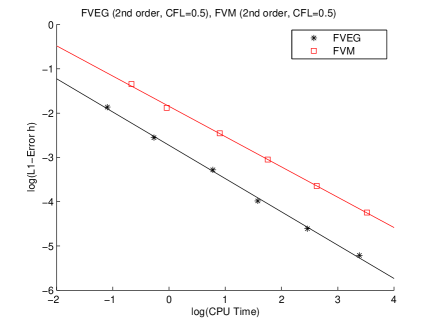
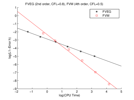
Figure 8: Efficiency test: $L^{1}$ error over the CPU time; the second order FVEG and second order FV schemes (left) as well as the fourth order FVM and the second order FVEG scheme (right).

6 Conclusions

In the present paper we have developed a new well-balanced scheme within the framework of the finite volume evolution Galerkin (FVEG) scheme. The scheme is applied for the shallow water equations with source terms modelling the bottom topography and the Coriolis forces. The key ingredient of this FVEG scheme is a new well-balanced approximate representation of the solution, cf. Lemma 3.2, which together with a recent quadrature rule from [27] leads to the multidimensional approximate evolution operators (3.43), (3.44). These approximate evolution operators are used in a predictor step. In fact we are predicting the solution at cell interfaces and do not need to use the hydrostatic reconstruction as it is done by Audusse at el. [2].

In the following correction step, which is the finite volume update step, the source term is approximated in the interface-based way. We have proved that the lake at rest, the steady jet in the rotational frame as well as their combinations are preserved, cf. Theorems 2.1 and 3.1. Numerical experiments in one and two space dimensions demonstrate correct resolution of these equilibrium states and of their small perturbations. For smooth solutions the accuracy of the well-balanced FVEG scheme is superior to that of a recent FV scheme while the CPU time is comparable.

In future work we want to extend our well-balanced schemes to shallow water equations with nonlinear friction, which appears in oceanographic as well as river flow modelling. Another challenge is presented by multi-layere shallow water models, which are important in oceanology, meteorology and climatology.

Acknowledgements
This research was supported by the Graduate Colleges ‘Conservation principles in the modelling and simulation of marine, atmospherical and technical systems’ and ‘Hierarchie and Symmetry in Mathematical Systems’ both sponsored by the Deutsche Forschungsgemeinschaft, and by the EU-Network Hyke HPRN-CT-2002-00282. The authors gratefully acknowledge these supports. Furthermore, we would like to thank Normann Pankratz, RWTH Aachen, for fruitful discussions and for providing the FV results [2, 31] used in the comparisons in Section 5.4.

Appendix A Derivation of the exact integral equations

Applying theory of bicharacteristics to (3.2) we can derive exact integral equations in an analogous way as in [27]. In order to keep the presentation self-contained we briefly rewrite main steps of the derivation.

Let $R$ be the matrix of right eigenvectors corresponding to direction $\mbox{\boldmath$n$}:=(\cos(\theta),\sin(\theta))$. Its inverse reads

$$\mbox{\boldmath$R$}^{-1}=\frac{1}{2}\left(\begin{array}[]{ccc}-1&\frac{\tilde{c}}{g}\cos\theta&\frac{\tilde{c}}{g}\sin\theta\\ 0&2\sin\theta&-2\cos\theta\\ 1&\frac{\tilde{c}}{g}\cos\theta&\frac{\tilde{c}}{g}\sin\theta\\ \end{array}\right).$$

Let us define the vector of characteristic variables $v$ by

$$\mbox{\boldmath$v$}:=\mbox{\boldmath$R$}^{-1}\mbox{\boldmath$w$}.$$

Multiplying system (3.2) by $\mbox{\boldmath$R$}^{-1}$ from the left yields the following characteristic system

$$\frac{\partial\mbox{\boldmath$v$}}{\partial t}+\mbox{\boldmath$B$}_{1}(\tilde{\mbox{\boldmath$v$}})\frac{\partial\mbox{\boldmath$v$}}{\partial x}+\mbox{\boldmath$B$}_{2}(\tilde{\mbox{\boldmath$v$}})\frac{\partial\mbox{\boldmath$v$}}{\partial y}=\mbox{\boldmath$r$},$$

where

$$\mbox{\boldmath$B$}_{1} = \displaystyle\left(\begin{array}[]{ccc}\tilde{u}-\tilde{c}\cos\theta&-\frac{1}{2}\,\tilde{h}\sin\theta&0\\ -g\sin\theta&\tilde{u}&g\sin\theta\\ 0&\frac{1}{2}\,\tilde{h}\sin\theta&\tilde{u}+\tilde{c}\cos\theta\\ \end{array}\right),$$ (A.66)

$$\mbox{\boldmath$B$}_{2} = \displaystyle\left(\begin{array}[]{ccc}\tilde{v}-\tilde{c}\sin\theta&\frac{1}{2}\,\tilde{h}\cos\theta&0\\ g\cos\theta&\tilde{v}&-g\cos\theta\\ 0&-\frac{1}{2}\,\tilde{h}\cos\theta&\tilde{v}+\tilde{c}\sin\theta\\ \end{array}\right),$$ (A.70)

$$\mbox{\boldmath$r$}(\mbox{\boldmath$n$}) = \left(\begin{array}[]{c}r_{1}\\ r_{2}\\ r_{3}\\ \end{array}\right)=\mbox{\boldmath$R$}^{-1}(\mbox{\boldmath$n$})\mbox{\boldmath$t$}=\left(\begin{array}[]{c}\frac{1}{2}\frac{\tilde{c}}{g}((-gb_{x}+fv)\cos\theta-(gb_{y}+fu)\sin\theta)\\ (-gb_{x}+fv)\sin\theta+(gb_{y}+fu)\cos\theta\\ \frac{1}{2}\frac{\tilde{c}}{g}((-gb_{x}+fv)\cos\theta-(gb_{y}+fu)\sin\theta)\\ \end{array}\right)$$ (A.77)

(A.78)

and the characteristic variables $v$ are

$$\mbox{\boldmath$v$}(\mbox{\boldmath$n$})=\left(\begin{array}[]{c}v_{1}\\ v_{2}\\ v_{3}\\ \end{array}\right)=\mbox{\boldmath$R$}^{-1}(\mbox{\boldmath$n$})\mbox{\boldmath$u$}=\left(\begin{array}[]{c}\frac{1}{2}(-h+\frac{\tilde{c}}{g}u\cos\theta+\frac{\tilde{c}}{g}v\sin\theta)\\ u\sin\theta-v\cos\theta\\ \frac{1}{2}(h+\frac{\tilde{c}}{g}u\cos\theta+\frac{\tilde{c}}{g}v\sin\theta)\\ \end{array}\right).$$

The quasi-diagonalised system of the linearized shallow water equations has the following form

$$\frac{\partial\mbox{\boldmath$v$}}{\partial t}+\left(\begin{array}[]{ccc}\tilde{u}-\tilde{c}\cos\theta&0&0\\ 0&\tilde{u}&0\\ 0&0&\tilde{u}+\tilde{c}\cos\theta\\ \end{array}\right)\frac{\partial\mbox{\boldmath$v$}}{\partial x}+\left(\begin{array}[]{ccc}\tilde{v}-\tilde{c}\sin\theta&0&0\\ 0&\tilde{v}&0\\ 0&0&\tilde{v}+\tilde{c}\sin\theta\\ \end{array}\right)\frac{\partial\mbox{\boldmath$v$}}{\partial y}=\mbox{\boldmath$s$}+\mbox{\boldmath$r$}$$ (A.79)

with

$$\mbox{\boldmath$s$}=\left(\begin{array}[]{c}s_{1}\\ s_{2}\\ s_{3}\\ \end{array}\right)=\left(\begin{array}[]{c}\frac{1}{2}\tilde{h}(\sin\theta\frac{\partial v_{2}}{\partial x}+\cos\theta\frac{\partial v_{2}}{\partial y})\\ g\sin\theta(\frac{\partial v_{1}}{\partial x}-\frac{\partial v_{3}}{\partial x})-g\cos\theta(\frac{\partial v_{1}}{\partial y}-\frac{\partial v_{3}}{\partial y})\\ \frac{1}{2}\tilde{h}(\cos\theta\frac{\partial v_{2}}{\partial x}-\sin\theta\frac{\partial v_{2}}{\partial y})\\ \end{array}\right).$$

Let us denote by $\mbox{\boldmath$x$}_{\ell}$ the $\ell$-th bicharacteristic corresponding to the $\ell$-th equation of system (A.79). The bicharacteristic $\mbox{\boldmath$x$}_{\ell}$ is defined in the following way

$$\frac{d\mbox{\boldmath$x$}_{\ell}(s)}{ds}=\left(\begin{array}[]{rr}b^{1}_{\ell\ell}\\ b^{2}_{\ell\ell}\end{array}\right),$$

where $b^{1}_{\ell\ell},b^{2}_{\ell\ell}$ are the diagonal entries of the matrices $\mbox{\boldmath$B$}_{1},\mbox{\boldmath$B$}_{2}$, respectively. The bicharacteristics $\mbox{\boldmath$x$}_{\ell}$ create the surface of the so-called bicharacteristic cone, see Fig. 1, with the apex $P=(x,y,t_{n}+\tau)$ and the footpoints

$$Q_{1}(\theta) = (x-(\tilde{u}-\tilde{c}\cos\theta)\tau,y-(\tilde{v}-\tilde{c}\sin\theta)\tau,t_{n}),$$

$$Q_{2} \equiv Q_{0}=(x-\tilde{u}\tau,y-\tilde{v}\tau,t_{n}),$$

$$Q_{3}(\theta) = (x-(\tilde{u}+\tilde{c}\cos\theta)\tau,y-(\tilde{v}+\tilde{c}\sin\theta)\tau,t_{n}).$$

Remember that $\tau=\Delta t/2$ in our case. Integrating each equation of (A.79) along the corresponding bicharacteristic from the apex $P$ down to the footpoints $Q_{\ell}$ we get

$$v_{\ell}(P)=v_{\ell}(Q_{\ell})+\int_{t_{n}}^{t_{n}+\tau}s_{\ell}(Q_{\ell}(\tilde{t}))+r_{\ell}(Q_{\ell}(\tilde{t}))\mbox{d}\tilde{t},\quad\ell=1,2,3.$$ (A.80)

Now multiplying (A.80) with $R$ from the left and averaging over all directions we go back to the original variables $w$

$$\mbox{\boldmath$w$}(P)=$$

$$\frac{1}{2\pi}\int_{0}^{2\pi}\left(\begin{array}[]{c}-v_{1}(Q_{1}(\theta),\theta)+v_{3}(Q_{3}(\theta),\theta)\\ \frac{g}{\tilde{c}}\cos\theta v_{1}(Q_{1}(\theta),\theta)+\sin\theta v_{2}(Q_{2}(\theta),\theta)+\frac{g}{\tilde{c}}\cos\theta v_{3}(Q_{3}(\theta),\theta))\\ \frac{g}{\tilde{c}}\sin\theta v_{1}(Q_{1}(\theta),\theta)-\cos\theta v_{2}(Q_{2}(\theta),\theta)+\frac{g}{\tilde{c}}\sin\theta v_{3}(Q_{3}(\theta),\theta))\\ \end{array}\right)\mbox{d}\theta$$ (A.84)

$$+\frac{1}{2\pi}\int_{0}^{2\pi}\left(\begin{array}[]{c}-s_{1}^{{}^{\prime}}(\theta)-r_{1}^{{}^{\prime}}(\theta)+s_{3}^{{}^{\prime}}(\theta)+r_{3}^{{}^{\prime}}(\theta)\\ \frac{g}{\tilde{c}}\cos\theta(s_{1}^{{}^{\prime}}(\theta)+r_{1}^{{}^{\prime}}(\theta))+\sin\theta(s_{2}^{{}^{\prime}}(\theta)+r_{2}^{{}^{\prime}}(\theta))+\frac{g}{\tilde{c}}\cos\theta(s_{3}^{{}^{\prime}}(\theta)+r_{3}^{{}^{\prime}}(\theta))\\ \frac{g}{\tilde{c}}\sin\theta(s_{1}^{{}^{\prime}}(\theta)+r_{1}^{{}^{\prime}}(\theta))-\cos\theta(s_{2}^{{}^{\prime}}(\theta)+r_{2}^{{}^{\prime}}(\theta)+\frac{g}{\tilde{c}}\sin\theta(s_{3}^{{}^{\prime}}(\theta)+r_{3}^{{}^{\prime}}(\theta))\\ \end{array}\right)\mbox{d}\theta,$$ (A.88)

where $s_{\ell}^{{}^{\prime}}(\theta)=\int_{t_{n}}^{t_{n}+\tau}{s_{\ell}(\mbox{\boldmath$x$}_{\ell}(\tilde{t},\theta),\tilde{t},\theta)\mbox{d}\tilde{t}}$ is an integral along the $\ell$-th bicharacteric and the analogous notation holds for source terms $r_{\ell}$. It should be noted that the source term $s_{\ell}$ in (A.80) arrives from to the multidimensionality of the system, whereas the source term $r_{\ell}$ is a physical source term.

Now, we have $\lambda_{1}=-\lambda_{3}$, $Q_{1}(\theta+\pi)=Q_{3}(\theta)$ and the characteristic variables $v_{\ell}$ are $2\pi$-periodic. Applying the Gauss integration, cf. (3.38), in order to avoid the derivatives of dependent variables appearing in $s$ we can, after analogous computations as in [23, 27], reformulate the exact integral equations (A) in the following way

$$h\left(P\right) = \frac{1}{2\pi}\int_{0}^{2\pi}h\left(Q\right)-\frac{\tilde{c}}{g}u\left(Q\right)\cos\theta-\frac{\tilde{c}}{g}v\left(Q\right)\sin\theta\mbox{d}\theta\phantom{mmmmmmmmmmmmmmmm}$$

$$-\frac{1}{2\pi}\int_{t_{n}}^{t_{n}+\tau}\frac{1}{t_{n}+\tau-\tilde{t}}\int_{0}^{2\pi}\frac{\tilde{c}}{g}\left(u(\tilde{Q})\cos\theta+v(\tilde{Q})\sin\theta\right)\mbox{d}\theta\mbox{d}\tilde{t}$$

$$+\frac{1}{2\pi}\tilde{c}\int_{t_{n}}^{t_{n}+\tau}\int_{0}^{2\pi}\left(b_{x}(\tilde{Q})\cos\theta+b_{y}(\tilde{Q})\sin\theta\right)\mbox{d}\theta\mbox{d}\tilde{t}$$

$$-\frac{1}{2\pi}\frac{\tilde{c}f}{g}\int_{t_{n}}^{t_{n}+\tau}\int_{0}^{2\pi}\left(v(\tilde{Q})\cos\theta-u(\tilde{Q})\sin\theta\right)\mbox{d}\theta\mbox{d}\tilde{t},$$

$$u\left(P\right) = \frac{1}{2}u\left(Q_{0}\right)+\frac{1}{2\pi}\int_{0}^{2\pi}-\frac{g}{\tilde{c}}h\left(Q\right)\cos\theta+u\left(Q\right)\cos^{2}\theta+v\left(Q\right)\sin\theta\cos\theta\,\mbox{d}\theta$$

$$-\frac{g}{2}\int_{t_{n}}^{t_{n}+\tau}\left(h_{x}(\tilde{Q}_{0})+b_{x}(\tilde{Q}_{0})\right)\mbox{d}\tilde{t}$$

$$-\frac{g}{2\pi}\int_{t_{n}}^{t_{n}+\tau}\int_{0}^{2\pi}\left(b_{x}(\tilde{Q})\cos^{2}\theta+b_{y}(\tilde{Q})\sin\theta\cos\theta\right)\mbox{d}\theta\mbox{d}\tilde{t}$$

$$+\frac{1}{2\pi}\int_{t_{n}}^{t_{n}+\tau}\frac{1}{t_{n}+\tau-\tilde{t}}\int_{0}^{2\pi}\left(u(\tilde{Q})\cos 2\theta+v(\tilde{Q})\sin 2\theta\right)\mbox{d}\theta\mbox{d}\tilde{t}$$

$$+\frac{f}{2}\int_{t_{n}}^{t_{n}+\tau}v(\tilde{Q}_{0})\mbox{d}\tilde{t}+\frac{f}{2\pi}\int_{t_{n}}^{t_{n}+\tau}\int_{0}^{2\pi}\left(v(\tilde{Q})\cos^{2}\theta-u(\tilde{Q})\sin\theta\cos\theta\right)\mbox{d}\theta\mbox{d}\tilde{t},$$

$$v\left(P\right) = \frac{1}{2}v\left(Q_{0}\right)+\frac{1}{2\pi}\int_{0}^{2\pi}-\frac{g}{\tilde{c}}h\left(Q\right)\sin\theta+u\left(Q\right)\sin\theta\cos\theta+v\left(Q\right)\sin^{2}\theta\,\mbox{d}\theta$$

$$-\frac{g}{2}\int_{t_{n}}^{t_{n}+\tau}\left(h_{y}(\tilde{Q}_{0})+b_{y}(\tilde{Q}_{0})\right)\mbox{d}\tilde{t}$$

$$-\frac{g}{2\pi}\int_{t_{n}}^{t_{n}+\tau}\int_{0}^{2\pi}\left(b_{x}(\tilde{Q})\sin\theta\cos\theta+b_{y}(\tilde{Q})\sin^{2}\theta\right)\mbox{d}\theta\mbox{d}\tilde{t}$$

$$+\frac{1}{2\pi}\int_{t_{n}}^{t_{n}+\tau}\frac{1}{t_{n}+\tau-\tilde{t}}\int_{0}^{2\pi}\left(u(\tilde{Q})\sin 2\theta-v(\tilde{Q})\cos 2\theta\right)\mbox{d}\theta\mbox{d}\tilde{t}$$

$$-\frac{f}{2}\int_{t_{n}}^{t_{n}+\tau}u(\tilde{Q}_{0})\mbox{d}\tilde{t}+\frac{f}{2\pi}\int_{t_{n}}^{t_{n}+\tau}\int_{0}^{2\pi}\left(v(\tilde{Q})\sin\theta\cos\theta-u(\tilde{Q})\sin^{2}\theta\right)\mbox{d}\theta\mbox{d}\tilde{t}.$$

Recall that $\tilde{Q}_{0}=(x-\tilde{u}(t_{n}+\tau-\tilde{t}),y-\tilde{v}(t_{n}+\tau-\tilde{t}),\tilde{t})$, $\tilde{Q}=(x-\tilde{u}(t_{n}+\tau-\tilde{t})+c(t_{n}+\tau-\tilde{t})\cos\theta,y-\tilde{v}(t_{n}+\tau-\tilde{t})+c(t_{n}+\tau-\tilde{t})\sin\theta,\tilde{t})$ stays for an arbitrary point on the mantle and $Q=Q(\tilde{t})\Big{|}_{\tilde{t}=t_{n}}$ denotes a point at the perimeter of the sonic circle at time $t_{n}.$

Appendix B Proof of Lemma 3.2

Proof.

We show here that the approximate integral equations (3.2)-(3.2) are consistent with the exact integral equations (3.1)-(3.1), i.e. (A)-(A). In (3.1) the integral with bottom topography terms can be rewritten using the polar-type transformation along the mantle of the bicharacteristic cone, i.e. $x_{\tilde{Q}}=x+r(\cos\theta-\frac{\tilde{u}}{\tilde{c}}),\,y_{\tilde{Q}}=y+r(\sin\theta-\frac{\tilde{v}}{\tilde{c}})$, where $r=\tilde{c}(t_{n}+\tau-\tilde{t})$ is the circle radius at the time level $\tilde{t}\in[t_{n},t_{n}+\tau].$ Thus, we have

$$\frac{db}{dr}(r,\theta)=b_{x}(x_{\tilde{Q}},y_{\tilde{Q}})\cos\theta+b_{y}(x_{\tilde{Q}},y_{\tilde{Q}})\sin\theta-\frac{1}{\tilde{c}}\left(\tilde{u}b_{x}(x_{\tilde{Q}},y_{\tilde{Q}})+\tilde{v}b_{y}(x_{\tilde{Q}},y_{\tilde{Q}})\right).$$

Therefore,

$$\frac{\tilde{c}}{2\pi}\int_{t_{n}}^{t_{n}+\tau}\int_{0}^{2\pi}\left(b_{x}(\tilde{Q})\cos\theta+b_{y}(\tilde{Q})\sin\theta\right)\mbox{d}\theta\mbox{d}\tilde{t}$$ (B.93)

$$=\frac{\tilde{c}}{2\pi}\int_{\tilde{c}\tau}^{0}\int_{0}^{2\pi}\frac{\mbox{d}b(r,\theta)}{\mbox{d}r}\mbox{d}\theta(-\frac{\mbox{d}r}{\tilde{c}})+\frac{1}{2\pi}\int_{t_{n}}^{t_{n}+\tau}\int_{0}^{2\pi}\tilde{u}b_{x}(\tilde{Q})+\tilde{v}b_{y}(\tilde{Q})\mbox{d}\theta\mbox{d}\tilde{t}$$

$$=\int_{0}^{\tilde{c}\tau}\frac{\mbox{d}}{\mbox{d}r}\left(\frac{1}{2\pi}\int_{0}^{2\pi}b\,\mbox{d}\theta\right)\mbox{d}r+\frac{1}{2\pi}\int_{t_{n}}^{t_{n}+\tau}\int_{0}^{2\pi}\tilde{u}b_{x}(\tilde{Q})+\tilde{v}b_{y}(\tilde{Q})\mbox{d}\theta\mbox{d}\tilde{t}$$

$$=\frac{1}{2\pi}\int_{0}^{2\pi}b(Q)\mbox{d}\theta-b(P)+\frac{1}{2\pi}\int_{t_{n}}^{t_{n}+\tau}\int_{0}^{2\pi}\tilde{u}b_{x}(\tilde{Q})+\tilde{v}b_{y}(\tilde{Q})\mbox{d}\theta\mbox{d}\tilde{t},$$

which yields the corresponding terms in (3.2).

Further, we show that the integrals in (3.1) containing the Coriolis forces are of order ${\mathcal{O}}(\Delta t^{2})$; note that $\tau=\Delta t/2$. Applying the rectangle rule in time and the Taylor expansion from Lemma 3.1 in the center of the sonic circle $Q_{0}$ yields

$$\int_{t_{n}}^{t_{n}+\tau}\int_{0}^{2\pi}v(\tilde{Q})\cos\theta\mbox{d}\theta\mbox{d}\tilde{t}=\tau\int_{0}^{2\pi}v(Q)\cos\theta\mbox{d}\theta$$ (B.94)

$$= \tau\int_{0}^{2\pi}(v(Q_{0})\cos\theta+c\tau\,v_{x}(Q_{0})\cos^{2}\theta+c\tau\,v_{y}(Q_{0})\cos\theta\sin\theta+O(\Delta t^{2}))\mbox{d}\theta$$

$$= {\mathcal{O}}(\Delta t^{2})$$

with an analogous approximation for the Coriolis forces in $y$-direction. Together with (B.93) and (B.94) this yields the approximate integral equation (3.2).

In the equation (3.1) for velocity $u$ we apply for the mantle integrals containing the bottom elevation terms the rectangle rule in time and the Taylor expansion over the center $Q_{0}$ of the sonic circle $S_{0}$ at time $t_{n}$, which lead to

$$\frac{1}{2\pi}g\int\limits_{t_{n}}^{t_{n}+\tau}\int\limits_{0}^{2\pi}\left(b_{x}(\tilde{Q})\cos\theta+b_{y}(\tilde{Q})\sin\theta\right)\cos\theta\ \mbox{d}\theta\,\mbox{d}\tilde{t}=\frac{g\tau}{2}b_{x}(Q_{0})+{\mathcal{O}}(\Delta t^{2}).$$ (B.95)

To complete we eliminate the derivative by replacing the term $b_{x}(Q_{0})$ by its average over the sonic circle $S_{0}$ and applying the Gauss theorem

$$b_{x}(Q_{0})=\frac{1}{\pi\tilde{c}^{2}\Delta{t}^{2}}\int_{S_{0}}b_{x}(Q)\,\mbox{d}x\mbox{d}y+O(\Delta t^{2})=\frac{1}{\pi\tilde{c}\tau}\int_{0}^{2\pi}b(Q)\cos\theta\,\mbox{d}\theta+{\mathcal{O}}(\Delta t^{2}),$$ (B.96)

which after substitution into (B.95) yields

$$\frac{1}{2\pi}g\int\limits_{t_{n}}^{t_{n}+\tau}\int\limits_{0}^{2\pi}\left(b_{x}(\tilde{Q})\cos\theta+b_{y}(\tilde{Q})\sin\theta\right)\cos\theta\ \mbox{d}\theta\,\mbox{d}\tilde{t}=\frac{g}{\tilde{c}}\frac{1}{2\pi}\int_{0}^{2\pi}b(Q)\cos\theta\,\mbox{d}\theta+{\mathcal{O}}(\Delta t^{2}).$$ (B.97)

Rewriting the Coriolis forces terms using their primitives we obtain analogously to (B.95) and (B.96)

$$\frac{f}{2\pi}\int_{t_{n}}^{t_{n}+\tau}\int_{0}^{2\pi}\left(v(\tilde{Q})\cos^{2}\theta-u(\tilde{Q})\sin\theta\cos\theta\right)\mbox{d}\theta\mbox{d}\tilde{t}$$ (B.98)

$$=\frac{g}{2\pi}\int_{t_{n}}^{t_{n}+\tau}\int_{0}^{2\pi}\left(V_{x}(\tilde{Q})\cos\theta-U_{y}(\tilde{Q})\sin\theta\right)\cos\theta\ \mbox{d}\theta\,\mbox{d}\tilde{t}$$

$$=\frac{g}{\tilde{c}}\frac{1}{2\pi}\int_{0}^{2\pi}V(Q)\cos\theta\,\mbox{d}\theta+{\mathcal{O}}(\Delta t^{2}).$$

This balances together with (B.97) the analogous term with $h(Q)\cos\theta$ in (3.1). The integral along the middle bicharacteristic

$$\frac{g}{2}\int_{t_{n}}^{t_{n}+\tau}\left(h_{x}(\tilde{Q}_{0})+b_{x}(\tilde{Q}_{0})-\frac{f}{g}v(\tilde{Q}_{0})\right)\,\mbox{d}\tilde{t}=\frac{g}{2}\int_{t_{n}}^{t_{n}+\tau}\left(h_{x}(\tilde{Q}_{0})+b_{x}(\tilde{Q}_{0})-V_{x}(\tilde{Q}_{0})\right)\,\mbox{d}\tilde{t}$$

can be approximated in a similar way as (B.96) applying the Gauss theorem at each intermediate circular section at $\tilde{t}$ along the mantle of the bicharacteristic cone. Substituting into (3.1) gives (3.2). Approximation (3.2) for the velocity $v$ is obtained in an analogous way as (3.2). mm

References

- [1] Abgrall R, Mezine M. Construction of second order accurate monotone and stable residual distribution schemes for unsteady flow problems. J. Comput. Phys. 2003; 188(1):16-55.
- [2] Audusse E, Bouchut F, Bristeau M-O, Klein R, Perthame B. A fast and stable well-balanced scheme with hydrostatic reconstruction for shallow water flows. SIAM J. Sci. Comp. 2004; 25:205-206.
- [3] Billet S, Toro E.F. On WAF-type schemes for multidimensional hyperbolic conservation laws. J. Comput. Phys. 1997; 130:1-24.
- [4] Botta N, Klein R, Langenberg S, Lützenkirchen S. Well balanced finite volume methods for nearly hydrostatic flows. J. Comp. Phys. 2004; 196: 539-565.
- [5] Bouchut F, Le Sommer J, Zeitlin V. Frontal geostrophic adjustment and nonlinear-wave phenomena in one dimensional rotating shallow water. Part 2: high-resolution numerical simulations, to appear in J. Fluid Mech. 2004; 514:35-63.
- [6] Colella, P. Multidimensional upwind methods for hyperbolic conservation laws. J. Comput. Phys. 1990; 87:171-200.
- [7] Csík A, Ricchiuto M., Deconinck H. A conservative formulation of the multidimensional upwind residual distribution schemes for general nonlinear conservation laws. J. Comput. Phys. 2002; 179(1):286-312.
- [8] Deconinck H, Roe P, Struijs R. A multidimensional generalization of Roe’s flux difference splitter for the Euler equations. Comput. Fluids 1993; 22(2-3):215-222.
- [9] Fey M. Multidimensional upwinding, Part II. Decomposition of the Euler equations into advection equations. J. Comp. Phys. 1998; 143:181-199.
- [10] Gallouët T, Hérard J-M, Seguin N. Some approximate Godunov schemes to compute shallow-water equations wih topography, Computers and Fluids 2003; 32:479-513.
- [11] Gjevik B, Moe H, Ommundsen A. A high resolution tidal model for the area around The Lofoten Islands, northern Norway, Continental Shelf Research 2002; 22(1): 485-504.
- [12] Greenberg JM, LeRoux A-Y. A well-balanced scheme for numerical processing of source terms in hyperbolic equations, SIAM J. Numer. Anal. 1996; 33:1-16.
- [13] Jin S. A steady-state capturing method for hyperbolic systems with geometrical source terms. M2AN, Math. Model. Numer. Anal. 2001; 35(4):631-646.
- [14] Klein R. An applied mathematical view of meteorological modelling, In: Proceedings ICAM 2003, eds. J.M.Hill and R. Moore, 2003; pp. 227-270.
- [15] Kröger T, Lukáčová-Medvid’ová M. An evolution Galerkin scheme for the shallow water magnetohydro-dynamic (SMHD) equations in two space dimensions. J. Comp. Phys. 2005; 206:122-149.
- [16] Kröger T, Noelle S. On the connection between some Riemann-solver free approaches to the approximation of multi-dimensional systems of hyperbolic conservation laws. Math. Model. Numer. Anal. 2004; 38:989-1009.
- [17] Kurganov A, Levy D. Central-upwind schemes for the Saint-Venant system. M2AN, Math. Model. Numer. Anal. 2002; 36(3):397-425.
- [18] Kurganov A, Petrova G, Popov B. Adaptive semi-discrete central-upwind schemes for nonconvex hyperbolic conservation laws. accepted to SIAM J. Sci. Comp. 2006.
- [19] LeVeque RJ. Wave propagation algorithms for multi-dimensional hyperbolic systems. J. Comp. Phys. 1997; 131:327-353.
- [20] LeVeque RJ. Balancing source terms and flux gradients in high-resolution Godunov methods: The quasi-steady wave propagation algorithm. J. Comp. Phys. 1998; 146:346-365.
- [21] Lie K.-A., Noelle S. On the artificial compression method for second order non-oscillatory central difference schemes for systems of conservation laws. SIAM J. Sci. Comp. 2003; 24(4): 1157-1174.
- [22] Lukáčová-Medvid’ová M. Multidimensional bicharacteristics finite volume methods for the shallow water equations. In: Finite Volumes for Complex Applications, eds. R. Hérbin and D. Kröner, Hermes, 2002, 389-397.
- [23] Lukáčová-Medvid’ová M, Morton KW, Warnecke G. Evolution Galerkin methods for hyperbolic systems in two space dimensions. MathComp. 2000; 69:1355–1384.
- [24] Lukáčová-Medvid’ová M, Morton KW, Warnecke G. On high-resolution finite volume evolution Galerkin schemes for genuinely multidimensional hyperbolic conservation laws, In: European Congress on Computational Methods in Applied Sciences and Engineering, ECCOMAS 2000, eds. Onate et al., CIMNE 2000, 1-14.
- [25] Lukáčová-Medvid’ová M, Morton KW, Warnecke G. Finite volume evolution Galerkin methods for Euler equations of gas dynamics. Int. J. Numer. Meth. Fluids 2002; 40(3-4):425-434.
- [26] Lukáčová-Medvid’ová M, Saibertová J, Warnecke G. Finite volume evolution Galerkin methods for nonlinear hyperbolic systems. J. Comp. Phys. 2002; 183:533-562.
- [27] Lukáčová-Medvid’ová M, Morton KW, Warnecke G. Finite volume evolution Galerkin (FVEG) methods for hyperbolic problems. SIAM J. Sci. Comput. 2004; 26(1):1-30.
- [28] Lukáčová-Medvid’ová M, Warnecke G, Zahaykah Y. On the stability of the evolution Galerkin schemes applied to a two-dimensional wave equation system. accepted to SIAM J. Numer. Anal. 2006.
- [29] Lukáčová-Medvid’ová M, Warnecke G, Zahaykah Y. Finite volume evolution Galerkin schemes for three-dimensional wave equation system. submitted, 2004.
- [30] Noelle S. The MOT-ICE: a new high-resolution wave-propagation algorithm for multi-dimensional systems of conservative laws based on Fey’s method of transport. J. Comput. Phys. 2000; 164:283-334.
- [31] Noelle S, Pankratz N, Puppo G, Natvig J. Well-balanced finite volume schemes of arbitrary order of accuracy for shallow water flows. J. Comput. Phys. 2006; 213:474-499.
- [32] Richtmyer R, Morton KW. Difference methods for initial value problems. 2nd edition, Interscience, New York 1967.
- [33] Sweby P. K. High-resolution schemes using flux limiters for hyperbolic conservation-laws. SIAM J. Numer. Anal. 1984; 21:995-1011.
- [34] Xing Y, Shu C-W. High order finite difference WENO schemes with the exact conservation property for the shallow water equations, J. Comput. Phys. 2005 208:206-227.