On the Rényi Divergence, Joint Range of Relative Entropies, and a Channel Coding Theorem

Abstract

This paper starts by considering the minimization of the Rényi divergence subject to a constraint on the total variation distance. Based on the solution of this optimization problem, the exact locus of the points $\bigl{(}D(Q\|P_{1}),D(Q\|P_{2})\bigr{)}$ is determined when $P_{1},P_{2},Q$ are arbitrary probability measures which are mutually absolutely continuous, and the total variation distance between $P_{1}$ and $P_{2}$ is not below a given value. It is further shown that all the points of this convex region are attained by probability measures which are defined on a binary alphabet. This characterization yields a geometric interpretation of the minimal Chernoff information subject to a constraint on the variational distance.

This paper also derives an exponential upper bound on the performance of binary linear block codes (or code ensembles) under maximum-likelihood decoding. Its derivation relies on the Gallager bounding technique, and it reproduces the Shulman-Feder bound as a special case. The bound is expressed in terms of the Rényi divergence from the normalized distance spectrum of the code (or the average distance spectrum of the ensemble) to the binomially distributed distance spectrum of the capacity-achieving ensemble of random block codes. This exponential bound provides a quantitative measure of the degradation in performance of binary linear block codes (or code ensembles) as a function of the deviation of their distance spectra from the binomial distribution. An efficient use of this bound is considered.

Keywords: Chernoff information, distance spectrum, error exponent, maximum-likelihood decoding, relative entropy, Rényi divergence, total variation distance.

I Introduction

The Rényi divergence, introduced in [30], has been studied so far in various information-theoretic contexts (and it has been actually used before it had a name [37]). These include generalized cutoff rates and error exponents for hypothesis testing ([1, 6, 38]), guessing moments ([2, 9]), source and channel coding error exponents ([2, 12, 22, 27, 37]), strong converse theorems for classes of networks [11], strong data processing theorems for discrete memoryless channels [28], bounds for joint source-channel coding [41], and one-shot bounds for information-theoretic problems [46].

In [14], Gilardoni derived a Pinsker-type lower bound on the Rényi divergence $D_{\alpha}(P\|Q)$ for $\alpha\in(0,1)$. In view of the fact that this lower bound is not tight, especially when the total variation distance $|P-Q|$ is large, this paper starts by considering the minimization of the Rényi divergence $D_{\alpha}(P\|Q)$, for an arbitrary $\alpha>0$, subject to a given (or minimal) value of the total variation distance. Note that the minimization here is taken over all probability measures with a total variation distance which is not below a given value; this problem differs from the type of problems studied in [3] and [24], in connection to the minimization of the relative entropy $D(P\|Q)$ subject to a minimal value of the total variation distance with a fixed probability measure $Q$. The solution of this problem generalizes the problem of minimizing the relative entropy $D(P\|Q)$ subject to a given value of the total variation distance where the latter is a special case with $\alpha=1$ (see [10, 13, 29]).

One possible way to deal with this problem stems from the fact that the Rényi divergence is a one-to-one transformation of the Hellinger divergence $\mathscr{H}_{\alpha}(P\|Q)$ where for $\alpha\in(0,1)\cup(1,\infty)$:

$$D_{\alpha}(P\|Q)=\frac{1}{\alpha-1}\;\log\left(1+(\alpha-1)\,\mathscr{H}_{\alpha}(P\|Q)\right)$$ (1)

and $\mathscr{H}_{\alpha}(P\|Q)$ is an $f$-divergence; since the total variation distance is also an $f$-divergence, this problem can be viewed as a minimization of an $f$-divergence subject to a constraint on another $f$-divergence. The numerical optimization of an $f$-divergence subject to simultaneous constraints on $f_{i}$-divergences $(i=1,\ldots,L)$ was recently studied in [15], where it has been shown that it suffices to restrict attention to alphabets of cardinality $L+2$. In fact, as shown in [44, (22)], a binary alphabet suffices if there is a single constraint (i.e., $L=1$) which is on the total variation distance. In view of (1), the same conclusion also holds when minimizing the Rényi divergence subject to a constraint on the total variation distance. To set notation, the divergences $D(P\|Q),\,|P-Q|,\,\mathscr{H}_{\alpha}(P\|Q),\,D_{\alpha}(P\|Q)$ are defined at the end of this section, being consistent with the notation in [35] and [45].

This paper treats this minimization problem of the Rényi divergence in a different way. We first generalize the analysis in [10], which was used for the minimization of the relative entropy subject to a constraint on the variational distance, for proving that it suffices to restrict attention to probability measures which are defined on a binary alphabet. Furthermore, the continuation of the analysis in this paper relies on the Lagrange duality, and a solution of the Karush-Kuhn-Tucker (KKT) equations while asserting strong duality for the studied problem. The use of Lagrange duality further simplifies the computational task of the studied minimization problem.

As complementary results to the minimization problem studied in this paper, the reader is referred to [35, Section 8] which provides upper bounds on the Rényi divergence $D_{\alpha}(P\|Q)$ for an arbitrary $\alpha\in(0,\infty)$ as a function of either the total variation distance or relative entropy in case that the relative information is bounded.

The solution of the minimization problem of the Rényi divergence, subject to a constraint on the total variation distance, provides an elegant way for the characterization of the exact locus of the points $\bigl{(}D(Q\|P_{1}),D(Q\|P_{2})\bigr{)}$ where $P_{1}$ and $P_{2}$ are probability measures whose total variation distance is not below a given value $\varepsilon$, and $Q$ is an arbitrary probability measure. It is further shown in this paper that all the points of this convex region can be attained by a triple of probability measures $(P_{1},P_{2},Q)$ which are defined on a binary alphabet.

In view of the characterization of the exact locus of these points, a geometric interpretation is provided in this paper for the minimal Chernoff information between $P_{1}$ and $P_{2}$, denoted by $C(P_{1},P_{2})$, subject to an $\varepsilon$-separation constraint on the variational distance between $P_{1}$ and $P_{2}$. It is demonstrated in the following that the intersection point at the boundary of the locus of $\bigl{(}D(Q\|P_{1}),D(Q\|P_{2})\bigr{)}$ and the straight line $D(Q\|P_{1})=D(Q\|P_{2})$ is the point whose coordinates are equal to the minimal value of $C(P_{1},P_{2})$ under the constraint $|P_{1}-P_{2}|\geq\varepsilon$. The reader is referred to [48], which relies on the closed-form expression in [31, Proposition 2] for the minimization of the constrained Chernoff information, and which analyzes the problem of channel-code detection by a third-party receiver via the likelihood ratio test. In the latter problem, a third-party receiver has to detect the channel code used by the transmitter by observing a large number of noise-affected codewords; this setup has applications in security or cognitive radios, or in link adaptation in some wireless technologies.

Since the Rényi divergence $D_{\alpha}(P\|Q)$ forms a generalization of the relative entropy $D(P\|Q)$, where the latter corresponds to $\alpha=1$, the approach suggested in this paper for the characterization of the exact locus of pairs of relative entropies in view of a solution to a minimization problem of the Rényi divergence is analogous to the usefulness of complex analysis in solving real-valued problems. We consider the analysis of the considered problem as mathematically pleasing in its own right. Note, however, that an operational meaning of a special point at the boundary of this locus has an operational meaning in view of [48] (see the previous paragraph). The studied problem considered here differs from the study in [17] which considered the joint range of $f$-divergences for pairs (rather than triplets) of probability measures.

The performance analysis of linear codes under maximum-likelihood (ML) decoding is of interest for studying the potential performance of these codes under optimal decoding, and for the evaluation of the degradation in performance that is incurred by the use of sub-optimal and practical decoding algorithms. The reader is referred to [32] which is focused on this topic.

The second part of this paper derives an exponential upper bound on the performance of ML decoded binary linear block codes (or code ensembles). Its derivation relies on the Gallager bounding technique (see [32, Chapter 4], [36]), and it reproduces the Shulman-Feder bound [40] as a special case. The new exponential bound derived in this paper is expressed in terms of the Rényi divergence from the normalized distance spectrum of the code (or average distance spectrum of the ensemble) to the binomial distribution which characterizes the average distance spectrum of the capacity-achieving ensemble of fully random block codes. This exponential bound provides a quantitative measure of the degradation in performance of binary linear block codes (or code ensembles) as a function of the deviation of their (average) distance spectra from the binomial distribution, and its use is exemplified for an ensemble of turbo-block codes.

This paper is structured as follows: Section II solves the minimization problem for the Rényi divergence under a constraint on the total variation distance, Section III uses the solution of this minimization problem to obtain an exact characterization of the joint range of the relative entropies in the considered setting above. Section IV provides a new exponential upper bound on the block error probability of ML decoded binary linear block codes, which is expressed in terms of the Rényi divergence, suggests an efficient way to apply the bound to the performance evaluation of binary linear block codes (or code ensembles), and exemplifies its use. Throughout this paper, logarithms are to the base $e$.

We end this section by introducing the definitions and notation used in this work, which are consistent with [35], [45], and are included here for the convenience of the reader.

Definitions and Notation

We assume throughout that the probability measures $P$ and $Q$ are defined on a common measurable space $(\mathcal{A},\mathscr{F})$, and $P\ll Q$ denotes that $P$ is absolutely continuous with respect to $Q$, namely there is no event $\mathcal{F}\in\mathscr{F}$ such that $P(\mathcal{F})>0=Q(\mathcal{F})$. Let $\frac{\text{d}P}{\text{d}Q}$ denote the Radon-Nikodym derivative (or density) of $P$ with respect to $Q$.

Definition 1 (Relative entropy)

The relative entropy is given by

$$D(P\|Q) =\int_{\mathcal{A}}\mathrm{d}P\,\log\left(\frac{\mathrm{d}P}{\mathrm{d}Q}\right).$$ (2)

Definition 2 (Total variation distance)

The total variation distance is given by

$$|P-Q| =\int_{\mathcal{A}}\left|\frac{\text{d}P}{\text{d}Q}-1\right|\,\text{d}Q.$$ (3)

Definition 3 (Hellinger divergence)

The Hellinger divergence of order $\alpha\in(0,1)\cup(1,\infty)$ is given by

$$\mathscr{H}_{\alpha}(P\|Q) =\frac{1}{\alpha-1}\left(\int_{\mathcal{A}}\mathrm{d}Q\left(\frac{\mathrm{d}P}{\mathrm{d}Q}\right)^{\alpha}-1\right).$$ (4)

The analytic extension of $\mathscr{H}_{\alpha}(P\|Q)$ at $\alpha=1$ yields $\mathscr{H}_{1}(P\|Q)=D(P\|Q)$ (nats).

Definition 4 (Rényi divergence)

The Rényi divergence of order $\alpha\geq 0$ is given as follows:

• If $\alpha\in(0,1)\cup(1,\infty)$, then

  $$D_{\alpha}(P\|Q) =\frac{1}{\alpha-1}\;\log\left(\int_{\mathcal{A}}\mathrm{d}Q\left(\frac{\mathrm{d}P}{\mathrm{d}Q}\right)^{\alpha}\right).$$ (5)

• If $\alpha=0$, then

  $$D_{0}(P\|Q)=\max_{\mathcal{F}\in\mathscr{F}\colon P(\mathcal{F})=1}\log\left(\frac{1}{Q(\mathcal{F})}\right).$$ (6)

• $D_{1}(P\|Q)=D(P\|Q)$ which is the analytic extension of $D_{\alpha}(P\|Q)$ at $\alpha=1$.

• If $\alpha=+\infty$ then

  $$D_{\infty}(P\|Q)=\log\left(\operatorname*{ess\,sup}\frac{\text{d}P}{\text{d}Q}\,(Y)\right)$$ (7)

  with $Y\sim Q$.

Definition 5 (Chernoff information)

The Chernoff information between probability measures $P_{1}$ and $P_{2}$ is expressed as follows in terms of the Rényi divergence:

$$C(P_{1},P_{2})=\max_{\alpha\in[0,1]}\Bigl{\{}(1-\alpha)D_{\alpha}(P_{1}\|P_{2})\Bigr{\}}$$ (8)

and it is the best achievable exponent in the Bayesian probability of error for binary hypothesis testing (see, e.g., [5, Theorem 11.9.1]).

II Minimization of the Rényi Divergence with a Constrained Total Variation Distance

In this section, we derive a tight lower bound on the Rényi divergence $D_{\alpha}(P_{1}\|P_{2})$ subject to an equality constraint on the total variation distance $|P_{1}-P_{2}|=\varepsilon$ where $\varepsilon\in[0,2)$ is fixed; alternatively, it can regarded as a minimization problem under the inequality constraint $|P_{1}-P_{2}|\geq\varepsilon$. It is first shown that this lower bound is attained for probability measures defined on a binary alphabet, and Lagrange duality is used to further simplify the computational task of this bound. The special case where $\alpha=1$, which is specialized to the minimization of the relative entropy subject to a fixed total variation distance, has been studied extensively, and three equivalent forms of the solution to this optimization problem were derived in [10], [13], [29].

In [14, Corollaries 6 and 9], Gilardoni derived two Pinsker-type lower bounds on the Rényi divergence of order $\alpha\in(0,1)$, expressed in terms of the total variation distance. Among these two bounds, the improved lower bound is given (in nats) by

$$D_{\alpha}(P\|Q)\geq\tfrac{1}{2}\,\alpha\varepsilon^{2}+\tfrac{1}{9}\,\alpha(1+5\alpha-5\alpha^{2})\varepsilon^{4},\quad\forall\,\alpha\in(0,1)$$ (9)

where $|P-Q|=\varepsilon$ denotes the total variation distance between $P$ and $Q$. Note that in the limit where $\varepsilon$ tend to 2 (from below), this lower bound converges to a finite value which is at most $\frac{22}{9}$; it is, however, an artifact of the lower bound in view of the next lemma.

Lemma 1

$$\lim_{\varepsilon\uparrow 2}\inf_{P,Q\colon|P-Q|=\varepsilon}D_{\alpha}(P\|Q)=\infty,\quad\forall\,\alpha>0.$$ (10)

Proof:

See Appendix A-A. ∎

In the following, we derive a tight lower bound which is shown to be achievable by a restriction of the probability measures to a binary alphabet. For $\alpha>0$, let

$$g_{\alpha}(\varepsilon) \triangleq\min_{P_{1},P_{2}\colon|P_{1}-P_{2}|=\varepsilon}D_{\alpha}(P_{1}\|P_{2}),$$ (11)

$$=\min_{P_{1},P_{2}\colon|P_{1}-P_{2}|\geq\varepsilon}D_{\alpha}(P_{1}\|P_{2}),\quad\forall\,\varepsilon\in[0,2).$$ (12)

In the following, we evaluate the function $g_{\alpha}$. In view of [10, Section 2] which characterizes the minimum of the relative entropy in terms of the total variation distance, we first extend the argument in [10] to prove the next lemma.

Lemma 2

For an arbitrary $\alpha>0$, the minimization in (11) is attained by probability measures which are defined on a binary alphabet.

Proof:

See Appendix A-B. ∎

The following proposition enables to calculate $g_{\alpha}$ for an arbitrary positive $\alpha$.

Proposition 1

Let $\alpha\in(0,1)\cup(1,\infty)$ and $\varepsilon\in[0,2)$. The function $g_{\alpha}$ in (11) satisfies

$$g_{\alpha}(\varepsilon)=\min_{p,q\in[0,1]\colon|p-q|\geq\frac{\varepsilon}{2}}d_{\alpha}(p\|q)$$ (13)

where

$$d_{\alpha}(p\|q)\triangleq\frac{\log\Bigl{(}p^{\alpha}q^{1-\alpha}+(1-p)^{\alpha}(1-q)^{1-\alpha}\Bigr{)}}{\alpha-1}$$ (14)

denotes the binary Rényi divergence.

Proof:

This directly follows from Lemma 2. ∎

Proposition 2

$$g_{\frac{1}{2}}(\varepsilon)=-\log\bigl{(}1-\tfrac{1}{4}\,\varepsilon^{2}\bigr{)},\quad\forall\,\varepsilon\in[0,2)$$ (15)

and

$$g_{2}(\varepsilon)=\left\{\begin{array}[]{ll}\log(1+\varepsilon^{2}),&\quad\mbox{if $\varepsilon\in[0,1]$,}\\[2.84544pt] -\log\left(1-\tfrac{1}{2}\,\varepsilon\right),&\quad\mbox{if $\varepsilon\in(1,2).$}\end{array}\right.$$ (18)

Furthermore, for $\alpha\in(0,1)$ and $\varepsilon\in[0,2)$,

$$g_{\alpha}(\varepsilon)=\left(\frac{\alpha}{1-\alpha}\right)g_{1-\alpha}(\varepsilon),$$ (19)

and

$$g_{\alpha}(\varepsilon)\geq c_{1}(\alpha)\,\log\left(\frac{1}{1-\tfrac{1}{2}\,\varepsilon}\right)+c_{2}(\alpha),$$ (20)

where

$$c_{1}(\alpha)\triangleq\min\left\{1,\frac{\alpha}{1-\alpha}\right\},\quad c_{2}(\alpha)\triangleq-\frac{\log\,2}{1-\alpha}.$$ (21)

Proof:

See Appendix B. ∎

Remark 1

The lower bound on $g_{\alpha}(\cdot)$ in (20) provides another proof of Lemma 10 since it first yields that $\lim_{\varepsilon\uparrow 2}g_{\alpha}(\varepsilon)=\infty$ for $\alpha\in(0,1)$; this lemma also holds for $\alpha\geq 1$ since $D_{\alpha}(P\|Q)$ is monotonically increasing in its order $\alpha$.

In the following, we use Lagrange duality to obtain an alternative expression as a solution of the minimization problem for $g_{\alpha}$. Recall that Proposition 1 applies to every $\alpha>0$. The following enables to simplify considerably the computational task in calculating $g_{\alpha}$, for $\alpha\in(0,1)$.

Lemma 3

Let $\alpha\in(0,1)$ and $\varepsilon^{\prime}\in(0,1)$. The function

$$f_{\alpha,\varepsilon^{\prime}}(q)\triangleq\frac{\left(1-\frac{\varepsilon^{\prime}}{1-q}\right)^{\alpha-1}-\left(1+\frac{\varepsilon^{\prime}}{q}\right)^{\alpha-1}}{\left(1+\frac{\varepsilon^{\prime}}{q}\right)^{\alpha}-\left(1-\frac{\varepsilon^{\prime}}{1-q}\right)^{\alpha}}\,,\,\quad\forall q\in(0,1-\varepsilon^{\prime})$$ (22)

is strictly monotonically increasing, positive, continuous, and

$$\lim_{q\rightarrow 0^{+}}f_{\alpha,\varepsilon^{\prime}}(q)=0,\qquad\lim_{q\rightarrow(1-\varepsilon^{\prime})^{-}}f_{\alpha,\varepsilon^{\prime}}(q)=+\infty.$$ (23)

Proof:

See Appendix C. ∎

Corollary 1

For $\alpha\in(0,1)$ and $\varepsilon^{\prime}\in(0,1)$, the equation

$$f_{\alpha,\varepsilon^{\prime}}(q)=\tfrac{1-\alpha}{\alpha}$$ (24)

has a unique solution $q\in(0,1-\varepsilon^{\prime})$.

Proof:

It follows from Lemma 3, and the mean value theorem for continuous functions. ∎

Remark 2

Since $f_{\alpha,\varepsilon^{\prime}}\colon(0,1-\varepsilon^{\prime})\rightarrow(0,\infty)$ is strictly monotonically increasing (see Lemma 3), the numerical calculation of the unique solution of equation (24) is easy.

An alternative simplified form for the optimization problem in Proposition 1 is next provided for orders $\alpha\in(0,1)$. Hence, Proposition 1 applies to every $\alpha>0$, whereas the following is restricted to $\alpha\in(0,1)$. This, however, proves to be very useful in the next section in terms of obtaining a significant reduction in the computational complexity of $g_{\alpha}(\cdot)$ where only $\alpha\in(0,1)$ is of interest there.

Proposition 3

Let $\alpha\in(0,1)$, $\varepsilon\in(0,2)$, and let $\varepsilon^{\prime}=\tfrac{\varepsilon}{2}$. A solution of the minimization problem for $g_{\alpha}(\varepsilon)$ in Proposition 1 is obtained by calculating the binary Rényi divergence $d_{\alpha}(p\|q)$ in (14) while taking the unique solution $q\in(0,1-\varepsilon^{\prime})$ of (24), and setting $p=q+\varepsilon^{\prime}$.

Proof:

See Appendix D. ∎

In view of Proposition 3, the plots in Figures 1 and 2 provide numerical results.

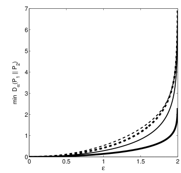
Figure 1: A plot of the minimum of the Rényi divergence $D_{\alpha}(P_{1}\|P_{2})$ subject to the constraint $|P_{1}-P_{2}|\geq\varepsilon$ where $\varepsilon\in[0,2)$. The curves in this plot correspond to $\alpha=0.25$ (thick solid curve), $\alpha=0.50$ (thin solid curve), $\alpha=0.75$ (thick dashed curve), and $\alpha=1.00$ (thin dashed curve, referring to the relative entropy).

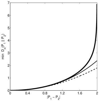
Figure 2: A plot of the minimum of the Rényi divergence $D_{\alpha}(P_{1}\|P_{2})$ of order $\alpha=0.90$ subject to the constraint $|P_{1}-P_{2}|\geq\varepsilon\in[0,2)$. The exact minimum (thick solid curve) is compared with the Pinsker-type lower bound in [14, Corollary 9] (the thin solid curve), and its weaker version in [14, Corollary 6] (the dashed curve).

III The Locus of $(D(Q\|P_{1}),D(Q\|P_{2}))$ With a Constrained Total Variation Distance

In this section, we address the following question:

Question 1

What is the locus of the points $\bigl{(}D(Q\|P_{1}),D(Q\|P_{2})\bigr{)}$ if $P_{1},P_{2},Q$ are arbitrary probability measures which are mutually absolutely continuous, and $|P_{1}-P_{2}|\geq\varepsilon$ for a given value $\varepsilon\in(0,2)$ ? (none of the three probability measures is fixed).

The present section provides an exact characterization of this locus in view of the solution to the minimization problem in Section II, and the following lemma:

Lemma 4

Let $P_{1},P_{2},Q$ be pairwise mutually absolutely continuous probability measures defined on a measurable space $(\mathcal{A},\mathscr{F})$. Then, for $\alpha\in(0,1)\cup(1,\infty)$,

$$D_{\alpha}(P_{1}\|P_{2})=D(Q\|P_{2})+\tfrac{\alpha}{1-\alpha}\cdot D(Q\|P_{1})+\tfrac{1}{\alpha-1}\cdot D(Q\|Q_{\alpha})$$ (25)

where the probability measure $Q_{\alpha}$ is given by

$$\frac{\mathrm{d}Q_{\alpha}}{\mathrm{d}Q}\,(x)=\frac{\left(\frac{\mathrm{d}P_{1}}{\mathrm{d}Q}\,(x)\right)^{\alpha}\left(\frac{\mathrm{d}P_{2}}{\mathrm{d}Q}\,(x)\right)^{1-\alpha}}{\displaystyle{\int}_{\mathcal{A}}{\left(\frac{\mathrm{d}P_{1}}{\mathrm{d}Q}\,(u)\right)^{\alpha}}\,\left(\frac{\mathrm{d}P_{2}}{\mathrm{d}Q}\,(u)\right)^{1-\alpha}\,\mathrm{d}Q(u)},\quad\forall\,x\in\mathcal{A}.$$ (26)

Proof:

See Appendix E. ∎

As a corollary of Lemma 4, the following tight inequality holds, which is attributed to van Erven [7, Lemma 6.6] and Shayevitz [39, Section IV.B.8]). It will be useful for the continuation of this section, jointly with the results of Section II.

Corollary 2

Let $P_{1}\ll\gg P_{2}$ be mutually absolutely continuous discrete probability measures defined on a common set $\mathcal{A}$. If $\alpha\in(0,1)$ then

$$\tfrac{\alpha}{1-\alpha}\cdot D(Q\|P_{1})+D(Q\|P_{2})\geq D_{\alpha}(P_{1}\|P_{2})$$ (27)

with equality if and only if, for every $x\in\mathcal{A}$,

$$Q(x)=\frac{P_{1}(x)^{\alpha}\,P_{2}(x)^{1-\alpha}}{\sum_{u\in\mathcal{A}}P_{1}(u)^{\alpha}\,P_{2}(u)^{1-\alpha}}.$$ (28)

For $\alpha>1$, inequality (27) is reversed with the same necessary and sufficient condition for an equality.

Remark 3

The knowledge of the maximizing probability measure in (28) is required for the characterization of the exact locus which is studied in this section.

The exact locus of the points $\bigl{(}D(Q\|P_{1}),D(Q\|P_{2})\bigr{)}$ is determined as follows: let $|P_{1}-P_{2}|\geq\varepsilon$ for a fixed $\varepsilon\in(0,2)$, and let $\alpha\in(0,1)$ be chosen arbitrarily. By the tight lower bound in Section II, we have

$$D_{\alpha}(P_{1}\|P_{2})\geq g_{\alpha}(\varepsilon)$$ (29)

where $g_{\alpha}$ is expressed in (13). For $\alpha\in(0,1)$ and for a fixed value of $\varepsilon\in(0,2)$, let $p=p^{\star}$ and $q=q^{\star}$ in $(0,1)$ be set to achieve the global minimum in (13) (note that, without loss of generality, one can assume that $p\geq q$ since if $(p,q)$ achieves the minimum in (13) then also $(1-p,1-q)$ achieves the same minimum). Consequently, the lower bound in (29) is attained by probability measures $P_{1},P_{2}$ which are defined on a binary alphabet (see Lemma 2) with

$$\begin{split}&P_{1}(0)=p^{\star}=p^{\star}(\alpha,\varepsilon),\quad P_{1}(1)=1-p^{\star};\\ &P_{2}(0)=q^{\star}=q^{\star}(\alpha,\varepsilon),\quad P_{2}(1)=1-q^{\star}.\end{split}$$ (30)

From Corollary 2 and (29), (30), it follows that for every $\alpha\in(0,1)$

$$g_{\alpha}(\varepsilon)\leq D(Q\|P_{2})+\tfrac{\alpha}{1-\alpha}\cdot D(Q\|P_{1})$$ (31)

where equality in (31) holds if $P_{1}$ and $P_{2}$ are the probability measures in (30) which are defined on a binary alphabet, and $Q$ is the respective probability measure in (28) which is therefore also defined on a binary alphabet. Hence, there exists a triple of probability measures $P_{1},P_{2},Q$ which are defined on a binary alphabet and satisfy (31) with equality, and these probability measures are easy to calculate for every $\alpha\in(0,1)$ and $\varepsilon\in(0,2)$.

Remark 4

Similarly to (31), since $|P_{1}-P_{2}|=|P_{2}-P_{1}|$, it follows from (31) that

$$g_{\alpha}(\varepsilon)\leq D(Q\|P_{1})+\tfrac{\alpha}{1-\alpha}\cdot D(Q\|P_{2}).$$ (32)

By multiplying both sides of (32) by $\tfrac{1-\alpha}{\alpha}$ and relying on the skew-symmetry property in (19), it follows that (32) is equivalent to

$$g_{1-\alpha}(\varepsilon)\leq D(Q\|P_{2})+\tfrac{1-\alpha}{\alpha}\cdot D(Q\|P_{1})$$

which is (31) when $\alpha\in(0,1)$ is replaced by $1-\alpha$. Hence, since (31) holds for every $\alpha\in(0,1)$, there is no additional information in (32).

Theorem 1

The exact locus of $\bigl{(}D(Q\|P_{1}),D(Q\|P_{2})\bigr{)}$ in the setting of Question 1 is the convex region whose boundary is the convex envelope of all the straight lines

$$D(Q\|P_{2})+\tfrac{\alpha}{1-\alpha}\cdot D(Q\|P_{1})=g_{\alpha}(\varepsilon),\quad\forall\,\alpha\in(0,1)$$ (33)

(i.e., the boundary is the pointwise maximum of the set of straight lines in (33) for $\alpha\in(0,1)$). Furthermore, all the points in this convex region, including its boundary, are attained by probability measures $P_{1},P_{2},Q$ which are defined on a binary alphabet.

Proof:

Let $P_{1},P_{2},Q$ be arbitrary probability measures which are mutually absolutely continuous and satisfy the $\varepsilon$ separation condition for $P_{1}$ and $P_{2}$ in total variation. In view of Corollary 2 and since by definition $D_{\alpha}(P_{1}\|P_{2})\geq g_{\alpha}(\varepsilon)$, it follows that the point $\bigl{(}D(Q\|P_{1}),D(Q\|P_{2})\bigr{)}$ satisfies

$$D(Q\|P_{2})+\tfrac{\alpha}{1-\alpha}\cdot D(Q\|P_{1})\geq g_{\alpha}(\varepsilon)$$ (34)

for every $\alpha\in(0,1)$; this implies that every such a point is either on or above the convex envelope of the parameterized straight lines in (33).

We next prove that a point which is below the convex envelope of the lines in (33) cannot be achieved under the constraint $|P_{1}-P_{2}|\geq\varepsilon$. The reason for this claim is because for such a point $\bigl{(}D(Q\|P_{1}),D(Q\|P_{2})\bigr{)}$, there is some $\alpha\in(0,1)$ for which

$$D(Q\|P_{2})+\tfrac{\alpha}{1-\alpha}\cdot D(Q\|P_{1})<g_{\alpha}(\varepsilon)$$ (35)

Since under the $\varepsilon$ separation condition for $P_{1}$ and $P_{2}$ in total variation distance, $D_{\alpha}(P_{1}\|P_{2})\geq g_{\alpha}(\varepsilon)$, then for such $\alpha\in(0,1)$, inequality (27) is violated; in view of Corollary 2, this yields that the point is not achievable under the constraint $|P_{1}-P_{2}|\geq\varepsilon$. As an interim conclusion, it follows that the exact locus of the achievable points is the set of all points in the plane $\bigl{(}D(Q\|P_{1}),D(Q\|P_{2})\bigr{)}$ which are on or above the convex envelope of the parameterized straight lines in (33) for $\alpha\in(0,1)$.

The next step aims to show that an arbitrary point which is located at the boundary of this region can be obtained by a triplet of probability measures $(P_{1}^{\star},P_{2}^{\star},Q^{\star})$ which are defined on a binary alphabet, and satisfy $|P_{1}^{\star}-P_{2}^{\star}|=\varepsilon$. To that end, note that every point which is on the boundary of this region is a tangent point to one of the straight lines in (33) for some $\alpha\in(0,1)$. Accordingly, the proper probability measures $P_{1}^{\star}$, $P_{2}^{\star}$ and $Q^{*}$ can be determined as follows for a given $\varepsilon\in(0,2)$:

1. Find the slope $s<0$ of the tangent line at the selected point on the boundary; in view of (33), $s=-\tfrac{\alpha}{1-\alpha}$ yields $\alpha=-\frac{s}{1-s}\in(0,1)$.

2. In view of Proposition 3, determine $p_{1}^{\star},p_{2}^{\star}\in(0,1)$ such that $|p_{1}^{\star}-p_{2}^{\star}|=\tfrac{\varepsilon}{2}$ and $d_{\alpha}(p_{1}^{\star}\|p_{2}^{\star})=g_{\alpha}(\varepsilon)$. Consequently, let $P_{1}^{\star}$ and $P_{2}^{\star}$ be the probability measures which are defined on the binary alphabet with $P_{1}^{\star}(0)=p_{1}^{\star}$ and $P_{2}^{\star}(0)=p_{2}^{\star}$.

3. The respective probability measure $Q^{\star}=Q^{\star}_{\alpha}$ is calculated from (28), and it is therefore also defined on the binary alphabet.

Finally, we show that every interior point in the achievable region can be attained as well by a proper selection of $P_{1}^{\star}$, $P_{2}^{\star}$ and $Q^{\star}$ which are defined on a binary alphabet. To that end, note that every such interior point is located at the boundary of the locus of $\bigl{(}D(Q\|P_{1}),D(Q\|P_{2})\bigr{)}$ under the constraint $|P_{1}-P_{2}|\geq\mkern 1.5mu\overline{\mkern-1.5mu\varepsilon\mkern-1.5mu}\mkern 1.5mu$ with some $\mkern 1.5mu\overline{\mkern-1.5mu\varepsilon\mkern-1.5mu}\mkern 1.5mu\in(\varepsilon,2)$; this follows from the fact that $g_{\alpha}(\cdot)$ is a strictly monotonically increasing and continuous function in $(0,2)$, which tends to infinity as we let $\varepsilon$ tend to 2 (see Lemma 10). It therefore follows that the suitable triplet of probability measures $(P_{1}^{\star},P_{2}^{\star},Q^{\star})$ can be obtained by the same algorithm used for points on the boundary of this region, except for replacing $\varepsilon$ by the larger value $\mkern 1.5mu\overline{\mkern-1.5mu\varepsilon\mkern-1.5mu}\mkern 1.5mu$.

This concludes the proof by first characterizing the exact locus of points, and then demonstrating that every point in this convex region (including its boundary) is attained by probability measures which are defined on the binary alphabet; the proof is also constructive in the sense of providing an algorithm to calculate such probability measures $P_{1}^{\star},P_{2}^{\star},Q^{\star}$ for an arbitrary point in this closed and convex region. ∎

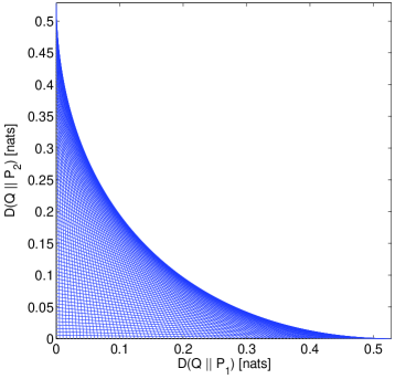
Figure 3: The exact locus of $(D(Q\|P_{1}),D(Q\|P_{2}))$ where $P_{1},P_{2}$ are arbitrary probability measures with $|P_{1}-P_{2}|\geq 1$ with $\varepsilon=1$. The exact locus of these relative entropies includes all the points on and above the convex envelope of the straight lines in (33), which is the convex and closed region painted in white.

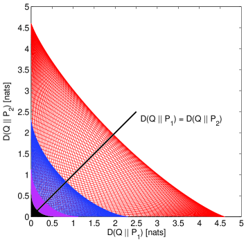
Figure 4: This plot shows the 4 exact loci of $(D(Q\|P_{1}),D(Q\|P_{2}))$ where $P_{1},P_{2}$ are arbitrary probability measures such that $|P_{1}-P_{2}|\geq\varepsilon$, with $\varepsilon=1.00,1.40,1.80,1.98$, and $Q\ll P_{1},P_{2}$ is an arbitrary probability measure. The exact locus which is above the convex envelope for the respective value of $\varepsilon$ (painted in white) shrinks as the value of $\varepsilon$ is increased, especially when $\varepsilon$ is close (from below) to 2. The intersection of the boundary of the exact locus, for a given $\varepsilon\in[0,2)$, with the straight line $D(Q\|P_{1})=D(Q\|P_{2})$ (passing through the origin) is at the point $\bigl{(}-\tfrac{1}{2}\,\log(1-\varepsilon^{2}),\,-\tfrac{1}{2}\,\log(1-\varepsilon^{2})\bigr{)}$; the equal coordinates of this point are the minimum of the Chernoff information subject to a given total variation distance $\varepsilon$.

As it is shown in Figure 4, the boundaries of these regions become less curvy as $\varepsilon\uparrow 2$.

A Geometric Interpretation of the Minimal Chernoff Information with a Constraint on the Variational Distance

Consider the point in Figure 4 which, in the plane of $\bigl{(}D(Q\|P_{1}),D(Q\|P_{2})\bigr{)}$, is the intersection of the straight line $D(Q\|P_{1})=D(Q\|P_{2})$ and the boundary of the convex region which is characterized in Theorem 1 for an arbitrary $\varepsilon\in(0,2)$.

In view of the proof of Theorem 1, this intersection point satisfies $D(Q_{\alpha}\|P_{1})=D(Q_{\alpha}\|P_{2})$ for some $\alpha\in(0,1)$, for $P_{1},P_{2}$ which are probability measures defined on a binary alphabet with $|P_{1}-P_{2}|=\varepsilon$, and $Q_{\alpha}$ is given in (28). The equal coordinates of this intersection point are therefore equal to the Chernoff information $C(P_{1},P_{2})$ (see [5, Section 11.9]). Due to the symmetry of this region with respect to the straight line $D(Q\|P_{1})=D(Q\|P_{2})$ (this follows from the symmetry property $|P_{1}-P_{2}|=|P_{2}-P_{1}|$), the slope of the tangent line to the boundary of the convex region at this intersection point is $s=-1$ (see Figure 4). This yields that $\alpha=-\frac{s}{1-s}=\tfrac{1}{2}$, and from Proposition 2, $g_{\alpha}(\varepsilon)=-\log\bigl{(}1-\frac{1}{4}\,\varepsilon^{2}\bigr{)}$. Hence, from (33) with $\alpha=\tfrac{1}{2}$, the equal coordinates of this intersection point are given by

$$D(Q\|P_{1})=D(Q\|P_{2})=-\tfrac{1}{2}\,\log\bigl{(}1-\frac{1}{4}\,\varepsilon^{2}\bigr{)}.$$ (36)

Based on [31, Proposition 2], this value is equal to the minimum of the Chernoff information subject to an $\varepsilon$ separation constraints for $P_{1}$ and $P_{2}$ in total variation distance. We next calculate the probability measures $P_{1}^{\star}$, $P_{2}^{\star}$ and $Q^{\star}$ which attain this intersection point. Eq. (13) with $\alpha=\frac{1}{2}$ yields

$$-2\log\bigl{(}\sqrt{pq}+\sqrt{(1-p)(1-q)}\bigr{)}=-\log\bigl{(}1-\tfrac{1}{4}\varepsilon^{2}\bigr{)}$$ (37)

such that $p,q\in[0,1]$ and $|p-q|=\frac{\varepsilon}{2}$. A possible solution of this equation is $p=\frac{2+\varepsilon}{4}$ and $q=\frac{2-\varepsilon}{4}$, so the respective probability measures $P_{1}^{\star},P_{2}^{\star}$ which are defined on the binary alphabet satisfy $P_{1}^{\star}(0)=\frac{2+\varepsilon}{4}$ and $P_{2}^{\star}(0)=\frac{2-\varepsilon}{4}$; consequently, from (28), $Q(0)=Q(1)=\tfrac{1}{2}$ is the equiprobable distribution on the binary alphabet.

As a byproduct of the characterization of the convex region in Theorem 1, it follows that the straight line $D(Q\|P_{1})=D(Q\|P_{2})$ (in the plane of Figure 4) intersects the boundary of the convex region which is specified in Theorem 1 at the point whose coordinates are equal to the minimized Chernoff information subject to the constraint $|P_{1}-P_{2}|\geq\varepsilon$. The equal coordinates of each of the 4 intersection points in Figure 4, which refer to $\varepsilon=1.00,1.40,1.80,1.98$, are equal to $-\tfrac{1}{2}\,\log\bigl{(}1-\frac{1}{4}\,\varepsilon^{2}\bigr{)}=0.144,0.337,0.830,1.959$ nats, respectively.

IV A Performance Bound for Coded Communications via the Rényi Divergence

IV-A New Exponential Upper Bound

This section derives an exponential upper bound on the performance of binary linear block codes, expressed in terms of the Rényi divergence. Similarly to [19], [20], [21], [23], [25], [33, Section 3.B], [36], [40] and [43], the upper bound in the next theorem quantifies the degradation in the performance of block codes under ML decoding in terms of the deviation of their distance spectra from the binomially distributed (average) distance spectrum of the capacity-achieving ensemble of random block codes.

Theorem 2

Consider a binary linear block code of length $N$ and rate $R=\frac{\log(M)}{N}$ where $M$ designates the number of codewords. Let $S_{0}=0$ and, for $l\in\{1,\ldots,N\}$, let $S_{l}$ be the number of non-zero codewords of Hamming weight $l$. Assume that the transmission of the code takes place over a memoryless, binary-input and output-symmetric channel. Then, the block error probability under ML decoding satisfies

$$P_{\text{e}}=P_{\text{e}|0}<\exp\left(-N\,\sup_{r\geq 1}\,\max_{0\leq\rho^{\prime}\leq\frac{1}{r}}\,\left[E_{0}\left(\rho^{\prime},\underline{q}=\bigl{(}\tfrac{1}{2},\tfrac{1}{2}\bigr{)}\right)-\rho^{\prime}\left(rR+\frac{D_{s}(P_{N}\|Q_{N})}{N}\right)\right]\right)$$ (38)

where $s\triangleq s(r)=\frac{r}{r-1}$ for $r\geq 1$ (with the convention that $s=\infty$ for $r=1$), $Q_{N}$ is the binomial distribution with parameter $\tfrac{1}{2}$ and $N$ independent trials (i.e., $Q_{N}(l)=2^{-N}{N\choose l}$ for $l\in\{0,1,\ldots,N\}$), $P_{N}$ is the PMF defined by $P_{N}(l)=\frac{S_{l}}{M-1}$ for $l\in\{0,\ldots,N\}$, $D_{s}(\cdot\|\cdot)$ is the Rényi divergence of order $s$ (i.e., $D_{s}(P\|Q)=\frac{1}{s-1}\,\log\left(\sum_{x}P(x)^{s}Q(x)^{1-s}\right)$ where $s>1$ here), and $E_{0}(\rho,\underline{q})$ designates the Gallager random coding error exponent in [12, Eq. (5.6.14)].

Before proving Theorem 2, we relate this exponential bound to previously reported bounds.

Remark 5

Note that the loosening of the bound by taking $r=1$ and, respectively, $s=\infty$ gives the upper bound

$$P_{\text{e}}=P_{\text{e}|0} <\exp\left(-N\,\max_{0\leq\rho^{\prime}\leq 1}\left[E_{0}\left(\rho^{\prime},\underline{q}=\bigl{(}\tfrac{1}{2},\tfrac{1}{2}\bigr{)}\right)-\rho^{\prime}\left(R+\frac{D_{\infty}(P_{N}\|Q_{N})}{N}\right)\right]\right)$$

$$\stackrel{{\scriptstyle(\text{a})}}{{=}}\exp\left(-N\,E_{\text{r}}\left(R+\frac{D_{\infty}(P_{N}\|Q_{N})}{N}\right)\right)$$

$$\stackrel{{\scriptstyle(\text{b})}}{{=}}\exp\left(-N\,E_{\text{r}}\left(R+\frac{1}{N}\,\log\max_{0\leq l\leq N}\frac{P_{N}(l)}{Q_{N}(l)}\right)\right)$$

$$\stackrel{{\scriptstyle(\text{c})}}{{=}}\exp\left(-N\,E_{\text{r}}\left(R+\frac{1}{N}\,\log\max_{0\leq l\leq N}\frac{S_{l}}{e^{-N(\log 2-R)}{N\choose{l}}}\right)\right)$$

which coincides with the Shulman-Feder bound [40]. Equality (a) follows from the definition of the Gallager random coding exponent $E_{\text{r}}(R)$ in [12, Eq. (5.6.16)] where the symmetric input distribution $\underline{q}=\bigl{(}\tfrac{1}{2},\tfrac{1}{2}\bigr{)}$ is the optimal input distribution for any memoryless, binary-input output-symmetric channel, equality (b) follows from the expression of the Rényi divergence of order infinity (see, e.g., [8, Theorem 6]), and equality (c) follows from the definition of the PMFs $P_{N}$ and $Q_{N}$ in Theorem 2.

Remark 6

The proof of Theorem 2 is based on the framework of the Gallager bounds in [32, Chapter 4] and [36]. Specifically, it has an overlap with [36, Appendix A]. Unlike the analysis in [36, Appendix A], working with the Rényi divergence of order $s\geq 1$, instead of the relative entropy as a lower bound (see [36, Eq. (A19)]) reveals a need for an optimization of the error exponent, which leads to the error exponent in Theorem 2. Namely, if the value of $r\geq 1$ is increased then the value of $s=\frac{r}{r-1}\geq 1$ is decreased, and therefore $D_{s}(P_{N}\|Q_{N})$ is also decreased (unless it is zero, see [8, Theorem 3]; note that $P_{N}$ and $Q_{N}$ do not depend on the parameters $r$ and $s$, so they stay un-affected by varying the values of these parameters). The maximization of the error exponent in Theorem 2 aims at finding a proper balance between the two summands $rR$ and $\frac{D_{s}(P_{N}\|Q_{N})}{N}$ on the right-hand side of (38), while also performing an optimization over the second dependent variable $\rho^{\prime}\in\bigl{[}0,\frac{1}{r}\bigr{]}$.

We proceed now with the proof of Theorem 2.

Proof:

The proof of Theorem 2 is based on the framework of the Gallager bounds in [32, Chapter 4] and [36]. Specifically, it relies on [36, Appendix A]. We explain in the following how our proof differs from the analysis in [36, Appendix A]. From [36, Eq. (A17)], we have that for every $\rho^{\prime}\in\bigl{[}0,\frac{1}{r}\bigr{]}$

$$P_{\text{e}|0} <M^{\rho^{\prime}r}\,\exp\left(-N\,E_{0}\Bigl{(}\rho^{\prime},\underline{q}=\Bigl{(}\frac{1}{2},\frac{1}{2}\Bigr{)}\Bigr{)}\right)\,\left(\sum_{l=0}^{N}\,Q_{N}(l)\,\left(\frac{P_{N}(l)}{Q_{N}(l)}\right)^{s}\right)^{\frac{r\rho^{\prime}}{s}}.$$ (39)

From this point, we deviate from the analysis in [36, Appendix A]. Since $\frac{1}{r}+\frac{1}{s}=1$ where $r,s\geq 1$, we have

$$\left(\sum_{l=0}^{N}\,Q_{N}(l)\,\left(\frac{P_{N}(l)}{Q_{N}(l)}\right)^{s}\right)^{\frac{r\rho^{\prime}}{s}}$$

$$=\exp\left(\frac{r\rho^{\prime}}{s}\cdot\log\left(\sum_{l=0}^{N}\,P_{N}(l)^{s}\,Q_{N}(l)^{1-s}\right)\right)$$

$$=\exp\left(\frac{\rho^{\prime}}{s-1}\cdot\log\left(\sum_{l=0}^{N}\,P_{N}(l)^{s}\,Q_{N}(l)^{1-s}\right)\right)$$

$$=\exp\bigl{(}\rho^{\prime}D_{s}(P_{N}\|Q_{N})\bigr{)}$$ (40)

where $D_{s}(P_{N}\|Q_{N})$ is the Rényi divergence of order $s$ from $P_{N}$ to $Q_{N}$. This enables to refer to the Rényi divergence of order $s\geq 1$, instead of lower bounding this quantity by the relative entropy, and consequently loosening the bound (see [36, Eq. (A19)]). Note that since the Rényi divergence is monotonically increasing in its order (see, e.g., [8, Theorem 3]) and the Rényi divergence of order 1 is particularized to the relative entropy, the inequality $D_{s}(P_{N}\|Q_{N})\geq D(P_{N}\|Q_{N})$ holds. The combination of (39) and (40) gives

$$P_{\text{e}|0} <\exp(NR\rho^{\prime}r)\,\exp\left(-N\,E_{0}\Bigl{(}\rho^{\prime},\underline{q}=\bigl{(}\tfrac{1}{2},\tfrac{1}{2}\bigr{)}\Bigr{)}\right)\,\exp\bigl{(}\rho^{\prime}D_{s}(P_{N}\|Q_{N})\bigr{)}$$

$$=\exp\left(-N\left[E_{0}\Bigl{(}\rho^{\prime},\underline{q}=\bigl{(}\tfrac{1}{2},\tfrac{1}{2}\bigr{)}\Bigr{)}-\rho^{\prime}\biggl{(}rR+\frac{D_{s}(P_{N}\|Q_{N})}{N}\biggr{)}\right]\right),\quad 0\leq\rho^{\prime}\leq\frac{1}{r}.$$ (41)

A maximization of the error exponent in (41) with respect to the parameters $r\geq 1$ and $\rho^{\prime}\in[0,\frac{1}{r}]$ (recall that $s=s(r)=\frac{r}{r-1}>1$) gives the upper bound in (38). ∎

IV-B Application of Theorem 2

An efficient use of Theorem 2 for the performance evaluation of binary linear block codes (or coee ensembles) is suggested in the following by borrowing a concept of bounding from [23], which has been further studied, e.g., in [32], [33], [43], and combining it with the new bound in Theorem 2. In order to utilize the Shulman-Feder bound for binary linear block codes in a clever way, it has been suggested in [23] to partition the binary linear block code $\mathcal{C}$ into two subcodes $\mathcal{C}_{1}$ and $\mathcal{C}_{2}$ where $\mathcal{C}_{1}\cup\mathcal{C}_{2}=\mathcal{C}$ and $\mathcal{C}_{1}\cap\mathcal{C}_{2}=\{0\}$ is the all-zero codeword. The first subcode $\mathcal{C}_{1}$ contains the all-zero codeword and all the codewords of $\mathcal{C}$ whose Hamming weights $l$ belong to a subset $\mathcal{L}\subseteq\{1,2,...,N\}$, while $\mathcal{C}_{2}$ contains the other codewords of $\mathcal{C}$ which have Hamming weights of $l\in\mathcal{L}^{\mathrm{c}}\triangleq\{1,2,...,N\}\setminus\mathcal{L}$, together with the all-zero codeword. From the symmetry of the channel, $P_{\text{e}}=P_{\text{e}|0}\leq P_{\text{e}|0}(\mathcal{C}_{1})+P_{\text{e}|0}(\mathcal{C}_{2})$ where $P_{\text{e}|0}(\mathcal{C}_{1})$ and $P_{\text{e}|0}(\mathcal{C}_{2})$ designate the conditional ML decoding error probabilities of $\mathcal{C}_{1}$ and $\mathcal{C}_{2}$, respectively, given that the all-zero codeword is transmitted. Note that although the code $\mathcal{C}$ is linear, its two subcodes $\mathcal{C}_{1}$ and $\mathcal{C}_{2}$ are in general non-linear. One can rely on different upper bounds on the conditional error probabilities $P_{\text{e}|0}(\mathcal{C}_{1})$ and $P_{\text{e}|0}(\mathcal{C}_{2})$, i.e., we may bound $P_{\text{e}|0}(\mathcal{C}_{1})$ by invoking Theorem 2, due to its tightening of the Shulman-Feder bound (see Remark 5), and also rely on an alternative approach for obtaining an upper bound on $P_{\text{e}|0}(\mathcal{C}_{2})$ (e.g., it is possible to rely on the union bound with respect to the fixed composition codes of the subcode $\mathcal{C}_{2}$). The idea behind this partitioning is to include in the subcode $\mathcal{C}_{1}$ the codewords of all the Hamming weights whose distance spectrum is close enough to the binomial distribution $Q_{N}$ (see Theorem 2) in the sense that the additional term $\frac{D_{s}(P_{N}\|Q_{N})}{N}$ in the exponent of (38) has a marginal effect on the conditional ML decoding error probability of the subcode $\mathcal{C}_{1}$.

Theorem 2 can be applied as well to ensembles of binary linear block codes. The verify this claim, let $\mathcal{C}$ be an ensemble of binary linear block codes. The proof of Theorem 2 follows from the Duman and Salehi bounding technique [36] which leads to the derivation of [36, Eq. (A.11)]. By taking the expectation on the RHS of [36, Eq. (A.11)] with respect to the code ensemble $\mathcal{C}$ and invoking Jensen’s inequality, the same bound holds while $S_{l}$, as it is defined in Theorem 2, is replaced by the expectation $\overline{S_{l}}\triangleq\mathbb{E}_{\mathcal{C}}\bigl{[}S_{l}\bigr{]}$ with respect to the code ensemble $\mathcal{C}$. This enables to replace $P_{N}$ on the RHS of (38) with $\overline{P}_{N}$ where

$$\overline{P}_{N}(l)\triangleq\frac{\mathbb{E}_{\mathcal{C}}\bigl{[}S_{l}\bigr{]}}{M-1},\quad\forall\,l\in\{0,\ldots,N\},$$

which therefore justifies the generalization of Theorem 2 to code ensembles of binary linear block codes.

As it is exemplified in Section IV-C, Theorem 2 can be efficiently applied to ensembles of turbo-like codes in the same way that it was demonstrated to be efficient in [43]. Similarly to Theorem 2, the bound in [43, Theorem 3.1] forms another refinement of the Shulman-Feder bound, and the novelty in the former bound is the obtained tightening of the Shulman-Feder bound via the use of the Rényi divergence.

IV-C An Example: Performance Bounds for an Ensemble of Turbo-Block Codes

We conclude this section by an example which applies this bounding technique to the ensemble of uniformly interleaved turbo codes whose two component codes are chosen uniformly at random from the ensemble of (1072, 1000) binary systematic linear block codes. The transmission of these codes takes place over an additive white Gaussian noise (AWGN) channel, and the codes are BPSK modulated and coherently detected. The calculation of the average distance spectrum of this ensemble has been performed in [43, Section 5.D], which is required for the calculation of the upper bound in (38) where the PD $P_{N}$ is replaced by its expected value over the ensemble (i.e., the normalization of the average distance spectrum by the number of codewords, as it is defined in Theorem 2). In the following, two upper bounds on the block error probability are compared under ML decoding: the first one is the tangential-sphere bound (TSB) of Herzberg and Poltyrev (see [18], [26], [32, Section 3.2.1]), and the second bound follows from the suggested combination of the union bound and Theorem 2. Note that an optimal partitioning has been performed, in a way which is conceptually similar to [43, Algorithm 1], for obtaining the tightest bound which is obtained by combining the union bound and Theorem 2.

A comparison of the two bounds shows an advantage of the latter combined bound over the TSB in a similar way to [43, upper plot of Fig. 8] (e.g., providing a gain of about 0.2 dB over the TSB for a block error probability of $10^{-3}$). Note that the Shulman-Feder bound is rather loose in this case due to the significant deviation of the ensemble distance spectrum from the binomial distribution at low and high Hamming weights. Furthermore, we note that the advantage of the proposed bound over the TSB in this example is consistent with the analysis in [26] and [42], demonstrating a gap between the random coding error exponent of Gallager and the corresponding error exponents that follow from the TSB and some of its improved versions. Recall that the random coding error exponent of Gallager achieves the channel capacity, whereas the random coding error exponent that follows from the TSB (or some of its improved variants) does not achieve the capacity of a binary-input AWGN channel for BPSK modulated fully random block codes, where the gap to capacity is especially pronounced for high coding rates. In this example, the rate of the ensemble is 0.8741 bits per channel use.

Appendix A Proofs of Lemmas 10 and 2

A-A Proof of Lemma 10

For $\alpha=\tfrac{1}{2}$, $D_{\frac{1}{2}}(P\|Q)=-2\log Z(P,Q)$ where $Z(P,Q)\triangleq\sum_{x}\sqrt{P(x)Q(x)}$ denotes the Bhattacharyya coefficient between the two PDs $P,Q$. We have

$$D_{\frac{1}{2}}(P\|Q)\geq-\log\left(1-\tfrac{1}{4}\,\varepsilon^{2}\right)$$ (I.1)

where $|P-Q|=\varepsilon$ (see, e.g., [31, Proposition 1]; inequality (I.1) is known in quantum information theory with respect to the relation between the trace distance and fidelity [47, Section 9.3]). Hence, (I.1) implies that (10) holds for $\alpha=\tfrac{1}{2}$. Since $D_{\alpha}(P\|Q)$ is monotonically increasing in its order $\alpha$ (see [8, Theorem 3]), it follows that (10) also holds for $\alpha\geq\tfrac{1}{2}$. Finally, due to the skew-symmetry property of $D_{\alpha}$ (see [8, Proposition 2]) where $D_{\alpha}(P\|Q)=\left(\tfrac{\alpha}{1-\alpha}\right)D_{1-\alpha}(Q\|P)$ for $\alpha\in(0,1)$, and since the total variation distance is a symmetric measure and $\tfrac{\alpha}{1-\alpha}>0$ for $\alpha\in(0,1)$, the satisfiability of (10) for $\alpha\in(\tfrac{1}{2},1)$ yields that it also holds for $\alpha\in(0,\tfrac{1}{2})$.

A-B Proof of Lemma 2

Let $P_{1}\ll P_{2}$ be probability measures which are defined on a common measurable space $(\mathcal{A},\mathscr{F})$. Denote by $\phi\colon\mathcal{A}\rightarrow\{1,2\}$ the mapping given by

$$\phi(x)=\left\{\begin{array}[]{ll}1,&\quad\mbox{if $\frac{\mathrm{d}P_{1}}{\mathrm{d}P_{2}}(x)\geq 1$,}\\ 2,&\quad\mbox{if $\frac{\mathrm{d}P_{1}}{\mathrm{d}P_{2}}(x)<1$}\end{array}\right.$$

and let $Q_{i}$, for $i\in\{1,2\}$, be given by

$$Q_{i}(j)\triangleq\int_{\{x\in\mathcal{A}\colon\phi(x)=j\}}\mathrm{d}P_{i}(x),\quad\forall\,i,j\in\{1,2\}.$$ (I.2)

Consequently, we have

$$|P_{1}-P_{2}| =\int_{\mathcal{A}}\left|\frac{\mathrm{d}P_{1}}{\mathrm{d}P_{2}}(x)-1\right|\,\mathrm{d}P_{2}(x)$$

$$=\int_{\{x\in\mathcal{A}\colon\phi(x)=1\}}\left(\frac{\mathrm{d}P_{1}}{\mathrm{d}P_{2}}(x)-1\right)\,\mathrm{d}P_{2}(x)+\int_{\{x\in\mathcal{A}\colon\phi(x)=2\}}\left(1-\frac{\mathrm{d}P_{1}}{\mathrm{d}P_{2}}(x)\right)\,\mathrm{d}P_{2}(x)$$

$$=\bigl{(}Q_{1}(1)-Q_{2}(1)\bigr{)}+\bigl{(}Q_{2}(2)-Q_{1}(2)\bigr{)}$$

$$=\sum_{j\in\{1,2\}}\bigl{|}Q_{1}(j)-Q_{2}(j)\bigr{|}$$

$$=|Q_{1}-Q_{2}|.$$ (I.3)

From the data processing theorem for the Rényi divergence (see [8, Theorem 9]),

$$D_{\alpha}(P_{1}\|P_{2})\geq D_{\alpha}(Q_{1}\|Q_{2})$$ (I.4)

where $Q_{1}$ and $Q_{2}$ are the probability measures which are defined on the binary alphabet (see (I.2)). The lemma follows by combining (A-B) and (I.4).

Appendix B Proof of Proposition 2

Eq. (15) follows from the equality $D_{\frac{1}{2}}(P\|Q)=-2\log Z(P,Q)$ where $Z(P,Q)$ is the Bhattacharyya coefficient between $P,Q$, and since (see [31, Proposition 1])

$$\max_{P,Q\colon|P-Q|=\varepsilon}Z(P,Q)=\sqrt{1-\tfrac{1}{4}\,\varepsilon^{2}},\quad\forall\,\varepsilon\in[0,2).$$

To prove (18), note that $D_{2}(P_{1}\|P_{2})=\log\bigl{(}1+\chi^{2}(P_{1},P_{2})\bigr{)}$ where

$$\chi^{2}(P_{1}\|P_{2})\triangleq\int\left(\frac{\mathrm{d}P_{1}}{\mathrm{d}P_{2}}-1\right)^{2}\,\mathrm{d}P_{2}$$

denotes the $\chi^{2}$-divergence between the probability measures $P_{1}$ and $P_{2}$ (which is the Hellinger divergence of order 2). One can derive a closed-form expression for $g_{2}$ by relying on the closed-form solution of a minimization of the $\chi^{2}$-divergence $\chi^{2}(P_{1}\|P_{2})$ subject to the constraint $|P_{1}-P_{2}|=\varepsilon\in[0,2)$, which is given by (see [29, Eq. (58)])

$$\min_{P_{1},P_{2}\colon|P_{1}-P_{2}|=\varepsilon}\chi^{2}(P_{1}\|P_{2})=\left\{\begin{array}[]{ll}\varepsilon^{2},&\quad\mbox{if $\varepsilon\in[0,1]$,}\\[2.84544pt] \frac{\varepsilon}{2-\varepsilon},&\quad\mbox{if $\varepsilon\in(1,2).$}\end{array}\right.$$

Eq. (19) follows from the skew-symmetry property of the Rényi divergence [8, Proposition 2].

The lower bound on $g_{\alpha}$ in (20) follows from (13), which implies that for $\alpha\in(0,1)$ and $\varepsilon\in[0,2)$

$$g_{\alpha}(\varepsilon)=\frac{\log\Bigl{(}\max_{p,q\in[0,1]\colon|p-q|\geq\frac{\varepsilon}{2}}\left(p^{\alpha}q^{1-\alpha}+(1-p)^{\alpha}(1-q)^{1-\alpha}\right)\Bigr{)}}{\alpha-1}$$ (II.1)

and, we have

$$0 \leq\max_{p,q\in[0,1]\colon|p-q|\geq\frac{\varepsilon}{2}}\bigl{(}p^{\alpha}q^{1-\alpha}+(1-p)^{\alpha}(1-q)^{1-\alpha}\bigr{)}$$

$$\leq\max_{p,q\in[0,1]\colon|p-q|\geq\frac{\varepsilon}{2}}p^{\alpha}q^{1-\alpha}+\max_{p,q\in[0,1]\colon|p-q|\geq\frac{\varepsilon}{2}}(1-p)^{\alpha}(1-q)^{1-\alpha}$$

$$=2\max_{p,q\in[0,1]\colon|p-q|\geq\frac{\varepsilon}{2}}p^{\alpha}q^{1-\alpha}$$

$$=2\,\max\left\{\bigl{(}1-\tfrac{1}{2}\,\varepsilon\bigr{)}^{\alpha},\,\bigl{(}1-\tfrac{1}{2}\,\varepsilon\bigr{)}^{1-\alpha}\right\}.$$ (II.2)

The lower bound on $g_{\alpha}$ in (20) follows from the combination of (II.1) and (II.2).

Appendix C Proof of Lemma 3

For $\alpha\in(0,1)$ and $\varepsilon^{\prime}\in(0,1)$, we have

$$\lim_{q\rightarrow 0^{+}}\left(1+\frac{\varepsilon^{\prime}}{q}\right)^{\alpha-1}=0,\qquad\lim_{q\rightarrow 0^{+}}\left(1+\frac{\varepsilon^{\prime}}{q}\right)^{\alpha}=+\infty,$$

$$\Longrightarrow\lim_{q\rightarrow 0^{+}}f_{\alpha,\varepsilon^{\prime}}(q)=\lim_{q\rightarrow 0^{+}}\frac{(1-\varepsilon^{\prime})^{\alpha-1}}{\left(1+\frac{\varepsilon^{\prime}}{q}\right)^{\alpha}-(1-\varepsilon^{\prime})^{\alpha}}=0,$$

and

$$\lim_{q\rightarrow(1-\varepsilon^{\prime})^{-}}\left(1-\frac{\varepsilon^{\prime}}{1-q}\right)^{\alpha-1}=+\infty,\qquad\lim_{q\rightarrow(1-\varepsilon^{\prime})^{-}}\left(1-\frac{\varepsilon^{\prime}}{1-q}\right)^{\alpha}=0,$$

$$\Longrightarrow\lim_{q\rightarrow(1-\varepsilon^{\prime})^{-}}f_{\alpha,\varepsilon^{\prime}}(q)=\lim_{q\rightarrow(1-\varepsilon^{\prime})^{-}}\frac{\left(1-\frac{\varepsilon^{\prime}}{1-q}\right)^{\alpha-1}-(1-\varepsilon^{\prime})^{1-\alpha}}{(1-\varepsilon^{\prime})^{-\alpha}-\left(1-\frac{\varepsilon^{\prime}}{1-q}\right)^{\alpha}}=+\infty.$$

This proves the two limits in (23).

We prove in the following that $f_{\alpha,\varepsilon^{\prime}}(\cdot)$ is strictly increasing on the interval $\bigl{[}\frac{1-\varepsilon^{\prime}}{2},1-\varepsilon^{\prime})$, and we also prove later in this appendix that this function is monotonically increasing on the interval $\bigl{(}0,\frac{1-\varepsilon^{\prime}}{2}\bigr{]}$. These two parts of the proof yield that $f_{\alpha,\varepsilon^{\prime}}(\cdot)$ is strictly monotonically increasing on the interval $(0,1-\varepsilon^{\prime})$. The positivity of $f_{\alpha,\varepsilon^{\prime}}$ on $(0,1-\varepsilon^{\prime})$ follows from the first limit in (23), jointly with the monotonicity of this function which is proved in the following.

For a proof that $f_{\alpha,\varepsilon^{\prime}}(\cdot)$ is strictly monotonically increasing on $\bigl{[}\frac{1-\varepsilon^{\prime}}{2},1-\varepsilon^{\prime})$, this function (see (22)) is expressed as follows:

$$f_{\alpha,\varepsilon^{\prime}}(q) =\left(1+\frac{\varepsilon^{\prime}}{q}\right)^{-1}u_{\alpha}\bigl{(}z_{\varepsilon^{\prime}}(q)\bigr{)}$$ (III.1)

where

$$z_{\varepsilon^{\prime}}(q)\triangleq\frac{1-\frac{\varepsilon^{\prime}}{1-q}}{1+\frac{\varepsilon^{\prime}}{q}}\,,$$ (III.2)

$$u_{\alpha}(t)\triangleq\left\{\begin{array}[]{ll}\frac{t^{\alpha-1}-1}{1-t^{\alpha}},&\quad\mbox{if $t\in(0,1)\cup(1,\infty)$,}\\[5.69046pt] \tfrac{1-\alpha}{\alpha},&\quad\mbox{if $t=1$.}\end{array}\right.$$ (III.5)

Note that $u_{\alpha}$ in (III.5) was defined to be continuous at $t=1$. In order to proceed, we need the following two lemmas:

Lemma III.1

Let $\varepsilon^{\prime}\in(0,1)$. The function $z_{\varepsilon^{\prime}}$ in (III.2) is strictly monotonically increasing on $\bigl{(}0,\frac{1-\varepsilon^{\prime}}{2}\bigr{]}$, and it is strictly monotonically decreasing on $\bigl{[}\frac{1-\varepsilon^{\prime}}{2},1-\varepsilon^{\prime})$. This function is also positive on $(0,1-\varepsilon^{\prime})$.

Proof:

$z_{\varepsilon^{\prime}}(q)>0$ for $q\in(0,1-\varepsilon^{\prime})$ since $1-\frac{\varepsilon^{\prime}}{1-q}>0$, and $1+\frac{\varepsilon^{\prime}}{q}>0$. In order to prove the monotonicity properties of $z_{\varepsilon^{\prime}}$, note that its derivative satisfies the equality

$$\frac{\mathrm{d}}{\mathrm{d}q}\;z_{\varepsilon^{\prime}}(q)=\varepsilon^{\prime}\,z_{\varepsilon^{\prime}}(q)\,\left(\frac{1}{q(\varepsilon^{\prime}+q)}-\frac{1}{(1-q)(1-\varepsilon^{\prime}-q)}\right)$$ (III.6)

which is derived by taking logarithms on both sides of (III.2), followed by their differentiation. By setting the derivative of $z_{\varepsilon^{\prime}}(q)$ (with respect to $q$) to zero, we have $q=\frac{1-\varepsilon^{\prime}}{2}$. Since $z_{\varepsilon^{\prime}}(q)>0$ for $q\in(0,1-\varepsilon^{\prime})$, it follows from (III.6) that $z^{\prime}_{\varepsilon^{\prime}}(q)>0$ for $q\in\bigl{(}0,\frac{1-\varepsilon^{\prime}}{2}\bigr{)}$, and $z^{\prime}_{\varepsilon^{\prime}}(q)<0$ for $q\in\bigl{(}\frac{1-\varepsilon^{\prime}}{2},1-\varepsilon^{\prime})$. Hence, $z_{\varepsilon^{\prime}}$ is strictly monotonically increasing on $\bigl{(}0,\frac{1-\varepsilon^{\prime}}{2}\bigr{]}$, and it is strictly monotonically decreasing on $\bigl{[}\frac{1-\varepsilon^{\prime}}{2},1-\varepsilon^{\prime})$. ∎

Lemma III.2

Let $\alpha\in(0,1)$. The function $u_{\alpha}$ in (III.5) is strictly monotonically decreasing and positive on $(0,\infty)$.

Proof:

Differentiation of $u_{\alpha}$ in (III.5) gives that for $t>0$

$$u^{\prime}_{\alpha}(t)=\frac{t^{\alpha-2}\,(t^{\alpha}-\alpha t+\alpha-1)}{(t^{\alpha}-1)^{2}}.$$ (III.7)

Note that $\frac{d}{dt}\left(t^{\alpha}-\alpha t+\alpha-1\right)=\alpha(t^{\alpha-1}-1)$, so the derivative is zero at $t=1$, it is positive if $t\in(0,1)$, and it is negative if $t\in(1,\infty)$. This implies that $t^{\alpha}-\alpha t+\alpha-1\leq 0$ for every $t\in(0,\infty)$, and it is satisfied with equality if and only if $t=1$. From (III.7), it follows that $u_{\alpha}$ is strictly monotonically decreasing on $(0,\infty)$. Since $\lim_{t\rightarrow\infty}u_{\alpha}(t)=0$ (see (III.5)) and $u_{\alpha}$ is strictly monotonically decreasing on $(0,\infty)$ then it is positive on this interval. ∎

From Lemmas III.1 and III.2, it follows that $z_{\varepsilon^{\prime}}$ is strictly monotonically decreasing and positive on $\bigl{[}\frac{1-\varepsilon^{\prime}}{2},1-\varepsilon^{\prime}\bigr{)}$, and $u_{\alpha}$ is strictly monotonically decreasing and positive on $(0,\infty)$. This therefore implies that the composition $u_{\alpha}\bigl{(}z_{\varepsilon^{\prime}}(\cdot)\bigr{)}$ is strictly monotonically increasing and positive on the interval $\bigl{[}\frac{1-\varepsilon^{\prime}}{2},1-\varepsilon^{\prime}\bigr{)}$. Hence, from (III.1), since $f_{\alpha,\varepsilon^{\prime}}(\cdot)$ is expressed as a product of two positive and strictly monotonically increasing functions on $\bigl{[}\frac{1-\varepsilon^{\prime}}{2},1-\varepsilon^{\prime}\bigr{)}$, also $f_{\alpha,\varepsilon^{\prime}}$ has these properties on this interval. This completes the first part of the proof where we show that $f_{\alpha,\varepsilon^{\prime}}(\cdot)$ is strictly monotonically increasing and positive on $\bigl{[}\frac{1-\varepsilon^{\prime}}{2},1-\varepsilon^{\prime})$.

We prove in the following that $f_{\alpha,\varepsilon^{\prime}}(\cdot)$ is also strictly monotonically increasing and positive on $\bigl{(}0,\frac{1-\varepsilon^{\prime}}{2}]$. For this purpose, the function $f_{\alpha,\varepsilon^{\prime}}$ is expressed in the following alternative way:

$$f_{\alpha,\varepsilon^{\prime}}(q) =\frac{1}{1-\frac{\varepsilon^{\prime}}{q-1}}\left(\frac{1-\frac{\varepsilon^{\prime}}{q-1}}{1+\frac{\varepsilon^{\prime}}{q}}\right)^{\alpha}\;\;\frac{1-\left(\frac{1+\frac{\varepsilon^{\prime}}{q}}{1-\frac{\varepsilon^{\prime}}{q-1}}\right)^{\alpha-1}}{1-\left(\frac{1-\frac{\varepsilon^{\prime}}{1-q}}{1+\frac{\varepsilon^{\prime}}{q}}\right)^{\alpha}}$$

$$=\left(1-\frac{\varepsilon^{\prime}}{1-q}\right)^{-1}r_{\alpha}\bigl{(}z_{\varepsilon^{\prime}}(q)\bigr{)}$$ (III.8)

where $z_{\varepsilon^{\prime}}$ is defined in (III.2), and

$$r_{\alpha}(t)\triangleq\left\{\begin{array}[]{ll}\frac{t^{\alpha}(1-t^{1-\alpha})}{1-t^{\alpha}},&\quad\mbox{if $t\in(0,\infty)\setminus\{1\}$,}\\[2.84544pt] \tfrac{1-\alpha}{\alpha},&\quad\mbox{if $t=1$.}\end{array}\right.$$ (III.11)

Note that it follows from Lemma III.1 and (III.2) that

$$z_{\varepsilon^{\prime}}(q)\leq z_{\varepsilon^{\prime}}\left(\frac{1-\varepsilon^{\prime}}{2}\right)=\left(\frac{1-\varepsilon^{\prime}}{1+\varepsilon^{\prime}}\right)^{2}<1$$

so the composition $r_{\alpha}\bigl{(}z_{\varepsilon^{\prime}}(\cdot)\bigr{)}$ in (III.8) is independent of $r_{\alpha}(1)$; the value of $r_{\alpha}(1)$ is defined in (III.11) to obtain the continuity of $r_{\alpha}$, which leads to the following lemma:

Lemma III.3

For $\alpha\in(0,1)$, the function $r_{\alpha}$ in (III.11) is strictly monotonically increasing and positive on $(0,\infty)$.

Proof:

A differentiation of $r_{\alpha}$ in (III.11) gives

$$r^{\prime}_{\alpha}(t)=\frac{(1-\alpha)t^{\alpha}+\alpha t^{\alpha-1}-1}{(t^{\alpha}-1)^{2}}$$ (III.12)

so the sign of $r^{\prime}_{\alpha}$ is the same as of $(1-\alpha)t^{\alpha}+\alpha t^{\alpha-1}-1$. Since $\alpha\in(0,1)$, and

$$\frac{d}{dt}\bigl{(}(1-\alpha)t^{\alpha}+\alpha t^{\alpha-1}-1\bigr{)}=\alpha(1-\alpha)t^{\alpha-2}(t-1)$$

it follows that the last derivative is negative for $t\in(0,1)$, zero at $t=1$, and positive for $t\in(1,\infty)$. This implies that $t=1$ is a global minimum of the numerator of $r^{\prime}_{\alpha}$ (see (III.12)), so

$$(1-\alpha)t^{\alpha}+\alpha\,t^{\alpha-1}-1\geq 0,\quad\forall\,t\in(0,\infty)$$

and equality holds if and only if $t=1$. It therefore follows from (III.12) that $r^{\prime}_{\alpha}(t)>0$ for $t\in(0,\infty)\setminus\{1\}$, so $r_{\alpha}(\cdot)$ is strictly monotonically increasing on $(0,\infty)$. Since $\lim_{t\rightarrow 0}r_{\alpha}(t)=0$, the monotonicity of $r_{\alpha}(\cdot)$ on $(0,\infty)$ yields that it is positive on this interval. ∎

From Lemmas III.1 and III.3, $z_{\varepsilon^{\prime}}$ is strictly monotonically increasing and positive on $\bigl{(}0,\frac{1-\varepsilon^{\prime}}{2}\bigr{]}$, and $r_{\alpha}$ is strictly monotonically increasing and positive on $(0,\infty)$. This implies that the composition $r_{\alpha}\bigl{(}z_{\varepsilon^{\prime}}(\cdot)\bigr{)}$ is strictly monotonically increasing and positive on the interval $\bigl{(}0,\frac{1-\varepsilon^{\prime}}{2}\bigr{]}$. From (III.8), $f_{\alpha,\varepsilon^{\prime}}$ is expressed as a product of two strictly increasing and positive functions on the interval $\bigl{(}0,\frac{1-\varepsilon^{\prime}}{2}\bigr{]}$, which implies that $f_{\alpha,\varepsilon^{\prime}}(\cdot)$ also has these properties on this interval. This completes the second part of the proof where we show that $f_{\alpha,\varepsilon^{\prime}}(\cdot)$ is strictly monotonically increasing and positive on $\bigl{(}0,\frac{1-\varepsilon^{\prime}}{2}\bigr{]}$. The combination of the two parts of this proof completes the proof of Lemma 3.

Appendix D Proof of Proposition 3

The proof relies on the Lagrange duality and KKT conditions, where strong duality is first asserted by verifying the satisfiability of Slater’s condition.

Let $\alpha\in(0,1)$, $\varepsilon\in(0,2)$, and $\varepsilon^{\prime}=\frac{\varepsilon}{2}$. Solving (13) is equivalent to solving the optimization problem

$$\text{maximize}\quad p^{\alpha}q^{1-\alpha}+(1-p)^{\alpha}(1-q)^{1-\alpha}$$

subject to (IV.1)

$$\qquad\qquad\left\{\begin{array}[]{ll}p,q\in[0,1],\\[2.84544pt] |p-q|\geq\varepsilon^{\prime}\end{array}\right.$$

where $p,q$ are the optimization variables. The objective function of the optimization problem (IV.1) is concave for $\alpha\in(0,1)$, so this maximization problem is a convex optimization problem. Since the problem is also strictly feasible at an interior point of the domain in (IV.1), Slater’s condition yields that strong duality holds for this optimization problem (see [4, Section 5.2.3]). Note that the replacement of $p,q$ with $1-p$ and $1-q$, respectively, does not affect the value of the objective function and the satisfiability of the constraints in (IV.1). Consequently, it can be assumed with loss of generality that $p\geq q$; together with the inequality constraint $|p-q|\geq\varepsilon^{\prime}$, it gives that $p-q\geq\varepsilon^{\prime}$. The Lagrangian of the dual problem is given by

$$L(p,q,\lambda)=p^{\alpha}q^{1-\alpha}+(1-p)^{\alpha}(1-q)^{1-\alpha}+\lambda(q-p+\varepsilon^{\prime})$$

and the KKT conditions lead to the following set of equations:

$$\left\{\begin{array}[]{ll}&\frac{\partial L}{\partial p}=\alpha\bigl{[}p^{\alpha-1}q^{1-\alpha}-(1-p)^{\alpha-1}(1-q)^{1-\alpha}\bigr{]}-\lambda=0,\\[5.69046pt] &\frac{\partial L}{\partial q}=(1-\alpha)\bigl{[}p^{\alpha}q^{-\alpha}-(1-p)^{\alpha}(1-q)^{-\alpha}\bigr{]}+\lambda=0,\\[5.69046pt] &\frac{\partial L}{\partial\lambda}=q-p+\varepsilon^{\prime}=0.\end{array}\right.$$ (IV.5)

Eliminating $\lambda$ from the first equation in (IV.5), and substituting it into the second equation gives

$$(1-\alpha)\left[\Bigl{(}\frac{p}{q}\Bigr{)}^{\alpha}-\Bigl{(}\frac{1-p}{1-q}\Bigr{)}^{\alpha}\right]+\alpha\left[\Bigl{(}\frac{p}{q}\Bigr{)}^{\alpha-1}-\Bigl{(}\frac{1-p}{1-q}\Bigr{)}^{\alpha-1}\right]=0.$$ (IV.6)

From the third equation of (IV.5), Substituting $p=q+\varepsilon^{\prime}$ into (IV.6), and re-arranging terms gives the equation $f_{\alpha,\varepsilon^{\prime}}(q)=\tfrac{1-\alpha}{\alpha},$ where $f_{\alpha,\varepsilon^{\prime}}$ is the function in (22).

Appendix E Proof of Lemma 4

For $\alpha\in(0,\infty)\setminus\{1\}$, the following equalities hold:

$$D(Q\|P_{2})+\tfrac{\alpha}{1-\alpha}\cdot D(Q\|P_{1})+\tfrac{1}{\alpha-1}\cdot D(Q\|Q_{\alpha})$$

$$\stackrel{{\scriptstyle\text{(a)}}}{{=}}\frac{1}{\alpha-1}\,\displaystyle{\int}_{\mathcal{A}}\mathrm{d}Q\,\log\left(\frac{\mathrm{d}Q}{\mathrm{d}P_{2}}\right)^{\alpha-1}+\frac{1}{1-\alpha}\,\displaystyle{\int}_{\mathcal{A}}\mathrm{d}Q\,\log\left(\frac{\mathrm{d}Q}{\mathrm{d}P_{1}}\right)^{\alpha}+\frac{1}{\alpha-1}\,\displaystyle{\int}_{\mathcal{A}}\mathrm{d}Q\,\log\left(\frac{\mathrm{d}Q}{\mathrm{d}Q_{\alpha}}\right)$$

$$\stackrel{{\scriptstyle\text{(b)}}}{{=}}\frac{1}{\alpha-1}\,\displaystyle{\int}_{\mathcal{A}}\mathrm{d}Q(x)\,\log\left(\left(\frac{\mathrm{d}P_{1}}{\mathrm{d}Q}\,(x)\right)^{\alpha}\left(\frac{\mathrm{d}P_{2}}{\mathrm{d}Q}\,(x)\right)^{1-\alpha}\left(\frac{\mathrm{d}Q_{\alpha}}{\mathrm{d}Q}\,(x)\right)^{-1}\right)$$

$$\stackrel{{\scriptstyle\text{(c)}}}{{=}}\frac{1}{\alpha-1}\,\displaystyle{\int}_{\mathcal{A}}\mathrm{d}Q(x)\;\log\left(\displaystyle{\int}_{\mathcal{A}}{\left(\frac{\mathrm{d}P_{1}}{\mathrm{d}Q}\,(u)\right)^{\alpha}}\,\left(\frac{\mathrm{d}P_{2}}{\mathrm{d}Q}\,(u)\right)^{1-\alpha}\,\mathrm{d}Q(u)\right)$$

$$\stackrel{{\scriptstyle\text{(d)}}}{{=}}\frac{1}{\alpha-1}\;\log\left(\displaystyle{\int}_{\mathcal{A}}{\left(\frac{\mathrm{d}P_{1}}{\mathrm{d}Q}\,(u)\right)^{\alpha}}\,\left(\frac{\mathrm{d}P_{2}}{\mathrm{d}Q}\,(u)\right)^{1-\alpha}\,\mathrm{d}Q(u)\right)$$

$$\stackrel{{\scriptstyle\text{(e)}}}{{=}}D_{\alpha}(P_{1}\|P_{2})$$

where (a) follows from the equality

$$D_{\alpha}(P\|Q) =\frac{1}{\alpha-1}\;\log\left(\int\mathrm{d}R\left(\frac{\mathrm{d}P}{\mathrm{d}R}\right)^{\alpha}\left(\frac{\mathrm{d}Q}{\mathrm{d}R}\right)^{1-\alpha}\right)$$ (V.1)

where $R$ is an arbitrary probability measure such that $P,Q\ll R$; (b) holds since $P_{1},P_{2},Q$ are mutually absolutely continuous which also yields that $Q\ll\gg Q_{\alpha}$ (in view of (26)), (c) follows from (26), (d) holds since $Q$ is a probability measure, and (e) follows from (V.1) (recall that $Q\ll P_{1},P_{2}$).

Acknowledgment

Sergio Verdú is acknowledged for a stimulating discussion on this work. The author would like to acknowledge one of the three anonymous reviewers for some detailed and constructive editorial comments.

References

• [1] F. Alajaji, P. N. Chen and Z. Rached, “Csiszár’s cutoff rates for the general hypothesis testing problem,” IEEE Trans. on Information Theory, vol. 50, no. 4, pp. 663–678, April 2004.
• [2] R. Atar and N. Merhav, “Information-theoretic applications of the logarithmic probability comparison bound,” IEEE Trans. on Information Theory, vol. 61, no. 10, pp. 5366–5386, October 2015.
• [3] D. Berend, P. Harremoës and A. Kontorovich, “Minimum KL-divergence on complements of $L_{1}$ balls,” IEEE Trans. on Information Theory, vol. 60, no. 6, pp. 3172–3177, June 2014.
• [4] S. Boyd and L. Vanderberghe, Convex Optimization, Cambridge University Press, 2004.
• [5] T. M. Cover and J. A. Thomas, Elements of Information Theory, John Wiley and Sons, second edition, 2006.
• [6] I. Csiszár, “Generalized cutoff rates and Rényi information measures,” IEEE Trans. on Information Theory, vol. 41, no. 1, pp. 26–34, January 1995.
• [7] T. van Erven, When Data Compression and Statistics Disagree: Two Frequentist Challenges for the Minimum Description Length Principle, Ph.D. dissertation, Leiden university, Leiden, the Netherlands, 2010.
• [8] T. van Erven and P. Harremoës, “Rényi divergence and Kullback-Leibler divergence,” IEEE Trans. on Information Theory, vol. 60, no. 7, pp. 3797–3820, July 2014.
• [9] T. van Erven and P. Harremoës, “Rényi divergence and majorization,” Proceedings of the 2010 IEEE International Symposium on Information Theory, pp. 1335–1339, Austin, Texas, USA, June 2010.
• [10] A. A. Fedotov, P. Harremoës and F. Topsøe, “Refinements of Pinsker’s inequality,” IEEE Trans. on Information Theory, vol. 49, no. 6, pp. 1491–1498, June 2003.
• [11] S. L. Fong and V. Y. F. Tan, “Strong converse theorems for classes of multimessage multicast networks: a Rényi divergence approach,” July 2014. [Online]. Available: http://arxiv.org/abs/1407.2417.
• [12] R. G. Gallager, Information Theory and Reliable Communications, John Wiley, 1968.
• [13] G. L. Gilardoni, “On the minimum $f$-divergence for given total variation,” Comptes Rendus Mathematique, vol. 343, no. 11–12, pp. 763–766, 2006.
• [14] G. L. Gilardoni, “On Pinsker’s and Vajda’s type inequalities for Csiszár’s $f$-divergences,” IEEE Trans. on Information Theory, vol. 56, no. 11, pp. 5377–5386, November 2010.
• [15] A. Guntuboyina, S. Saha and G. Schiebinger, “Sharp inequalities for $f$-divergences,” IEEE Trans. on Information Theory, vol. 60, no. 1, pp. 104–121, January 2014.
• [16] P. Harremoës, “Interpretations of Rényi entropies and divergences,” Physica A, vol. 365, pp. 57–62, 2006.
• [17] P. Harremoës and I. Vajda, “On pairs of $f$-divergences and their joint range,” IEEE Trans. on Information Theory, vol. 57, no. 6, pp. 3230–3235, June 2011.
• [18] H. Herzberg and G. Poltyrev, “The error probability of M-ary PSK block coded modulation schemes,” IEEE Trans. on Communications, vol. 44, no. 4, pp. 427-433, April 1996.
• [19] C. H. Hsu and A. Anastasopoulos, “Capacity-achieving LDPC codes through puncturing,” IEEE Trans. on Information Theory, vol. 54, no. 10, pp. 4698–4706, October 2008.
• [20] C. H. Hsu and A. Anastasopoulos, “Capacity-achieving codes with bounded graphical complexity and maximum-likelihood decoding,” IEEE Trans. on Information Theory, vol. 56, no. 3, pp. 992–1006, March 2010.
• [21] H. Jin and R. J. McEliece, “Coding theorems for turbo code ensembles,” IEEE Trans. on Information Theory, vol. 48, no. 6, pp. 1451–1461, June 2002.
• [22] Y. Mansour, M. Mohri and A. Rostamizadeh, “Multiple source adaptation and the Rényi divergence,” Proceedings of the 25th Conference on Uncertainty in Artificial Intelligence, pp. 367–374, Montreal, Canada, June 2009.
• [23] G. Miller and D. Burshtein, “Bounds on the ML decoding error probability of LDPC codes,” IEEE Trans.on Information Theory, vol. 47, no. 7, pp. 2696–2710, November 2001.
• [24] E. Ordentlich and M. J. Weinberger, “A distribution dependenet refinement of Pinsker’s inequality,” IEEE Trans. on Information Theory, vol. 51, no. 5, pp. 1836–1840, May 2005.
• [25] H. D. Pfister and P. H. Siegel, “The serial concatenation of rate-1 codes through uniform interleavers,” IEEE Trans. on Information Theory, vol. 49, no. 6, pp. 1425–1438, June 2003.
• [26] G. Poltyrev, “Bounds on the decoding error probability of binary linear codes via their spectra,” IEEE Trans. on Information Theory, vol. 40, no. 4, pp. 1284–1292, July 1994.
• [27] Y. Polyanskiy and S. Verdú, “Arimoto channel coding converse and Rényi divergence,” Proceedings of the Forty-Eighth Annual Allerton Conference, pp. 1327–1333, Illinois, USA, October 2010.
• [28] M. Raginsky, “Logarithmic Sobolev inequalities and strong data processing theorems for discrete channels,” Proceedings of the 2013 IEEE International Symposium on Information Theory, pp. 419–423, Istanbul, Turkey, July 2013.
• [29] M. D. Reid and R. C. Williamson, “Information, divergence and risk for binary experiments,” Journal of Machine Learning Research, vol. 12, no. 3, pp. 731–817, March 2011.
• [30] A. Rényi, “On measures of entropy and information,” Proceedings of the 4th Berekely Symposium on Probability Theory and Mathematical Statistics, pp. 547–561, Berekeley, California, USA, 1961.
• [31] I. Sason, “Tight bounds for symmetric divergence measures and a refined bound for lossless source coding,” IEEE Trans. on Information Theory, vol. 61, no. 2, pp. 701–707, February 2015.
• [32] I. Sason and S. Shamai, Performance Analysis of Linear Codes under Maximum-Likelihood Decoding: A Tutorial, Foundations and Trends in Communications and Information Theory, vol. 3, no. 1–2, pp. 1–222, NOW Publishers, Delft, the Netherlands, July 2006.
• [33] I. Sason and R. Urbanke, “Parity-check density versus performance of binary linear block codes over memoryless symmetric channels,” IEEE Trans. on Information Theory, vol. 49, no. 7, pp. 1611–1635, July 2003.
• [34] I. Sason and S. Verdú, “Upper bounds on the relative entropy and Rényi divergence as a function of total variation distance for finite alphabets,” Proceedings of the 2015 IEEE Information Theory Workshop (ITW 2015), pp. 214–218, Jeju Island, Korea, October 11–15, 2015.
• [35] I. Sason and S. Verdú, “Bounds among $f$-divergences,” submitted to the IEEE Trans. on Information Theory, August 2015. [Online]. Available at http://arxiv.org/abs/1508.00335.
• [36] S. Shamai and I. Sason, “Variations on the Gallager bounds, connections, and applications,” IEEE Trans. on Information Theory, vol. 48, no. 12, pp. 3029–3051, December 2002.
• [37] C. Shannon, R. Gallager and E. Berlekamp, “Lower bounds to error probability for decoding on discrete memoryless channels - part I,” Information and Control, vol. 10, pp. 65–103, February 1967.
• [38] O. Shayevitz, “On Rényi measures and hypothesis testing,” Proceedings of the 2011 IEEE International Symposium on Information Theory, pp. 800–804, Saint Petersburg, Russia, August 2011.
• [39] O. Shayevitz, “A note on a characterization of Rényi measures, and its relation to composite hypothesis testing,” December 2010. [Online]. Available at http://arxiv.org/abs/1012.4401.
• [40] N. Shulman and M. Feder, “Random coding techniques for nonrandom codes”, IEEE Trans. on Information Theory, vol. 45, no. 6, pp. 2101–2104, September 1999.
• [41] S. Tridenski, R. Zamir and A. Ingber, “The Ziv-Zakai-Rényi bound for joint source-channel coding,” IEEE Trans. on Information Theory, vol. 61, no. 8, pp. 4293–4315, August 2015.
• [42] M. Twitto and I. Sason, “On the error exponents of some improved tangential-sphere bounds,” IEEE Trans. on Information Theory, vol. 53, no. 3, pp. 1196–1210, March 2007.
• [43] M. Twitto, I. Sason and S. Shamai, “Tightened upper bounds on the ML decoding error probability of binary linear block codes,” IEEE Trans. on Information Theory, vol. 53, no. 4, pp. 1495–1510, April 2007.
• [44] I. Vajda, “On $f$-divergence and singularity of probability measures,” Periodica Mathematica Hungarica, vol. 2, no. 1–4, pp. 223–234, 1972.
• [45] S. Verdú, Information Theory, in preparation.
• [46] N. A. Warsi, “One-shot bounds for various information-theoretic problems using smooth min and max Rényi divergences,” Proccedings of the 2013 IEEE Information Theory Workshop, pp. 434–438, Seville, Spain, September 2013.
• [47] M. M. Wilde, Quantum Information Theory, Cambridge University Press, New York, 2013.
• [48] A. D. Yardi. A. Kumar, and S. Vijayakumaran, “Channel-code detection by a third-party receiver via the likelihood ratio test,” Proceedings of the 2014 IEEE International Symposium on Information Theory, pp. 1051–1055, Honolulu, Hawaii, USA, July 2014.