Thermodynamic and dynamic dielectric properties of one-dimensional hydrogen bonded ferroelectric of PbHPO₄-type

Abstract

Within the modified model of proton ordering of one-dimensional ferroelectric having hydrogen bonds of PbHPO₄-type, their thermodynamic and dynamic characteristics are studied and calculated taking into account the linear (by crystal deformations $\varepsilon_{i}$ ($i=1,3$) and $\varepsilon_{4}$) contributions into the energy of a proton system but without taking into account the tunneling in the two-particle cluster approximation. There has been obtained a good quantitative description of the temperature dependence of polarization, static dielectric permittivity, heat capacity and frequency dependence of dynamic dielectric permittivity at different temperatures for PbHPO₄ and PbHDO₄ crystals.

Key words: ferroelectric, dielectric permittivity, piezoelectric coefficient, PbHPO₄

PACS: 77.22.Ch, 77.22.Gm, 77.65.Bn, 77.84.Fa, 77.65.Fs

Abstract

У рамках модифiкованої моделi протонного впорядкування з врахуванням взаємодiї протонiв з нормальними коливаннями гратки одновимiрних сегнетоелектрикiв з водневими зв’язками типу PbHPO₄ з врахуванням лiнiйних за деформацiями кристалу $\varepsilon_{i}$ i $\varepsilon_{4}$ внескiв в енергiю протонної системи, але без врахування тунелювання в наближеннi двочастинкового кластера розраховано i дослiджено їх термодинамiчнi i динамiчнi характеристики. Отримано добрий кiлькiсний опис температурної залежностi поляризацiї, статичної дiелектричної проникностi кристалiв PbHPO₄ та PbHDO₄, теплоємностi i частотної залежностi динамiчної дiелектричної проникностi при рiзних температурах кристалу PbHPO₄.

Ключовi слова: сегнетоелектрик, дiелектрична проникнiсть, п’єзоелектричний коефiцiєнт, PbHPO₄

1 Introduction

Ferroelectric properties in PbHPO₄ (LHP) and PbDPO₄ (LDP) crystals were disclosed in work [1]. At temperature $T_{\textrm{c}}^{(\mathrm{H})}=310$ K in LHP and $T_{\textrm{c}}^{(\mathrm{D})}=452$ K in LDP a phase transition of the second order takes phase. These are monoclinic crystals of P2/c space group in paraelectric phase [1, 2]. Ferroelectric phase in LHP is characterized by a Pc symmetry having a spontaneous polarization in the direction that forms an angle of $10^{\circ}$ with the crystal $a$-axis. The elementary cell of LHP contains two molecules. The parameters of unit cell of LHP are as follows $a=4.688$ Å, $b=6.649$ Å, $c=5.781$ Å, $\beta=97.11^{\circ}$ and of LDP — $a=4.6855$ Å, $b=6.6911$ Å, $c=5.7867$ Å, $\beta=97.10^{\circ}$.

A characteristic feature of crystal structure of ferroelectric of LHP is the presence of hydrogen bonds that link the PO₄ tetrahedrons into infinite chains that stretch out along the $c$-axis. According to the two possible equilibrium positions, the protons (deuterons) at these bonds in a paraelectric phase are distributed statistically uniformly, while in ferroelectric phase there appears a spontaneous asymmetry of population. The data presented in works [3, 4, 5] testify to the fact that the proton on the hydrogen O-H…O bonds move in two-minimum potentials. A noticeable change of the phase transition temperature at deuteration of LHP [1, 2, 3, 4, 5, 6, 7, 8, 9], as well as of dielectric [1, 7] and thermal [8] properties testifies to an important role of a cooperative behavior of protons in the appearance of ferroelectricity in this type of crystals.

Taking into consideration that the direction of dipole moment of $\nu_{4}(B_{u})$ internal mode is close to the direction of spontaneous polarization $P_{\textrm{s}}$ [10, 11], as well as since this mode shows a considerable temperature softening in a ferroelectric phase, which is similar to the temperature dependence $P_{\textrm{s}}(T)$, we may assume that this internal mode $\nu_{4}$ plays a crucial role in the mechanism of the phase transition in LHP crystal. The inter-phonon interaction between the low-frequency $\omega_{s}$ and internal $\nu_{4}$ modes that have got the same symmetry $(B_{u})$, close to $T_{\textrm{c}}$, may result in static deformation of PO₄ groups, which causes a static dipole moment of $\nu_{4}$ mode. It is natural to assume that the value of $P_{\textrm{s}}$ is mainly determined by a static dipole moment of PO₄ groups. The angle between these moments and the vector of spontaneous polarization is $2^{\circ}$. The work [12] estimates the contribution of the polar deformation of PO₄ groups into LHP to be $\sim 80\%$ of the experimentally observed value of LHP. The phase transition into LHP takes place due to the proton ordering, phonon anharmonicity and proton-phonon interaction.

Microscopic models of phase transition of LHP were discussed and studied in works [13, 15, 16, 17, 14, 18, 19]. The model discussed in [13] corresponds to LDP. Works [20, 15, 16, 14, 19, 18] present the LHP model that takes the tunneling of protons on hydrogen bonds into consideration. Work [21] considers a simple two-sublattice model of partially deuterated crystal. In should be noted that works [21, 14] take proton-lattice interaction into consideration as well. Moreover, work [14] considers the anharmonicity of the lattice oscillations. Unfortunately, in [15, 14, 21] there was used an approximation of mean field while studying the static and dynamic dielectric permittivity, which is insufficient for LHP. In work [16], a simple model LHP that takes tunneling into consideration is solved within the approximation of two-particle cluster. Using the Green’s function method, the work [18] presents temperature dependencies of relaxation times of LHP and LDP, while work [19] presents dynamic dielectric permittivities. However, all these works do not put forward the task of describing the corresponding experimental data.

The model of a deformed crystal was beneficially used for a description of dielectric, piezoelectric, elastic, thermal and dynamic characteristics of quasi-one-dimensional ferroelectric with hydrogen bonds of CsHPO₄ type in [22].

This work presents a modified model of proton ordering of hydrogen bonded one-dimensional ferroelectric of LHP-type that takes into consideration the linear [by deformations $\varepsilon_{i}$ (${i}=1,\,3$), $\varepsilon_{4}$] contribution into the energy of the proton system. Within the approximation of two-particle cluster, their dielectric, piezoelectric, elastic, thermal and dynamic characteristics are calculated.

2 Model Hamiltonian of PbHPO₄ crystal

Let us consider a proton subsystem LHP that moves on the O-H…O bonds forming zigzag-like chains along the crystal $c$-axis.

The unit cell of LHP is formed by the chain that contains two neighboring PO₄ tetrahedrons together with two short hydrogen bonds that relate to one of them (tetrahedron of ‘A’ type) (see figure 1). The hydrogen bonds that adjoin the second tetrahedron (of ‘B’ type) belong to two closest structural elements of ‘A’ type that surround it.

The Hamiltonian of the proton-ion system of LHP, neglecting the tunneling effects of the protons on the O-H…O bonds, is as follows [22, 24]:

$$\hat{H} = NvU_{1\textrm{seed}}-2w_{1}\sum\limits_{qq^{\prime}}\frac{\sigma_{q1}}{2}\frac{\sigma_{q2}}{2}\bigl{(}\delta_{{\bf R}_{q}{\bf R}_{q^{\prime}}}+\delta_{{\bf R}_{q}+{\bf r},{\bf R}_{q^{\prime}}}\bigr{)}-\frac{1}{2}\sum\limits_{{qq^{\prime}},{ff^{\prime}}}J_{ff^{\prime}}(qq^{\prime})\frac{\sigma_{qf}}{2}\frac{\sigma_{q^{\prime}f^{\prime}}}{2}$$ (2.1)

$$+\sum\limits_{kl}\omega_{l}(\vec{k})b_{kl}^{+}b_{kl}+\frac{1}{\sqrt{N}}\sum\limits_{qf}\sum\limits_{kl}\sum\limits_{n=1}^{2}\tau_{lf}(\vec{k})\mathrm{e}^{\mathrm{i}\vec{k}\vec{a}_{q}}\left(b_{kl}+b_{-kl}^{+}\right)\left(\frac{\sigma_{qf}}{2}+\frac{\sigma_{qf}}{2}\right)$$

$$-\sum\limits_{q}\sum\limits_{kl}\left[\mu_{l}(\vec{k}){\rm cos}~{}5^{\circ}E_{1}^{\ast}+\mu_{l}(\vec{k}){\rm cos}~{}2^{\circ}E_{s}\right]\left(b_{kl}+b_{-kl}^{+}\right)\frac{1}{\sqrt{N}}\mathrm{e}^{\mathrm{i}\vec{k}\vec{a_{q}}},$$

where $v$ is the volume of unit cell, $N$ is the total number of unit cells, $\sigma_{qf}$ is the $z$-component of pseudo-spin operator that corresponds to the proton located in the $q$-th cell on the $f$-th bond ($f=1,\,2$). Eigenvalues of the operator $\sigma_{qf}=\pm 1$ correspond to two possible positions of the proton on the hydrogen bond. Parameters $\mu_{p}$ and $\mu_{l}(\vec{k})$ are dipole moments that correspond to the proton on the hydrogen bond and to the dipole-active phonon mode, respectively. $U_{1\textrm{seed}}$ is the seed energy that appears in the form of crystal deformations $\varepsilon_{i}$, $\varepsilon_{4}$ and electrical field $E_{1}^{\ast}$ along the crystallographic axis $a^{\ast}$ which is perpendicular to the plane (b,c), respectively, and contains elastic, piezoelectric and dielectric parts:

$$U_{1\textrm{seed}}=\frac{1}{2}\sum\limits_{i,j=1}^{3}c_{ij}^{E0}\varepsilon_{i}\varepsilon_{j}+\sum\limits_{i=1}^{3}c_{i4}^{E0}\varepsilon_{i}\varepsilon_{4}+\frac{1}{2}c_{44}^{E0}\varepsilon_{4}^{2}-\sum\limits_{i=1}^{3}e_{1i}^{0}E_{1}\varepsilon_{i}-e_{14}^{0}E_{1}\varepsilon_{4}-\frac{1}{2}\chi_{11}^{\ast\varepsilon 0}(E_{1}^{\ast})^{2},$$ (2.2)

where $c_{ij}^{E0}$, $c_{i4}^{E0}$, $c_{44}^{E0}$, $e_{1i}^{0}$, $e_{14}^{0}$, $\chi_{11}^{\ast\varepsilon 0}$ are seed elastic stress, coefficients of piezoelectric strain and dielectric susceptibility of a mechanically clamped crystal.

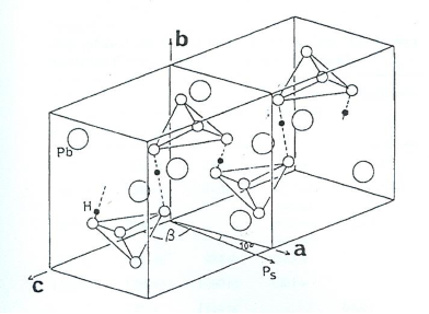
Figure 1: Unit cell of LHP crystal [23].

The second term in (2.1) is the Hamiltonian of short-range interactions between protons. The first Kronecker’s symbol corresponds to the proton interaction in the chain close to the tetrahedron of ‘A’-type, the second Kronecker’s symbol corresponds to proton interactions near the ‘B’-type tetrahedron, ${\bf r}$ is radius vector of the relative position of the proton bond in the unit cell. The quantity $w_{1}$ that describes short-range proton interactions within the chain may be expanded into a series with respect to deformations $\varepsilon_{i}$, $\varepsilon_{4}$ restricted to the linear summands [25]:

$$w_{1}=w+\sum\limits_{i=1}^{3}\delta_{i}\varepsilon_{i}+\delta_{4}\varepsilon_{4}\,.$$ (2.3)

The third term describes the effective long-range dipole-dipole interaction between protons within the chain running along $c$-axis, the fourth summand represents the lattice vibration energy ($b_{kl}^{+}$, $b_{kl}$ — Bose operators, ${l}$-index of phonon branch), the fifth summand corresponds to the proton-phonon interactions. The last term describes the interaction of the lattice with the external electrical field.

Long-range interactions of protons and interactions of protons with the lattice vibrations are considered within the the mean field approximation. Thus, the Hamiltonian (2.1) looks as follows:

$$\hat{H}=\hat{H}_{\textrm{p}}+\hat{H}_{\textrm{i}}\,,$$ (2.4)

where

$$\hat{H}_{\textrm{p}} = NvU_{1\textrm{seed}}-2w_{1}\sum\limits_{qq^{\prime}}\frac{\sigma_{q1}}{2}\frac{\sigma_{q2}}{2}\!\bigl{(}\delta_{{\bf R}_{q}{\bf R}_{q^{\prime}}}\!\!+\!\delta_{{\bf R}_{q}+{\bf r},{\bf R}_{q^{\prime}}}\bigr{)}$$ (2.5)

$$+\frac{1}{2}\sum\limits_{{qq^{\prime}},{ff^{\prime}}}J_{ff^{\prime}}(qq^{\prime})\frac{\langle\sigma_{qf}^{(n)}\rangle}{2}\frac{\langle\sigma_{q^{\prime}f^{\prime}}^{(n)}\rangle}{2}-\sum\limits_{{qq^{\prime}},{ff^{\prime}}}J_{ff^{\prime}}(qq^{\prime})\frac{\langle\sigma_{q^{\prime}f^{\prime}}^{(n)}\rangle}{2}\frac{\sigma_{qf}}{2}$$

$$+\frac{1}{\sqrt{N}}\sum\limits_{qf}\sum\limits_{kl}\tau_{lf}(\vec{k})\mathrm{e}^{\mathrm{i}\vec{k}\vec{a_{q}}}\langle b_{kl}+b_{-kl}^{+}\rangle\frac{\sigma_{qf}^{n}}{2}\,,$$

$$\hat{H}_{\textrm{i}} = \sum\limits_{kl}\omega_{l}(\vec{k})b_{kl}^{+}b_{kl}+\frac{1}{\sqrt{N}}\sum\limits_{qf}\sum\limits_{kl}\tau_{lf}(\vec{k})\mathrm{e}^{\mathrm{i}\vec{k}\vec{a_{q}}}\frac{\langle\sigma_{qf}\rangle}{2}\left(b_{kl}+b_{-kl}^{+}\right)$$ (2.6)

$$-\sum\limits_{q}\sum\limits_{kl}\left[\mu_{l}(\vec{k}){\rm cos}~{}5^{\circ}E_{1}^{\ast}+\mu_{l}(\vec{k}){\rm cos}~{}2^{\circ}E_{s}\right]\left(b_{kl}+b_{-kl}^{+}\right)\frac{1}{\sqrt{N}}\mathrm{e}^{\mathrm{i}\vec{k}\vec{a_{q}}}\,.$$

Using the Heisenberg equation of motion for the mean values of Bose-operators

$$\frac{\mathrm{d}}{\mathrm{d}t}\langle b_{kl}^{\pm}\rangle=-\mathrm{i}\langle[b_{kl}^{\pm},\widehat{H}]\rangle,$$ (2.7)

we find that

$$\langle b_{kl}+b_{-kl}^{+}\rangle = -\frac{1}{\sqrt{N}}\sum\limits_{q^{\prime}f^{\prime}}\frac{2\tau_{lf}(-\vec{k})}{\omega_{l}(\vec{k})}\mathrm{e}^{-\mathrm{i}\vec{k}\vec{a}_{q^{\prime}}}\frac{\sigma_{q^{\prime}f^{\prime}}}{2}$$ (2.8)

$$+\sum\limits_{q^{\prime}}\frac{2}{\omega_{l}(\vec{k})}\left[\mu_{l}(\vec{k}){\rm cos}~{}5^{\circ}E_{1}^{\ast}+\mu_{l}(\vec{k}){\rm cos}~{}2^{\circ}E_{s}\right]\frac{1}{\sqrt{N}}\mathrm{e}^{-\mathrm{i}\vec{k}\vec{a}_{q^{\prime}}}.$$

Taking into consideration the expression (2.5), the Hamiltonian of system $\hat{H}_{\textrm{p}}$ takes the following form:

$$\hat{H}_{\textrm{p}} = NvU_{1\textrm{seed}}-2w_{1}\sum\limits_{qq^{\prime}}\frac{\sigma_{q1}}{2}\frac{\sigma_{q2}}{2}\bigl{(}\delta_{{\bf R}_{q}{\bf R}_{q^{\prime}}}+\delta_{{\bf R}_{q}+{\bf r},{\bf R}_{q^{\prime}}}\bigr{)}$$

$$+\frac{1}{2}\sum\limits_{{qq^{\prime}},{ff^{\prime}}}\widetilde{J}_{ff^{\prime}}(qq^{\prime})\frac{\langle\sigma_{qf}\rangle}{2}\frac{\langle\sigma_{q^{\prime}f^{\prime}}\rangle}{2}-\sum\limits_{{qq^{\prime}},{ff^{\prime}}}\widetilde{J}_{ff^{\prime}}(qq^{\prime})\frac{\langle\sigma_{q^{\prime}f^{\prime}}\rangle}{2}\frac{\sigma_{qf}}{2}$$

$$-\sum\limits_{q}\left[\mu{\rm cos}~{}5^{\circ}E_{1}^{\ast}+\mu{\rm cos}~{}2^{\circ}E_{s}\right]\left(\frac{\sigma_{q1}}{2}+\frac{\sigma_{q2}}{2}\right).$$

The following notations are used herein:

$$\widetilde{J}_{ff^{\prime}}(qq^{\prime}) = J_{ff^{\prime}}(qq^{\prime})+\frac{1}{{N}}\sum\limits_{kl}\frac{2\tau_{lf}(\vec{k})\tau_{lf^{\prime}}(-\vec{k})}{\omega_{l}(\vec{k})}\mathrm{e}^{\mathrm{i}\vec{k}(\vec{a}_{q}-\vec{a}_{q^{\prime}})},$$ (2.9)

$$\mu = \sum\limits_{q^{\prime}}\sum\limits_{kl}\mu_{il}(\vec{k})\frac{\tau_{lf}(\vec{k})}{\omega_{l}(\vec{k})}\frac{1}{\sqrt{N}}\mathrm{e}^{\mathrm{i}\vec{k}(\vec{a_{q}}-\vec{a}_{q^{\prime}})}.$$ (2.10)

Considering the symmetry of unary function of proton distribution

$$\eta^{(1)x}=\langle\sigma_{q1}\rangle=\langle\sigma_{q2}\rangle$$

and expanding the constant of long-range proton-proton interactions into a series with respect to deformations $\varepsilon_{i}$, $\varepsilon_{4}$, restricted to the linear summands:

$$J_{ff^{\prime}}=J+\sum\limits_{i=1}^{3}\psi_{1i}\varepsilon_{i}+\psi_{4}\varepsilon_{4}\,,$$ (2.11)

where $J_{ff^{\prime}}=\sum_{{\bf R}_{q}-{\bf R}_{q^{\prime}}}J_{ff^{\prime}}(qq^{\prime})$ are Fourier transforms of the constants of long-range interaction, we get an output Hamiltonian $\hat{H}$ in the following form:

$$\hat{H} = NvU_{1\textrm{seed}}-2w_{1}\sum\limits_{qq^{\prime}}\frac{\sigma_{q1}}{2}\frac{\sigma_{q2}}{2}\bigl{(}\delta_{{\bf R}_{q}{\bf R}_{q^{\prime}}}+\delta_{{\bf R}_{q}+{\bf r},{\bf R}_{q^{\prime}}}\bigr{)}-2N\nu_{1}(\eta^{(1)x})^{2}-2\nu_{1}\eta^{(1)x}\left(\frac{\sigma_{q1}}{2}+\frac{\sigma_{q2}}{2}\right)$$ (2.12)

$$-\sum\limits_{q}\mu_{s}E_{s}\left(\frac{\sigma_{q1}}{2}+\frac{\sigma_{q2}}{2}\right)-\sum\limits_{q}\mu_{1}^{\ast}E_{1}^{\ast}\left(\frac{\sigma_{q1}}{2}+\frac{\sigma_{q2}}{2}\right),$$

where the following notations are used:

$$\nu_{1}=\nu+\sum\limits_{i}\psi_{i}\varepsilon_{i}+\psi_{4}\varepsilon_{4}\,,\qquad\nu=\frac{J}{2}\,,\qquad\mu_{1}^{\ast}=\mu{\rm cos}~{}5^{\circ},\qquad\mu_{s}=\mu{\rm cos}~{}2^{\circ}.$$

The approximation of two-particle cluster is used in order to calculate the physical characteristics of PbHPO₄-type compound. In this approximation, the LHP thermodynamic potential is as follows:

$$G_{1} = NU_{1\textrm{seed}}+2N\nu_{1}(\eta^{(1)x})^{2}-k_{\textrm{B}}T\sum\limits_{q}\left\{\ln{\rm Sp}\mathrm{e}^{-\beta\hat{H}^{(2)}_{qA}}+\ln{\rm Sp}\mathrm{e}^{-\beta\hat{H}^{(2)}_{qB}}-\frac{1}{2}\ln{\rm Sp}\mathrm{e}^{-\beta\hat{H}^{(1)}_{q}}\right\}$$ (2.13)

$$-Nv\sum\limits_{i}\sigma_{i}\varepsilon_{i}-Nv\sigma_{4}\varepsilon_{4}\,,$$

where $\hat{H}^{(2)}_{q{A(B)}}$, $\hat{H}^{(1)}_{q}$ are two-particle and one-particle Hamiltonians assigned by the following equations:

$$\hat{H}^{(2)}_{qA}=-2w_{1}\left(\frac{\sigma_{q1}}{2}\frac{\sigma_{q2}}{2}\right)-\frac{x_{E}}{\beta}\left(\frac{\sigma_{q1}}{2}+\frac{\sigma_{q2}}{2}\right),$$ (2.14)

$$\hat{H}^{(1)}_{q}=-\frac{\bar{x}_{E}}{\beta}\frac{\sigma_{qf}^{(1)}}{2}\,.$$ (2.15)

The following notations are used herein:

$$x_{E}=\beta\left(-\Delta^{a}+2\nu_{1}\eta^{(1)x}+\mu_{1}^{\ast}E_{1}^{\ast}+\mu_{s}E_{s}\right),\qquad\bar{x}_{E}=-\beta\Delta^{a}+x_{E},\qquad\beta=1/k_{\textrm{B}}T,$$ (2.16)

where $\Delta^{a}$ is the effective field formed dy the neighboring links beyond the cluster borders. Within the cluster approximation, the $\Delta^{a}$ field is determined according to the condition of self-consistency, i.e., the mean value of pseudospin $\langle\sigma_{qf}^{(l)x}\rangle$ should not depend on a particular Gibbs distribution (two-particle or one-particle Hamiltonian) according to which it is estimated:

$$\frac{{\rm Sp}\,\sigma_{qf}^{(l)}\mathrm{e}^{-\beta\hat{H}^{(2)}_{qA}}}{{\rm Sp}\,\mathrm{e}^{-\beta\hat{H}^{(2)}_{qA}}}=\frac{{\rm Sp}\,\sigma_{qf}^{(l)}\mathrm{e}^{-\beta\hat{H}^{(1)}_{q}}}{{\rm Sp}\,\mathrm{e}^{-\beta\hat{H}^{(1)}_{q}}}\,.$$ (2.17)

Then, based on (2.17) and considering (2.14) and (2.15), we get an equation for the mean value of pseudospin in the following form:

$$\eta^{(1)x}=\frac{{\sinh}x_{E}}{a_{1}+{\cosh}x_{E}}=\frac{{\sinh}x_{E}}{D}\,,$$ (2.18)

where

$$x_{E}=\frac{1}{2}\ln\frac{1+\eta^{(1)x}}{1-\eta^{(1)x}}+\beta\nu_{1}\eta^{(1)x}+\frac{\beta\mu_{1}^{\ast}E_{1}^{\ast}}{2}+\frac{\beta\mu_{s}E_{s}}{2}\,,\qquad a_{1}=\exp\left[{-\beta\left(w+\sum\limits_{i=1}^{3}\delta_{i}\varepsilon_{i}+\delta_{4}\varepsilon_{4}\right)}\right].$$

3 Static dielectric, piezoelectric, elastic and thermal characteristics
of PbHPO₄

Having calculated the eigenvalues of two-particle and one-particle Hamiltonians, let us present the thermodynamic potential (2.13) per unit cell in the following form:

$$g_{1} = \frac{G_{1}}{N}=vU_{1\textrm{seed}}-2k_{\textrm{B}}T\ln 2-(w+\delta_{1}\varepsilon_{1}+\delta_{2}\varepsilon_{2}+\delta_{3}\varepsilon_{3}+\delta_{5}\varepsilon_{5})$$

$$+\bigl{(}\nu+\psi_{1}\varepsilon_{1}+\psi_{2}\varepsilon_{2}+\psi_{3}\varepsilon_{3}+\psi_{4}\varepsilon_{4}\bigr{)}(\eta^{(1)x})^{2}$$

$$-\,k_{\textrm{B}}T\ln\left[1-(\eta^{(1)x})^{2}\right]-2k_{\textrm{B}}T\ln(a_{1}+{\cosh}x_{E})-v(\sigma_{1}\varepsilon_{1}+\sigma_{2}\varepsilon_{2}+\sigma_{3}\varepsilon_{3})-v\sigma_{4}\varepsilon_{4}\,.$$

Using the equilibrium equation

$$\frac{1}{v}\left(\frac{\partial g_{1}}{\partial\varepsilon_{i}}\right)_{E_{1}}=0,\qquad\frac{1}{v}\left(\frac{\partial g_{1}}{\partial E_{1}}\right)_{\varepsilon_{i}}=-P_{1}\,,\qquad\frac{1}{v}\left(\frac{\partial g_{1}}{\partial E_{1}^{\ast}}\right)_{\varepsilon_{i}}=-P_{1}^{\ast}\,,$$

we get an equation for deformation $\varepsilon_{i}$, $\varepsilon_{4}$ and polarization $P_{1}$:

$$0=c_{i1}^{E0}\varepsilon_{1}+c_{i2}^{E0}\varepsilon_{2}+c_{i3}^{E0}\varepsilon_{3}+c_{i4}^{E0}\varepsilon_{4}-e_{1i}^{0}E_{1}-\frac{\delta_{i}}{v}\frac{{\cosh}x-a_{1}}{a_{1}+{\cosh}x}-\frac{\psi_{i}}{v}(\eta^{(1)x})^{2},$$ (3.1)

$$0=c_{14}^{E0}\varepsilon_{1}+c_{24}^{E0}\varepsilon_{2}+c_{34}^{E0}\varepsilon_{3}+c_{44}^{E0}\varepsilon_{4}-e_{14}^{0}E_{1}-\frac{\delta_{4}}{v}\frac{{\cosh}x-a_{1}}{a_{1}+{\cosh}x}-\frac{\psi_{4}}{v}(\eta^{(1)x})^{2},$$ (3.2)

$$P_{1}^{\ast}=\chi_{11}^{\ast\varepsilon 0}E_{1}^{\ast}+\frac{\mu_{1}^{\ast}}{v}\eta^{(1)x},$$ (3.3)

$$P_{\textrm{s}}=\frac{\mu_{s}}{v}\eta^{(1)x}.$$ (3.4)

Based on the relation (3.1) and (3.4), we get the following thermodynamic characteristics of LHP crystals, i.e., isothermal static susceptibility of a mechanically clamped crystal:

$$\chi_{11}^{{}^{\ast}\varepsilon T}=\left(\frac{\partial P_{1}^{\ast}}{\partial E_{1}^{\ast}}\right)_{\varepsilon_{i}}=\chi_{11}^{\varepsilon 0}+\frac{(\mu_{1}^{\ast})^{2}}{2v}\frac{\beta\varkappa_{E}}{D-\varkappa_{E}\varphi^{\eta}}\,,$$ (3.5)

where the following notations are used:

$$\varkappa_{E}={\cosh}x_{E}-\eta^{(1)x}{\sinh}x_{E},\qquad\varphi^{\eta}=\frac{1}{1-(\eta^{(1)x})^{2}}+\beta\nu_{1};$$

isothermal coefficients of piezoelectric stress:

$$e_{1i}^{T}=\left(\frac{\partial P_{1}}{\partial\varepsilon_{i}}\right)_{E_{1}}=e_{1i}^{0}+\frac{\mu_{1}}{v}\frac{\beta(\psi_{i}\varkappa+\delta_{i}a_{1})}{D-\varkappa\varphi^{\eta}}\eta^{(1)},\qquad e_{14}^{T}=\left(\frac{\partial P_{1}}{\partial\varepsilon_{4}}\right)_{E_{1}}=e_{14}^{0}+\frac{\mu_{1}}{v}\frac{\beta(\psi_{4}\varkappa+\delta_{4}a_{1})}{D-\varkappa\varphi^{\eta}}\eta^{(1)};$$

isothermal elastic constants at a constant field:

$$c_{ij}^{E} =\left(\frac{\partial\sigma_{i}}{\partial\varepsilon_{i}}\right)_{E_{1}}=c_{ij}^{E0}-\frac{\beta}{v}\delta_{i}\delta_{j}\frac{a_{1}{\cosh}x}{D^{2}}-\frac{\beta}{v}\frac{\eta^{(1)2}}{D-\varkappa\varphi^{\eta}}\left[\delta_{i}\delta_{j}\frac{\varphi^{\eta}a_{1}^{2}}{D}+\psi_{i}\psi_{j}\varkappa+\bigl{(}\delta_{i}\psi_{j}+\delta_{j}\psi_{i}\bigr{)}a_{1}\right],$$

$$c_{i4}^{E} =c_{i5}^{E0}-\frac{\beta\delta_{1}\delta_{4}{\cosh}x}{vD^{2}}-\frac{\beta\eta^{(1)2}}{v\bigl{(}D-\varkappa\varphi^{\eta}\bigr{)}}\left[\delta_{i}\delta_{4}\frac{a_{1}^{2}\varphi^{\eta}}{D}+\psi_{i}\psi_{4}\varkappa+\bigl{(}\delta_{i}\psi_{4}+\psi_{i}\delta_{4}\bigr{)}a_{1}\right],$$

$$c_{44}^{E0} =c_{44}^{E0}-\frac{\beta\delta_{4}^{2}{\cosh}x}{vD^{2}}-\frac{\beta\eta^{(1)2}}{v\bigl{(}D-\varkappa\varphi^{\eta}\bigr{)}}\left[\delta_{4}^{2}\frac{a_{1}^{2}\varphi^{\eta}}{D}+\psi_{4}^{2}\varkappa+2\delta_{4}\psi_{4}a_{1}\right].$$

Other dielectric, piezoelectric and elastic characteristics of LHP may be calculated using the above mentioned results. In particular, we may get the matrix of isothermal compliance at a static field $s_{ij}^{E}$, which is inverse to the matrix of elastic constant $c_{ij}^{E}$; isothermal coefficients of the piezoelectric strain:

$$d_{1i}^{T}=\sum\limits_{j}s_{ij}^{E}e_{1i}^{T}\,,\qquad(i,j=1,2,3,4),$$ (3.6)

isothermal dielectric susceptibility of free crystals:

$$\chi_{11}^{\sigma T}=\chi_{11}^{\varepsilon T}+\sum\limits_{i}e_{1i}^{T}d_{1i}^{T}\,.$$ (3.7)

In the LHP crystals, there takes phase a phase transition of the second order from paraelectric phase into ferroelectric phase at temperature that satisfies the equation:

$$\exp\left(-\frac{w_{1}}{k_{\textrm{B}}T_{\textrm{c}}}\right)=\frac{\nu_{1}}{k_{\textrm{B}}T_{\textrm{c}}}\,.$$ (3.8)

The molar entropy of a crystal conditioned by a proton subsystem is obtained through a direct differentiation of thermodynamic potential:

$$S=-\frac{R}{2}\left(\frac{\mathrm{d}g_{1}}{\mathrm{d}T}\right)_{\sigma_{i}}=\frac{R}{2}\left\{\ln 2+\ln\left[1-(\eta^{(1)})^{2}\right]+2\ln D-2\beta\nu_{1}(\eta^{(1)})^{2}+\frac{2\beta w_{1}}{D}a_{1}\right\},$$ (3.9)

where $R$ is a universal gas constant.

The molar heat capacity of a hydrogen subsystem of LHP at a constant strain is calculated by a direct differentiation of entropy (3.9):

$$\Delta C_{\textrm{p}} = T\left(\frac{\partial S}{\partial T}\right)_{\sigma}$$

$$= T\left(\frac{\partial S}{\partial T}\right)_{\eta,\varepsilon}+T\left(\frac{\partial S}{\partial\eta}\right)_{\varepsilon}\left(\frac{\mathrm{d}\eta}{\mathrm{d}T}\right)+\sum\limits_{i=1}^{3}T\left(\frac{\partial S}{\partial\varepsilon_{i}}\right)_{\eta}\left(\frac{\mathrm{d}\varepsilon_{i}}{\mathrm{d}T}\right)+T\left(\frac{\partial S}{\partial\varepsilon_{4}}\right)_{\eta}\left(\frac{\mathrm{d}\varepsilon_{4}}{\mathrm{d}T}\right).$$

4 Relaxational dynamics of PbHPO₄ crystal

This section describes the dynamic phenomena in LHP at the application of electrical field $E_{1}^{\ast}$ to a crystal. While calculating the dynamic characteristic of this kind of ferroelectrics we use a kinetic equation [26, 28, 27] based on the method of non-equilibrium statistical Zubarev operator [29].

The kinetic equation for the mean values of pseudospin operator is as follows:

$$\frac{\mathrm{d}}{\mathrm{d}t}\langle\hat{p}_{m}\rangle=-\sum\limits_{qf}\sum\limits_{\mu\alpha}\left[Q_{qf\mu\alpha}^{-}(\hat{p}_{m})+{\tanh}\frac{\beta\Omega_{\mu}^{\alpha}}{2}Q_{qf\mu\alpha}^{+}(\hat{p}_{m})\right]K_{\mu}^{\alpha}\,,$$ (4.1)

where

$$Q_{qf\mu\alpha}^{\mp}(\hat{p}_{m})=\langle\left\{[\hat{p}_{m},\sigma_{qf}^{-\alpha}\bigl{(}\Omega_{\mu}^{\alpha^{\prime}}\bigr{)}],\sigma_{qf}^{\alpha}\bigl{(}\Omega_{\mu}^{\alpha}\bigr{)}\right\}^{\mp}\rangle_{q}\,,$$ (4.2)

$$K_{\mu}^{\alpha}=\int\limits_{0}^{\infty}dte^{-\varepsilon t}\cos\Omega_{\mu}^{\alpha}t{\rm Re}\langle\bar{u}(t)\bar{u}^{+}\rangle_{q}\,,\qquad\alpha=0,\pm 1,$$ (4.3)

while $\langle\bar{u}^{\alpha}(t)\bar{u}^{\alpha^{\prime}}\rangle_{q}$ are correlation function of a thermostat, $\sigma_{qf}^{\alpha}\bigl{(}\Omega_{\mu}^{\alpha}\bigr{)}$ is a Fourier component of the operator $\sigma_{qf}^{\alpha}(t)$, $\Omega_{\mu}^{\alpha}$ are eigenfrequencies of the Hamiltonian of pseudo-spin model (2.14), $\sigma_{qf}^{0}=\sigma_{qf}$, $\sigma_{qf}^{\pm}=\sigma_{qf}^{x}\pm\mathrm{i}\sigma_{qf}^{y}$.

Taking into account the time evolution law of pseudo-spin operators $\sigma_{qf}^{\alpha}(t)$ and using the frequency presentation of these operators, one may calculate the expressions for $Q_{qf\mu\alpha}^{\mp}\bigl{(}\hat{p}_{qf}\bigr{)}$ in another form. Finally, it allows us to rewrite the kinetic equation (4.1) as follows:

$$\frac{\mathrm{d}}{\mathrm{d}t}\eta^{(1)x}=b_{11}\eta^{(1)x}+b_{12}\eta^{(2)x}+b_{1}\,,$$ (4.4)

$$\frac{\mathrm{d}}{\mathrm{d}t}\eta^{(2)x}=b_{21}\eta^{(1)x}+b_{22}\eta^{(2)x}+b_{2}\,,$$

as well as the equation for a unary function in one-frequency approximation:

$$\frac{\mathrm{d}}{\mathrm{d}t}\eta^{(1)x}=-2K_{0}\eta^{(1)x}+2K_{0}{\tanh}\frac{\beta\Omega_{0}}{2}\,.$$ (4.5)

The following notations are used herein:

$$b_{11}=-(K_{1}+K_{-1})+K_{1}Z_{1}-K_{-1}Z_{-1}\,, b_{12}=-K_{1}+K_{-1}\,, b_{1}=K_{1}Z_{1}+K_{-1}Z_{-1}\,,$$

$$b_{21}=-2(K_{1}-K_{-1})+2(K_{1}Z_{1}+K_{-1}Z_{-1})\,, b_{22}=-2(K_{1}+K_{-1})\,, b_{2}=2(K_{1}Z_{1}-K_{-1}Z_{-1})\,,$$

$$K_{\mu}=K_{\mu}^{-1}+K_{\mu}^{1}=\int\limits_{0}^{\infty}\mathrm{d}t\mathrm{e}^{-\varepsilon t}\cos\bigl{(}\Omega_{\mu}t\bigr{)}{\rm Re}\left\{\langle\bar{u}^{-}(t)\bar{u}^{+}\rangle_{q}+\langle\bar{u}^{+}(t)\bar{u}^{-}\rangle_{q}\right\},\qquad Z_{\mu}={\tanh}\frac{\beta\Omega_{\mu}}{2}.$$

In case $K_{0}=K_{-1}=K_{1}={1}/{2\alpha}$, the system equations obtained in this section are in agreement with the equations obtained within the framework of a stochastic Glauber model [30]. Glauber equations describe a physical situation at which the Fourier images of the thermostat correlators are independent of the frequency [28, 26].

Thus, from equations (4.4) and (4.5), we find that

$$\alpha\frac{\mathrm{d}}{\mathrm{d}t}\eta^{(1)x}=-(1-P)\eta_{s}^{(1)x}+L,$$ (4.6)

$$\alpha\frac{\mathrm{d}}{\mathrm{d}t}\eta^{(1)x}=-\eta^{(1)x}+{\tanh}\frac{\bar{x}}{2}\,,$$

where the following notation is used:

$$P=\frac{1}{2}\left[{\tanh}\left(\frac{\beta w_{1}}{2}+\frac{x_{E}}{2}\right)-{\tanh}\left(-\frac{\beta w_{1}}{2}+\frac{x_{E}}{2}\right)\right],$$

$$L=\frac{1}{2}\left[{\tanh}\left(\frac{\beta w_{1}}{2}+\frac{x_{E}}{2}\right)+{\tanh}\left(-\frac{\beta w_{1}}{2}+\frac{x_{E}}{2}\right)\right].$$ (4.7)

Solving equations (4.6) in the case of small deviations from the equilibrium state, one may obtain the complex dielectric permittivity of the hydrogen subsystem of LHP:

$$\varepsilon_{11}^{\prime\ast}(\omega)=\varepsilon_{11}^{\varepsilon 0}+\frac{4\pi\chi^{\ast}}{1+(2\pi\nu\tau)^{2}}\,,\qquad\varepsilon_{11}^{\prime\prime\ast}(\omega)=\ \frac{4\pi\chi^{\ast}\pi\nu\tau}{1+(2\pi\nu\tau)^{2}}$$ (4.8)

with the set of following notations

$$\chi^{\ast} =\frac{\mu_{1}^{\ast 2}\beta}{2v}\left\{\frac{2r\left[1-P^{(0)}\right]-Y}{Yr}-\beta\left(\nu+\nu_{ab}\right)\right\}^{-1}\,$$

$$\tau^{-1} =\frac{1}{\alpha}\frac{Yr}{2r-Y}\left\{\frac{2r\left[1-P^{(0)}\right]-Y}{Yr}-\beta(\nu+\nu_{ab})\right\},$$

$$Y =P^{(1)}\eta^{(1)}+L^{(1)},\qquad r=1-\bigl{(}\eta^{(1)}\bigr{)}^{2},$$

$$P^{(0)} =\frac{1-a_{1}^{2}}{1+a_{1}^{2}+2a_{1}{\cosh}{x}}\,, L^{(0)} =\frac{2a_{1}{\sinh}{x}}{1+a_{1}^{2}+2a_{1}{\cosh}{x}}\,,$$

$$P^{(1)} =-\frac{4a_{1}(1-a1^{2}){\sinh}{x}}{[1+a_{1}^{2}+2a_{1}{\cosh}{x}]^{2}}\,, L^{(1)} =\frac{4a_{1}[2a_{1}+(1+a_{1}^{2}){\cosh}{x}]}{[1+a_{1}^{2}+2a_{1}{\cosh}{x}]^{2}}\,.$$

5 Comparison of numerical calculations with experimental data.
Discussion of the results obtained

Prior to the discussion of the developed theory, it should be noted that this theory, strictly speaking, holds for deuterated ferroelectric LDP. Thermodynamic and dynamic characteristics of hydrogen-bonded ferroelectrics taking tunneling $\Omega$ into account, are essentially defined by an effective parameter of tunneling $\bar{\Omega}$, which is renormalized by short-range interactions [31]. Here, $\bar{\Omega}\ll\Omega$, i.e., an essential suppression of tunneling by short-range interactions takes place. Then, let us assume that the theory proposed by us holds for LHP crystals as well taking into consideration, in particular, the relaxational type of dispersion in LHP.

Unfortunately, the elastic constants of the LHP crystal have not been experimentally determined so far. That is why it is impossible to specify the seed elastic constants and hence to calculate, based on the proposed theory, the piezoelectric coefficients, susceptibility of a mechanically free crystal, elastic constants in ferroelectric phase. In order to perform the numerical calculations of temperature and frequency dependencies of respective physical characteristics of LHP, the values of the following parameters should be specified:

• parameter of a two-particle cluster $w$;

• parameter of long-range interaction $\nu$ ;

• effective dipole moment $\mu_{s}$;

• the seed dielectric susceptibilities $\chi_{11}^{0}$;

• parameter $\alpha$ that defines the time scale of relaxation processes.

In order to determine the above mentioned parameters, let us use temperature dependencies of experimental physical characteristics, namely $T_{\textrm{c}}$, $P_{s}(T)$ [1], $\varepsilon_{11}(0,T)$ [1]. The value of the effective dipole moment $\mu_{s}$ is determined through the agreement of the theory with the experiment for polarization of saturation. In paraelectric phase, we determine $\mu_{1+}^{\ast}$ by agreeing the theory with the experiment for $\varepsilon_{11}^{\sigma}(T)$.

Table 1: A set of parameters of the theory for LHP and LDP crystals.

	$T_{\textrm{c}}$	${w}/{k_{\textrm{B}}}$	${\nu}/{k_{\textrm{B}}}$	$\mu_{\textrm{s}}$, $10^{-18}$	$\mu_{1\textrm{p}}^{\ast}$, $10^{-18}$	$\chi_{11}^{\varepsilon 0}$	$P_{\textrm{s}}$	$R_{\textrm{s}}$	$P_{\textrm{p}}$	$R_{\textrm{p}}$
	(K)	(K)	(K)	($\text{esu}\cdot\text{cm}$)	($\text{esu}\cdot\text{cm}$)		(s)	(s/K)	(s)	(s/K)
PbHPO4	310	850	19.98	1.00	1.46	0.716	0.339	-0.009	0.745	0.002
PbDPO4	452	1450	2.19	1.05	2.00	0.716

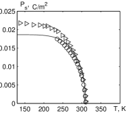
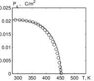
Figure 2: Temperature dependencies of spontaneous polarization of LHP — $\circ$ [1], $\diamond$ [7] and LDP — $\circ$ [1].

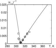
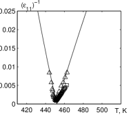
Figure 3: Temperature dependencies of dielectric permittivities of LHP — $\circ$ [1], $\square$ [32], $\vartriangle$ [33] and LDP — $\vartriangle$ [13], $\square$ [32].

Figure 4: Temperature dependence of heat capacity for LHP crystal: $\ast$, [9].

Parameter $\alpha$ is defined from the condition that theoretically calculated curves of $\varepsilon_{11}(\omega)$ should agree with the experimentally obtained curves. In is assumed that parameter $\alpha$ slightly changes with temperature:

$$\alpha=[P+R(\Delta T)]\cdot 10^{-14},\qquad\Delta T=T-T_{\textrm{c}}\,.$$

The unit cell volume of LHP is taken to be equal to $v=0.1788\cdot 10^{-21}$ cm³, LDP — $v=0.1800\cdot 10^{-21}$ cm³.

The set of optimal parameters obtained this way is presented in table 1.

Let us now discuss the obtained results. Figure 2 shows temperature dependencies of spontaneous polarization of LHP and LDP crystals together with the experimental data. It is seen in the figure that the data in papers [1] and [7] disagree between themselves. There is a good description of temperature dependencies of spontaneous polarization obtained in paper [1]. Polarization of saturation increases at the growth of the degree of deuteration $x$.

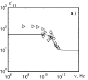
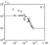
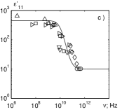
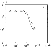
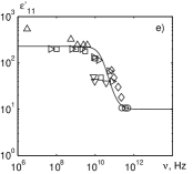
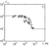
Figure 5: Frequency dependencies of real $\varepsilon^{\prime}_{11}$ part of dielectric permittivity of LHP at $\Delta T$: a) $-10$ K; b) $-5$ K; c) 5 K; d) 7.16 K; e) 10 K; f) 20 K and experimental data: $\Box$ — [32], $\diamond$ — [34], $\circ$ — [5], $\bigtriangledown$ — [35]; $\triangleright$ — [36], $\bigtriangleup$ — [37].

Figure 6: Frequency dependencies of imaginary $\varepsilon^{\prime\prime}_{11}$ part of dielectric permittivity of LHP at $\Delta T$: a) $-10$ K; b) $-5$ K; c) 5 K; d) 7.16 K; e) 10 K; f) 20 K and experimental data: $\Box$ — [32], $\diamond$ — [34]; $\circ$ — [5]; $\bigtriangledown$ — [35]; $\triangleright$ — [36], $\bigtriangleup$ — [37].

Figure 3 presents temperature dependencies of static dielectric permittivities of mechanically clamped $\varepsilon_{11}^{\ast}(0,T)$ crystals of LHP and LDP calculated based on the microscopic theory, as well as the results of experimental studies [1, 7, 33].

As it is seen in figure 3, the results of theoretical calculations of $\varepsilon_{11}^{\ast}(0,T)$ on the whole show good quantitative agreement with experimental data obtained by the authors [1, 32, 33].

The temperature dependence of heat capacity for LHP crystal, together with experimental data of paper [9] are presented in figure 4.

The dashed line shows the effective lattice contribution $C_{0}$ into the heat capacity which is estimated by us as the average of the difference $C_{\textrm{p}}(T)-\Delta C_{\textrm{p}}(T)$. Based on the proposed model and using the theory parameters (table 1), a quantitatively good description of the data of paper [9] has been achieved. The amount of the calculated heat capacity jump well correlates with the experiment.

The measured temperature dependencies of a real and imaginary parts of dielectric permittivity at different frequencies for LHP are presented in papers [5, 34, 35, 36, 37, 32, 38].

Figures 5 and 6 present the results of calculations of frequency dependencies $\varepsilon^{\prime}_{11}(\nu)$ and $\varepsilon^{\prime\prime}_{11}(\nu)$, respectively, for LHP as well as experimental data.

In these figures it is seen that there is a significant data scattering obtained in the experimental papers [5, 34, 35, 36, 37, 32]. The best agreement for our calculated data of $\varepsilon^{\prime}_{11}(\nu)$ and $\varepsilon^{\prime\prime}_{11}(\nu)$ and the experiment was reached with the results published in papers [32, 34, 5].

Figure 7 presents temperature dependencies of real $\varepsilon_{11}^{\prime}(\nu,T)$ and imaginary $\varepsilon_{11}^{\prime\prime}(\nu,T)$ parts of dynamic dielectric permittivity at different frequencies of LHP crystal as well as the experimental data.

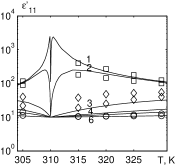
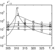
Figure 7: Temperature dependencies of real $\varepsilon_{11}^{\prime}(\nu,T)$ and imaginary $\varepsilon_{11}^{\prime\prime}(\nu,T)$ parts of dielectric permittivity of LHP crystal at different frequencies $\nu$ (GHz): 1 — 1, $\square$ [32]; 10 — 2, $\square$ [32]; 94 — 3; $\lozenge$ [34]; 179 — 4, $\lozenge$ [34]; 240 — 5, $\circ$ [5]; 480 — 6, $\circ$ [5].

As seen in this figure, there is quite acceptable agreement between our theoretical results and the majority of experimental data. A significant disagreement is observed only with the experimental data of Briskot et al. [34]. The reason is a rather poor experimental accuracy (order of 40–50 %) of their experimental setup.

6 Conclusions

The present paper, based on a modified model of proton ordering that does not take into consideration the proton tunneling on hydrogen bonds in the approximation of a two-particle cluster, describes the theory of thermodynamic and dielectric, piezoelectric, elastic and dynamic properties of one-dimentional ferroelectrics of PbHPO₄-type. Optimal sets of model parameters have been found that make it possible to describe the available corresponding experimental data for LHP and LDP crystals.

Ukrainian 0 Термодинамiчнi та динамiчнi дiелектричнi властивостi одновимiрних сегнетоелектрикiв з водневими зв’язками типу PbHPO₄ I.Р. Зачек${}^{\textsf{\footnotesize{\mbox{?}}}}$, Р.Р. Левицький${}^{\textsf{\footnotesize{\mbox{?}}}}$, Я.Й. Щур${}^{\textsf{\footnotesize{\mbox{?}}}}$, О.Б. Бiленька${}^{\textsf{\footnotesize{\mbox{?}}}}$

             
${}^{\textsf{\footnotesize 1}}$ Iнститут фiзики конденсованих систем НАН України, вул. I Свєнцiцького, 1, 79011 Львiв, Україна ${}^{\textsf{\footnotesize 2}}$ Нацiональний унiверситет ‘‘Львiвська полiтехнiка’’, вул. С. Бандери, 12, 79013 Львiв, Україна

References

• [1] Negran T.J., Glass A.M., Brickenkamp C.S., Rosenstein R.D., Osterheld R.K., Susott R., Ferroelectrics, 1974, 6, 179; doi:10.1080/00150197408243964.
• [2] Nelmes R.J., Choudhary R.N.P., Ferroelectrics, 1978, 21, 467; doi:10.1080/00150197808237299.
• [3] Blinc R., Arend H., Kanduser A., Phys. Status Solidi B, 1976, 74, No. 2, 425; doi:10.1002/pssb.2220740202.
• [4] Levrenčič B.B., Čopič M., Zgonik M., Petzelt J., Ferroelectrics, 1978, 21, 325; doi:10.1080/00150197808237254.
• [5] Kroupa J., Petzelt J., Kozlov G.V., Volkov A.A., Ferroelectrics, 1978, 21, 367; doi:10.1080/00150197808237273.
• [6] Březina B., Smutný F., Fosek J., Czech. J. Phys. B, 1975, 25, 1411; doi:10.1007/BF01587566.
• [7] Smutný F., Fousek J., Ferroelectrics, 1978, 21, 385; doi:10.1080/00150197808237272.
• [8] Fouskova A., Březina B., Ferroelectrics, 1978, 19, 119; doi:10.1080/00150197808237839.
• [9] López-Echarri A., Tello M.J., Jubindo M.A., Solid State Commun., 1981, 38, 383;
doi:10.1016/0038-1098(81)90262-3.
• [10] Shchur Ya., Phys. Status Solidi B, 2009, 246, 102; doi:10.1002/pssb.200844321.
• [11] Shchur Ya., Phase Transitions, 2013, 86, 857; doi:10.1080/01411594.2012.745539.
• [12] Bajpai P.K., Choudhary R.N.P., Ferroelectrics, 1999, 234, 29; doi:10.1080/00150199908225279.
• [13] De Carvalho A.V., Salinas S.R., J. Phys. Soc. Jpn., 1978, 44, No. 1, 238; doi:10.1143/JPSJ.44.238.
• [14] Chaudhuri B.K., Ganguli S., Nath D., Phys. Rev. B, 1981, 23, No.5, 2308; doi:10.1103/PhysRevB.23.2308.
• [15] Blinc R., Arend H., Phys. Status Solidi B, 1976, 74, 425; doi:10.1002/pssb.2220740202.
• [16] Zinenko V.I., Fiz. Tverd. Tela, 1979, 21, No. 6, 1819 (in Russian).
• [17] Korinevskii N.A., In: Physics of Many-Particle Systems, Kiev, Naukova dumka, 1983, No. 4, 84.
• [18] Wesselinowa J.M., J. Phys.: Condens. Matter, 1991, 3, 4757; doi:10.1088/0953-8984/3/25/022.
• [19] Upadhyay T.C., Mayank Joshi, J. Metall. Mater. Sci., 2012, 54, 209.
• [20] Blinc R., Žeks B., Sampaio J.F., Pires A.S.T., SaBarreto F.C., Phys. Rev. B, 1979, 20, No. 5, 1991;
doi:10.1103/PhysRevB.20.1991.
• [21] Levitskii R.R., Sorokov S.I., Preprint of the Institute for Theoretical Physics, ITF-78-152P, Kyiv, 1978 (in Russian).
• [22] Levitskii R.R., Zachek I.R., Vdovych A.S., Phys. Chem. Solid State, 2012, 13, 40 (in Ukrainian).
• [23] Pasquier B., Fillaux F., Tomkinson J., Physica B, 1995, 213, 658; doi:10.1016/0921-4526(95)00241-Z.
• [24] Stasyuk I.V., Levitskii R.R., Ukr. Fiz. Zh., 1970, 15, 460 (in Russian).
• [25] Levitskii R.R., Zachek I.R., Vdovych A.S., Stasyuk I.V., J. Phys. Stud., 2013, 17, 4703.
• [26] Berim G.O., Kessel A.R., Physica A, 1980, 101, No. 1, 112; doi:10.1016/0378-4371(80)90103-X.
• [27] Levitskii R.R., Zachek I.R., Sokolovskii R.O., Condens. Matter Phys., 1998, 1, No. 4, 849; doi:10.5488/CMP.1.4.849.
• [28] Berim G.O., Kessel A.R., Physica A, 1980, 101, No. 1, 127; doi:10.1016/0378-4371(80)90104-1.
• [29] Zubarev D.N., Nonequilibrium Statistical Thermodynamics, Consultants Bureau, New York, 1974.
• [30] Glauber J., J. Math. Phys., 1963, 4, No. 2, 294; doi:10.1063/1.1703954.
• [31] Yukhnovskii I.R., Levitskii R.R., Sorokov S.I., Derzhko O.V., Izv. Akad. Nauk SSSR, Ser. Fiz., 1991, 55, 481 (in Russian).
• [32] Deguchi K., J. Phys. Soc. Jpn., 1986, 65, No. 12, 4076; doi:10.1143/JPSJ.65.4076.
• [33] Nakatani N., J. Phys. Soc. Jpn., 1987, 56, No. 7, 2542; doi:10.1143/JPSJ.56.2542.
• [34] Briskot M., Happ H., Ann. Phys., 1992, 1, 399; doi:10.1002/andp.19925040603.
• [35] Koch E.J., Happ H., Phys. Status Solidi A, 1980, 57, 569; doi:10.1002/pssa.2210570213.
• [36] Mizaras R., Grigas J., Ferroelectrics, 1992, 126, 133; doi:10.1080/00150199208227048.
• [37] Mizaras R., Grigas J., Valevičius V., Samulionis V., Březina B., Ferroelectrics, 1994, 158, 357;
doi:10.1080/00150199408216042.
• [38] Sapranova A.V., Weron K., Suchorukov A.P., Ferroelectr. Lett., 2000, 28, 1; doi:10.1080/07315170008204633.
\@nopatterns
Ukrainian \adddialect\l@ukrainian0 \l@ukrainian Термодинамiчнi та динамiчнi дiелектричнi властивостi одновимiрних сегнетоелектрикiв з водневими зв’язками типу PbHPO4 I.Р. Зачек${}^{\textsf{\footnotesize{\mbox{?}}}}$, Р.Р. Левицький${}^{\textsf{\footnotesize{\mbox{?}}}}$, Я.Й. Щур${}^{\textsf{\footnotesize{\mbox{?}}}}$, О.Б. Бiленька${}^{\textsf{\footnotesize{\mbox{?}}}}$