A statistical conservation law in two and three dimensional turbulent flows

Abstract

Particles in turbulence live complicated lives. It is nonetheless sometimes possible to find order in this complexity. It was proposed in [Falkovich et al., Phys. Rev. Lett. 110, 214502 (2013)] that pairs of Lagrangian tracers at small scales, in an incompressible isotropic turbulent flow, have a statistical conservation law. More specifically, in a d-dimensional flow the distance $R(t)$ between two neutrally buoyant particles, raised to the power $-d$ and averaged over velocity realizations, remains at all times equal to the initial, fixed, separation raised to the same power. In this work we present evidence from direct numerical simulations of two and three dimensional turbulence for this conservation. In both cases the conservation is lost when particles exit the linear flow regime. In 2D we show that, as an extension of the conservation law, a Evans-Cohen-Morriss/Gallavotti-Cohen type fluctuation relation exists. We also analyse data from a 3D laboratory experiment [Liberzon et al., Physica D 241, 208 (2012)], finding that although it probes small scales they are not in the smooth regime. Thus instead of $\left<R^{-3}\right>$, we look for a similar, power-law-in-separation conservation law. We show that the existence of an initially slowly varying function of this form can be predicted but that it does not turn into a conservation law. We suggest that the conservation of $\left<R^{-d}\right>$, demonstrated here, can be used as a check of isotropy, incompressibility and flow dimensionality in numerical and laboratory experiments that focus on small scales.

Introduction

The word turbulence is often used as a synonym for turmoil and disorder. Inherently, particles in a turbulent flow perform an irregular, complicated motion. It could therefore come as a surprise that a quantity depending on the separation between such particles could remain constant during their movement. Of course, due to the chaotic nature of the flow, one can expect only a statistical conservation of this type, recovered after averaging over velocity realizations. The subject of the present paper is the verification, on the basis of both numerical and experimental data of Lagrangian tracers, of the conservation law first predicted in Falkovich and Frishman (2013).

Lagrangian conservation laws in turbulence have been studied previously and have provided much insight into the breaking of scale invariance in such flows (see Falkovich et al. (2001) for a review). However, analytical expressions for them could be derived only for short correlated velocity fields (i.e the Kraichnan model), and although they were deduced (numerically) and observed in a Navier-Stokes turbulent flow, Celani and Vergassola (2001), they were asymptotic laws, holding only when the initial separation between particles is forgotten.

In Falkovich and Frishman (2013) $\left<R(t)^{-d}\right>$ was introduced as an all time conservation law for a $d$ dimensional flow, where $R(t)=|\textbf{R}(t)|$ is the time $t$ magnitude of the relative separation between a pair of particles starting at a fixed distance $\bf R_{0}$. The conservation is expected for an isotropic flow and for separations where the velocity difference $u$ scales linearly with the distance: $u\propto R$, which we will refer to here as a linear flow. Previously it was believed that it is only an asymptotic in time conservation law and thus would be difficult to observe Falkovich et al. (2001) (see also Falkovich (2014) for a historic review). The result in Falkovich and Frishman (2013) opens up the possibility to observe it and subsequently use it as a check of isotropy and/or incompressibility, as well as flow dimensionality, in experiments probing very small scales. Physically relevant situations for these observations are phenomena occuring around or below the Kolmogorov scale, such as, for example, tracer dynamics in cloud physics and Lagrangian statistics in the direct cascade of two-dimensional turbulence.

The invariance of $\left<R(t)^{-d}\right>$ under the time evolution can be traced back to a geometrical property of an incompressible linear flow Zel’Dovich et al. (1984). For such a flow, for each velocity realization, the volume of an infinitesimal d-dimensional hyper-spherical sector, with radius $R_{0}$ and differential solid angle $d\Omega_{0}$, at $t=0$, is equal to its transformation under the flow at time $t$ Zel’Dovich et al. (1984):

$$R_{0}^{d}d\Omega_{0}=R^{d}(t)d\Omega_{t}.$$ (1)

Note that it is due to the linearity of the transformation that a spherical sector is transformed to another spherical sector. The conservation law directly follows: for a pair of particles in the flow, starting with the separation vector $\bf R_{0}$

$$\frac{\left<R(t)^{-d}\right>}{R_{0}^{-d}}=\int\frac{\left<R(t)^{-d}\right>}{R_{0}^{-d}}\frac{d\Omega_{0}}{S_{d}}=\int\frac{d\Omega_{t}}{S_{d}}=1$$ (2)

with $S_{d}$ the volume of the $d-1$-dimensional unit sphere and $d\Omega_{0}$ parametrizing the direction of $\bf R_{0}$. The first equality is a consequence of the assumption that the flow is statistically isotropic, the average over velocity realizations for a scalar quantity thus being independent of the direction of $\bf R_{0}$. In the second equality the average and the integration are interchanged and equation (1) is used.

Recasting the conservation law in the form $\left<e^{-\cal{W}}\right>=1$ with ${\cal W}=\ln(R^{d}/R_{0}^{d})$ brings to mind the Jarzynski equality Jarzynski (1997); Chetrite and Gawȩdzki (2008), in which ${\cal W}$ is related to entropy production in an out of equilibrium system. This hints at the possible presence of a Evans-Cohen-Morriss Evans et al. (1993) or Gallavotti-Cohen Gallavotti and Cohen (1995) type fluctuation relation. Below we demonstrate that such an extension of the conservation law is indeed possible for symplectic flows. In particular, since a (linearised) two dimensional incompressible flow is already symplectic, the existence of a fluctuation relation is guaranteed and no further assumption, such as time reversibility, is required. Resemblance to the Jarzynski equality also provides a different perspective on the latter- it can be thought of as a statistical conservation law.

In the following we provide a direct confirmation of conservation of $\left<R(t)^{-d}\right>$ in an isotropic fully developed turbulent flow. We first present the results from a direct numerical simulation of a 2D flow, with large scale forcing and friction. For scales much smaller than the forcing, in the direct cascade, the flow is linear and the theory applies. We show that as long as the separation between particles remains in this regime, $\left<R(t)^{-2}\right>$ remains constant as well. In addition, we find the symmetry relation $\left<\left(R(t)/R_{0}\right)^{q}\right>=\left<\left(R(t)/R_{0}\right)^{\tilde{q}}\right>$ with $\tilde{q}=-q-2$ as a generalization of the conservation of $\left<R(t)^{-2}\right>$. At long times this yields a Gallavotti-Cohen type fluctuation relation as discussed above.

Next we consider data from a direct numerical simulation of $3$-dimensional turbulence and study particles with initial separations in the dissipative range, where approximately $\left<\textbf{u}^{2}\right>\propto R^{2}$. We observe the conservation of $\left<R(t)^{-3}\right>$ ending in a regime where $\left<R(t)^{-3}\right>$ no longer converges. At those times the separations distribution at small scales is induced by the dynamics in the inertial range rather than the dissipative range of scales.

Finally, we turn to data of $3D$ turbulence from a laboratory experiment. Initial particle separations are taken at scales comparable with the Kolmogorv scale of the flow. We find that, in distinction from the numerical simulation, the scaling of the velocity is far from the approximation $\left<\textbf{u}^{2}\right>\propto R^{2}$ for such separations. Also, deviations from an isotropic flow are observed. Thus, we check instead if an analogue of $\left<R^{-3}\right>$, in the form of a power law, exists for the scales available in the experiment. We show that a slowly varying function of this form can be predicted using the statistics of the pairs relative velocity and acceleration at $t=0$. However, it does not appear to be a true conservation law.

Conservation in 2D -DNS results

The motion of Lagrangian tracers is numerically integrated in the direct cascade of two-dimensional turbulence with friction, in a square box with side length $L=2\pi$. The flow is generated by a large scale, $\delta$-correlated, random forcing at a wave-number corresponding to the box scale which injects enstrophy at a rate $\theta_{I}$. The parameters of the simulation are taken from Boffetta et al. (2002). The linear friction is sufficiently strong to generate a velocity field with energy spectrum exponent close to $~{}4.5$ and a power-law decaying enstrophy flux, i.e no logarithmic corrections to the leading order scaling are to be expected Bernard (2000),Boffetta and Ecke (2012). The viscous enstrophy dissipation rate $\theta_{\nu}$, together with the kinematic viscosity $\nu$, define the smallest dissipative scale $\eta\simeq\nu^{1/2}\theta_{\nu}^{-1/6}$ Boffetta and Ecke (2012) which is used as a reference scale. Time is made dimensionless with the vorticity characteristic time $\tau_{\eta}=(2Z)^{-1/2}$ ($Z$ represents the mean enstrophy) and consequently the reference velocity is $u_{\eta}=\eta/\tau_{\eta}$.

Fig. 1 shows the longitudinal structure function of the velocity, where we denote by $u_{l}=\textbf{u}\cdot\hat{R}$ the longitudinal velocity difference at scale $R$. A scaling consistent with a linear flow behaviour is observed for $R\lesssim 10\eta$.

In stationary conditions, $N_{p}=16384$ particle pairs are introduced into the flow with homogeneous distribution and initial separation $R_{0}$ and their trajectories are evolved in time. The moments of separation $\left<R(t)^{q}\right>$ are computed by averaging over $N_{p}$ and $N_{run}=100$ independent runs.

Figure 1: Second order longitudinal structure function of velocity in the 2D direct cascade simulation. The line represents the behaviour $\left<u_{l}^{2}(R)\right>\propto R^{2}$

In Fig. 2 we present the time evolution of $\left<R^{q}(t)\right>$ for $q=-2.2,-2,-1.8,-1$. While the moment for $q=-2.2$ ($q=-1.8$) grows (decays), doing so exponentially for $t>2\tau_{\eta}$, the moment with $q=-2=-d$ is conserved up to a time $t\approx 10\tau_{\eta}$. At this time the average particle separation reaches $R\sim 10\eta$ where $\left<u_{l}^{2}\right>$ in Fig. 1 deviates from a linear flow. We observe that the exponential growth of $\left<R\right>$ is inhibited at approximately the same time (not shown). On the other hand, as can be seen in Fig. 2, the exponential decrease of $\left<R^{-1}\right>$, which is less sensitive to pairs with large separations, lasts throughout the observation time.

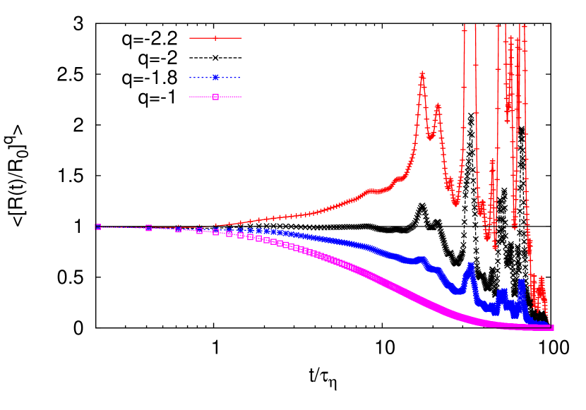
Figure 2: Time evolution of different moments of relative separation $R(t)$ as a function of time in the 2D simulations ($R_{0}=1.1\eta$). Different point styles represent $q=-1.0$, $q=-1.8$, $q=-2.0$ and $q=-2.2$ (from bottom to top).

The exponential time dependence of $\left<R^{q}(t)\right>$ observed in Fig. 2 is expected to be a long time feature of any linear flow with temporal correlations decaying fast enough Falkovich et al. (2001), Balkovsky and Fouxon (1999). Specifically, $E(q,t)\equiv\ln\left<\left(R(t)/R_{0}\right)^{q}\right>$, the cumulant generating function of $\beta=\ln\left(R(t)/R_{0}\right)$, should take at long times the form $E(q,t)=L(q)t$. We remark that the finite-time Lyapunov exponent $\sigma=\beta/t$ tends to the Lagrangian Lyapunov exponent, $\lambda$, in the long time limit Cencini et al. (2010).

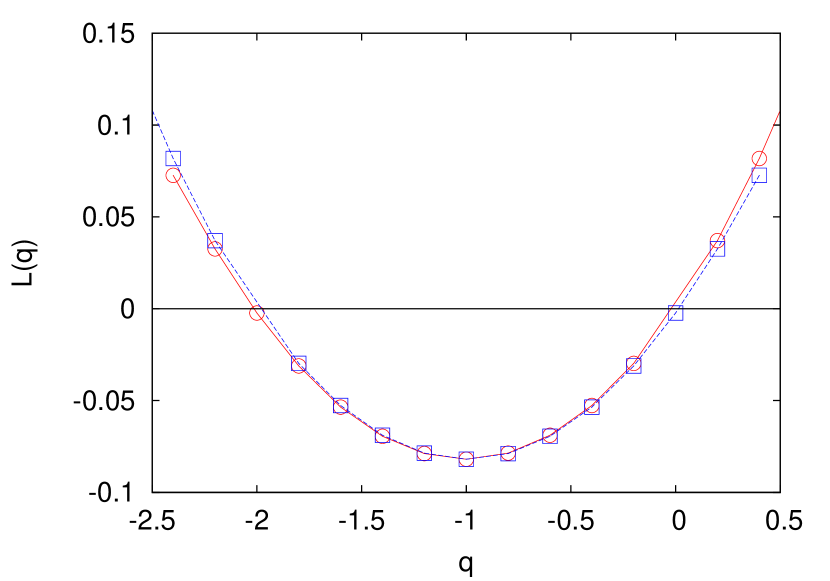
Figure 3: $L(q)$ obtained from fitting $\left<R(t)^{q}\right>$ with $R_{0}^{q}e^{L(q)t}$ in the time interval $2\leq t/\tau_{\eta}\leq 10$ for the 2D simulations ($R_{0}=1.1\eta$). In order to show the symmetry with respect to $q=-1$, both $L(q)$ (red circles) and $L(-2-q)$ (blue squares) are plotted.

We obtain $L(q)$ shown in Fig. 3 by fitting $\left<R(t)^{q}\right>=R_{0}^{q}e^{L(q)t}$ for times $0.4\leq\lambda t\leq 2$. Evidently $L(q)$ is perfectly symmetric with respect to $q=-d/2=-1$, i.e $L(q)=L(-q-2)$, implying in particular that $L(-2)=0$ as expected. This symmetry can be extended to the symmetry $E(q,t)=E(-q-2,t)$ holding at any time $t$, as we demonstrate in the bottom figure of Fig. 5 for $t=0.2\tau_{\eta}$. This is a general property of a two-dimensional linear incompressible and isotropic flow. In fact, this follows from the relation

$$\int\left(\frac{R(t)}{R_{0}}\right)^{q}d\Omega_{0}=\int\left(\frac{R(t)}{R_{0}}\right)^{-q-2}d\Omega_{0}$$ (3)

which, as we will show, holds for every velocity realization. Indeed, using the definition of $E(q)$ one obtains $E(q,t)=E(-q-2,t)$ for an isotropic flow by taking the average of (3) over velocity realizations, conditioned that the averages exist.

To demonstrate (3) we recall that for a linear flow with a given velocity realization the following decomposition can be used

$$\frac{R(t)^{2}}{R_{0}^{2}}=\hat{R}_{0}^{T}O^{T}(t)\Lambda(t)O(t)\hat{R}_{0}$$ (4)

where $O(t)$ is an orthogonal matrix and $\Lambda$ a diagonal matrix with entries $e^{\rho_{1}(t)}$ and $e^{\rho_{2}(t)}$ Cardy et al. (2008)Falkovich et al. (2001). For an incompressible flow $\det\Lambda=1$ so that in 2D $\rho_{1}=-\rho_{2}\equiv\rho$. Using (4) the integration over $\hat{R}_{0}$ can be written as

$$\begin{split}\int\left(\frac{R(t)}{R_{0}}\right)^{q}d\Omega_{0}=\int_{0}^{2\pi}\left[\hat{e}^{T}(\theta)\Lambda(t)\hat{e}(\theta)\right]^{q/2}d\theta\end{split}$$ (5)

where $\hat{e}=(\cos(\theta),\sin(\theta))$ and a change of integration variable absorbed the additional rotation $O(t)$ in (4). On the other hand, (1) implies

$$\int\left(\frac{R(t)}{R_{0}}\right)^{q}d\Omega_{0}=\int\left(\frac{R_{0}}{R(t)}\right)^{-q-2}d\Omega_{t}$$ (6)

and $R_{0}/R(t)$ can be decomposed, similarly to (4), using the flow backward in time

$$\frac{R_{0}^{2}}{R(t)^{2}}=\hat{R}_{t}^{T}O^{T}(-t)\Lambda(-t)O(-t)\hat{R}_{t}.$$ (7)

The inversion of the linear transformation between $\textbf{R}(t)$ and $\textbf{R}(0)$ implies $\Lambda(-t)=\Lambda^{-1}(t)$ Cardy et al. (2008). Then, $\Lambda^{-1}(t)$ is related to $\Lambda(t)$ by conjugation with a rotation matrix since $\Lambda=diag(e^{\rho},e^{-\rho})$. This property is actually a consequence of the symplectic structure of a 2D incompressible flow- for a symplectic flow the eigenvalues of $\Lambda$ come in pairs of the form $e^{\pm\rho_{i}}$ Cencini et al. (2010). Therefore for any $m$, shifting the integration variable similarly to (5),

$$\begin{split}\int\left(\frac{R_{0}}{R(t)}\right)^{m}d\Omega_{t}=\int_{0}^{2\pi}\left[\hat{e}^{T}(\theta)\Lambda(t)\hat{e}(\theta)\right]^{m/2}d\theta\end{split}$$

which by comparison to (5) leads to

$$\begin{split}\int\left(\frac{R_{0}}{R(t)}\right)^{m}d\Omega_{t}=\int\left(\frac{R_{0}}{R(t)}\right)^{-m}d\Omega_{0}.\end{split}$$ (8)

Finally, combining equation (8) with $m=-q-2$ together with equation (6) yields (3).

The symmetry of $E(q)$ implies a symmetry of the probability density function (pdf) $P\left(\beta(t)\right)$, $\beta=\ln\left(R(t)/R_{0}\right)$, which can be obtained by first extending the symmetry of $E(q)$ to complex $q$ and then retrieving the pdf by an inverse Laplace transform of $\exp[E(q)]$. Using the symmetry and a change of variables in the integration, one gets for any time $t$

$$\frac{P(\beta(t)=y)}{P(\beta(t)=-y)}=e^{2y}=J(y)$$ (9)

where $J(\ln\left(R(t)/R_{0}\right))$ is the Jacobian of the transformation (1) from time zero to time $t$, in 2D.

Figure 4: Verification of the symmetry relation (9), $\beta=\ln\left(R(t)/R_{0}\right)$, in the 2D simulations. The solid straight line corresponds to the analytical prediction.

In the asymptotically long-time limit (9), which is numerically verified in Fig. 4, turns into an Evans-Cohen-Morriss Evans et al. (1993) or Gallavotti-Cohen Gallavotti and Cohen (1995) type fluctuation relation. Indeed, the function $L(q)$ is the Legendre transform of the long-time large deviation function $G(\sigma)$ so that the symmetry in $L(q)$ implies:

$$G(-\sigma)=G(\sigma)+2\sigma$$ (10)

which can also be deduced directly from (9). This relation resembles the Evans-Cohen-Morriss-Gallavotti-Cohen relation, and even more so the relation found in Chetrite et al. (2007), but is different from them. Note that we do not assume a time reversible velocity ensemble and work with an incompressible flow (implying zero entropy production in the context of dynamical systems). The two dimensionality of the flow plays a crucial role in the derivation.

In Fig. 5 we show $E(q,t)$ for short times, $t\leq 8\tau_{\eta}$ as a function of $q$, comparing two distinct initial separations. For $R_{0}=1.1\eta$ all curves cross zero at $q=-2$, up to time $t=8\tau_{\eta}$, while for $R_{0}=50\eta$, which is at the border of the linear scaling range, the initial crossing is shifted above $-2$, and the intersection point changes with time (see middle Figure). The appearance of the initial crossing above $-2$ in the latter can be explained using a Taylor expansion of $\left<\left(R(t)/R_{0}\right)^{q}\right>$ around $t=0$, see equations (11),(15) and (14) in the analysis of the experimental results, as well as Falkovich and Frishman (2013).

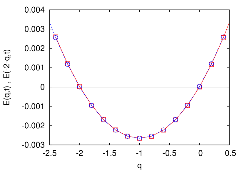
Figure 5: $\ln\left<\left(R(t)/R_{0}\right)^{q}\right>$ as a function of $q$ for two different initial separations $R_{0}=1.1\eta$ (upper plot) and $R_{0}=50\eta$ (middle plot). Different curves represent different times. Lower plot: $E(q,t)$ (red circles) and $E(-2-q,t)$ (blue squares) for $t=0.2\tau_{\eta}$ and $R_{0}=1.1\eta$. Data from 2D simulations.

Conservation in 3D - DNS results

Lagrangian tracers are introduced into a numerical simulation of three-dimensional turbulence in a cubic box at $Re_{\lambda}=107$. The tracers are placed in the flow when it has reached a steady state and their trajectories are numerically integrated. Turbulence is generated by a large scale, $\delta$-correlated random forcing. Small scales are well resolved in the simulation (for which $k_{max}\eta=1.3$). More than 130000 pairs were integrated for times up to about 10 $\tau_{\eta}$ for 300 realizations each, while more than 30000 pairs were integrated for 150 realizations for longer times. The two datasets are overlapping for shorter times so that consistency of the statistics could be checked.

In Fig. 6 we show the second order longitudinal velocity structure function. Up to separations of about $7\eta$ the scaling exponent of $\left<u_{l}^{2}(R)\right>$ is close to $2$, although deviations are also observed earlier.

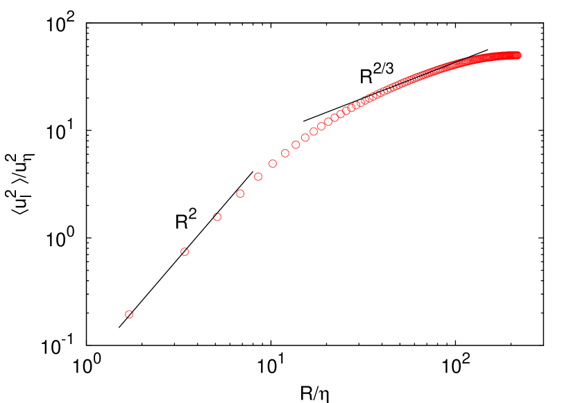
Figure 6: Second order longitudinal velocity structure function for the 3D numerical simulation. The two lines represent the smooth $R^{2}$ and rough $R^{2/3}$ behaviors.

In Fig. 7, $\ln\left<\left(R(t)/R_{0}\right)^{q}\right>$ as a function of $q$ is presented for three different initial separations and for various times. A clear crossing of zero at $q=-3$ can be observed up to time $t=8\tau_{\eta}$ for $R_{0}=1.7\eta$. For $R_{0}=6.7\eta$, which lies at the transition from the dissipative range, the initial crossing is shifted above $-3$ (see intermediate Figure) a trend which is much more pronounced for $R_{0}=70\eta$ at the inertial range. This is the same trend that appeared in the 2D simulation and can be explained in a similar way. Evidently, this shifted crossing point cannot also correspond to a conservation law, as it is time dependent, for both separations.

Figure 7: $\ln\left<\left(R(t)/R_{0}\right)^{q}\right>$ as a function of $q$ for different initial separations $R_{0}=1.7\eta$ (upper plot), $R_{0}=6.76\eta$ (middle plot), $R_{0}=70\eta$ (lower plot). The different curves represent different times. Data from 3D simulations.

Although theoretically $\left<\left(R(t)/R_{0}\right)^{-3}\right>$ is an all time conservation law, in reality after some time pairs reach separations where a linear flow approximation no longer works, see also Fig. 2 and its discussion for the 2D flow. We study the exit from the conservation regime of $\left<\left(R(t)/R_{0}\right)^{-3}\right>$ for $R_{0}=1.7\eta$ in Fig. 8. After $t\sim 8-10\tau_{\eta}$ wild fluctuations, as well as a decrease in value, appear for $\left<\left(R(t)/R_{0}\right)^{q}\right>$ with $q<-2$. This behaviour can be explained by the formation of a power-law dependence on separation in the separations pdf at small $R$, see Fig. 9, together with a shift of the average separation to larger values. Such a dependence has been shown to develop for initial separations both in the inertial range and in the dissipative one in Bitane et al. (2013). In Fig. 9(a) $P(R/R_{0})$ is shown for different times for the 3D simulations. Indeed the left tail shows a power law dependence $R^{\alpha}$, with $\alpha$ decreasing until reaching $\alpha\sim 2$ at times $10\lesssim t/\tau\lesssim 20$. This explains why the moment $\langle R^{-3}\rangle$ starts diverging somewhere in this interval. For larger times we observe a further decrease in $\alpha$ (not shown), compatible with the values observed in Bitane et al. (2013). This power law behaviour may be due to the contribution of trajectories which left the viscous subrange and returned to $R<R_{0}$. Indeed, $P(R/R_{0})$ is expected (at long enough times) to have a log-normal shape near its maximum, as long as the separation remains in the viscous range Falkovich et al. (2001). In our 3D simulations, $P(R/R_{0})$ never displays a log-normal shape, probably as a consequence of the limited extension of the viscous range. On the contrary, the PDF’s of separations are clearly log-normal in the 2D case Fig. 9(b). Although the statistics are not sufficient to distinguish the development of a power-law dependence in the left tail in the 2D data, the large fluctuations in Fig. 2 point towards a behaviour analogous to the 3D case.

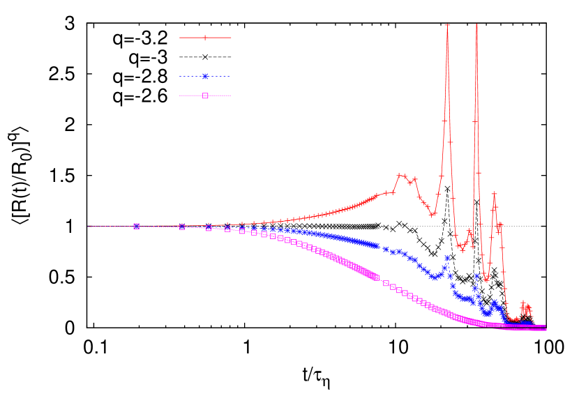
Figure 8: $\left<\left(R(t)/R_{0}\right)^{q}\right>$ as a function of time for various $q$, the initial separation is $R_{0}=1.7\eta$. Different symbols represent $q=-2.6$, $q=-2.8$, $q=-3.0$ and $q=-3.2$ (from bottom to top). Data from 3D simulations.

Figure 9: $P(R(t)/R_{0})$ for the smallest available initial separations in the 3D (a) and the 2D simulations (b) respectively. While the 3D case shows the development of power-law tails for small separations, in the 2D case all PDFs are close to log-normal curves, marked by solid lines in (b)

.

Conservation in 3D - experimental results

In the previous sections we have presented supporting evidence from numerical simulations, both in two and three dimensions, for the conservation of $\left<R^{-d}\right>$ for an isotropic flow at small enough scales. It is interesting to check if similar results can be obtained from laboratory experimental data where the access to very small initial separation is limited by both physical and statistical constraints. It is to this end that we turn to data from the experimental set up described in Liberzon et al. (2012), where neutrally buoyant particles are tracked inside a water tank of dimensions $32\times 32\times 50cm^{3}$. The turbulent flow, with $Re_{\lambda}=84$ for our data set, is generated by eight propellers at the tanks corners and particles are tracked in space and time using four CCD cameras. The cameras are focused on a small volume of $1cm^{3}$ to resolve the smallest scales (the Kolmogorov scale is $\eta=0.4mm$). At such small scales, the flow is expected to be isotropic. We study pairs of particles with initial separations of a few $\eta$, for which numerical and previous experimental studies of turbulent flows found an approximately linear flow Watanabe and Gotoh (2007); Bewley et al. (2013); Zhou and Antonia (2000); Benzi et al. (1995); Ishihara et al. (2009); Lohse and Müller-Groeling (1995).

As isotropy and a linear dependence of velocity differences on separation are the two assumptions entering the prediction of the conservation of $\left<R^{-3}\right>$, the experimental set up described above appears to be appropriate to test it. Unfortunately, a direct check of these assumptions does not seem to support their applicability.

Figure 10: Second order velocity structure function in the 3D experiment as deduced from the initial relative velocity of pairs of particles with initial separation $R_{0}$, normalized with the squared Kolmogorov velocity $u^{2}_{\eta}$. Inset: The local slope $d\ln\left<\textbf{u}^{2}\right>/d\ln R_{0}$ as a function of the separation. The dashed line represents the scaling $\left<\textbf{u}^{2}\right>\propto R_{0}^{1.5}$.

In Fig.  10 we present $\left<\textbf{u}^{2}\right>$, using the relative velocity of particles with separation $R_{0}$. Here and in the following $\left<\right>$ denotes an average over pairs in an ensemble with a given initial separation. When it is applied to functions of the relative velocity or acceleration at a given scale it denotes the average over the pairs with the corresponding initial separation, taken at $t=0$. As can be seen from the inset of Fig. 10, if any scaling regime, $\left<\textbf{u}^{2}\right>\propto R_{0}^{\zeta_{2}}$, is to be assigned, it would be with scaling exponent $\zeta_{2}=1.5$ rather than $\zeta_{2}=2$. It seems that in order to access the linear flow regime in this system even smaller distances should be probed, which is not experimentally accessible at the moment.

For separations at the transition between inertial and dissipative ranges, as those apparently probed in this experiment, there is currently no theoretical prediction regarding the existence of a conservation law. Still, in the spirit of the conservation law in the dissipative range, we can look for $q$ such that $\left<\left(R(t)/R_{0}\right)^{q}\right>=1$. Notice that as a function of $q$, $\left<\left(R(t)/R_{0}\right)^{q}\right>$ is convex and at each time $t$ it crosses $1$ at $q=0$ and either has one more crossing point, denoted by $q^{*}(t)$, or none. It would be possible to establish the existence of a conservation law, with $q=q^{*}$, if $q^{*}$ exists and is time independent. To get an idea of what value $q^{*}$ can take we use the Taylor expansion of $\left<R^{q}(t)\right>$ around $t=0$ (no assumption is made about the nature of the flow):

$$\left<\left(\frac{R(t)}{R_{0}}\right)^{q}\right>=1+\frac{\left<u_{l}^{2}\right>}{R_{0}^{2}}\frac{qt^{2}}{2}\left[q-q_{e}(t)\right]+O(t^{3})$$ (11)

with

$$q_{e}(t)\equiv c-\frac{2\left<u_{l}\right>R_{0}}{t\left<u_{l}^{2}\right>}; c\equiv 2-\frac{\left<\textbf{u}^{2}\right>+\left<a_{l}\right>R_{0}}{\left<u_{l}^{2}\right>}$$ (12)

where $u_{l}=\textbf{u}\cdot\hat{R}_{0}$, $a_{l}=\textbf{a}\cdot\hat{R}_{0}$ and a is the relative acceleration. This implies that the conservation law described above can exist only if $q_{e}(t)$ is time independent, so that $q^{*}=q_{e}=c$. This is of course only a necessary but not a sufficient condition.

The time dependence of $q_{e}$ comes from the first order in the Taylor expansion $\propto\left<u_{l}\right>$. It, as well as $\left<a_{l}\right>$, should be zero for a statistically homogeneous or a statistically isotropic flow. Obviously in an experiment $\left<u_{l}\right>$ can never be exactly zero, but it can be small enough so that at the shortest times measured the time dependent term in $q_{e}$ would be negligible compared to the time independent part, $c$ in (12).

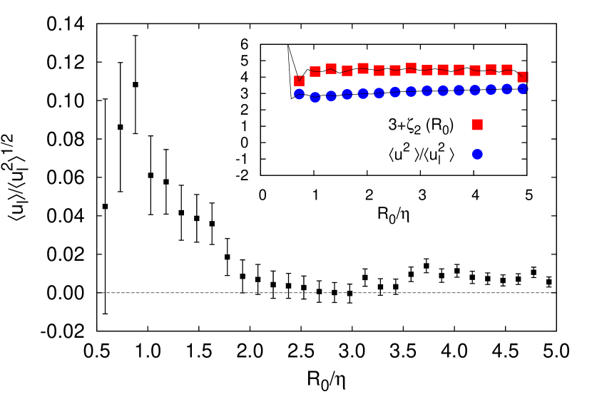
Figure 11: Average longitudinal relative velocity as a function of initial separation for pairs of particles at $t=0$. The velocity is normalized by the initial rms longitudinal relative velocity. Inset: The LHS and the RHS of equation (14) are displayed as a function of $R_{0}$.

In the inset of Fig. 11 we present $\left<u_{l}\right>$ normalised by the rms relative velocity. The strong bias towards positive $\left<u_{l}\right>$ for $R_{0}<2\eta$ is probably the result of the filtration of pairs with life times smaller than $0.5\tau_{\eta}$. Indeed, pairs with approaching particles at small separations are harder to track and are therefore frequently short lived as well as more prone to errors. A similar problem might also be the cause of the positive bias for $R_{0}\gtrsim 3\eta$, where particles with a large relative velocity are more common. Then, particles approaching each other with a large speed reach small scales quickly and are lost more easily. When the restriction on the life time of the pairs is lifted a negative bias emerges. It therefore appears that using $\left<u_{l}\right>$ for pairs of particles to determine the isotropy or homogeneity of the flow is problematic. For our purposes, note that for an observation of the conservation of $\left<R^{c}(t)\right>$ to be possible the value of $\left<u_{l}\right>$ must be as small as possible. Initial separations $R_{0}=2.6\eta-3\eta$ seem most appropriate.

For a d-dimensional incompressible flow that is statistically isotropic a simpler formula for $q_{e}$ can be written. For such a flow (see also Van De Water and Herweijer (1999))

$$\left\langle\textbf{u}^{2}\right>-\left\langle u_{l}^{2}\right>=\frac{1}{R_{0}}\frac{d}{dR_{0}}\left(R_{0}^{2}\left\langle u_{l}^{2}\right>\right).$$ (13)

which can be used to write

$$\frac{\left\langle\textbf{u}^{2}\right>}{\left<u_{l}^{2}\right>}=(d+\zeta_{2}(R_{0})); \zeta_{2}(R_{0})=\frac{d\ln\left<u_{l}^{2}\right>}{d\ln R_{0}}$$ (14)

implying that in (12)

$$q_{e}=c=2-d-\zeta_{2}(R_{0})=-1-\zeta_{2}(R_{0}).$$ (15)

As a side note, we remark that if $\zeta_{2}$ is constant, like in the inertial range, the initially slowest changing function, $R(t)^{c}=R(t)^{2-d-\zeta_{2}}$, is independent of $R_{0}$ Falkovich and Frishman (2013). More generally, requiring only $\left<u_{l}\right>=0$, the $R_{0}$ independent slowest varying (among twice differentiable functions of $R$) function $F(R)$, is determined by demanding $\left<d^{2}F(R)/dt^{2}\right>=0$, resulting in

$$F(R)\propto\int_{a}^{R}\exp\left[\int_{a}^{x}\frac{-\left\langle u_{T}^{2}\right>}{z\left\langle u_{l}^{2}\right>}dz\right]dx.$$ (16)

with $a$ an arbitrary separation and $u_{T}^{2}=\textbf{u}^{2}-u_{l}^{2}$. For a 3-dimensional isotropic flow this formula reduces with the help of (13) to

$$F(R)\propto\int_{a}^{R}\frac{1}{x^{2}\left\langle u_{l}^{2}\right>}dx.$$ (17)

Here, however, we focus on the simpler functions $F(R)=R^{q_{e}}$, which, through $q_{e}$, are $R_{0}$ dependent.

The isotropy assumption is checked using equation (14), as suggested in Van De Water and Herweijer (1999), in the inset of Fig. 11 where we present both the LHS of this equation and its RHS as a function of initial separation. The difference between the two is about $1.5$ for most separations, implying that isotropy is violated. It could also be that the flow is, in fact, isotropic: although in theory measuring relative velocities for pairs of particles at a given distance is the same as using two fixed probes in the flow, in practice it might not be so (for example due to correlations entering through the method of pair selection).

Figure 12: The exponent $q^{*}(t)$, deduced by matching $\left<R(t)^{q^{*}}\right>=R_{0}^{q^{*}}$, plotted as a function of $R_{0}$ at different times. The dashed line represent the prediction $q^{*}(t)=c$, with $c$ from (12). Inset: The negative of the contribution to $c$ due to $\left<a_{l}\right>$, $R_{0}\left<a_{l}\right>/\left<u_{l}^{2}\right>$, plotted as a function of $R_{0}$.

In any case, we conclude that the prediction (15) should not work for our data, as indeed it does not, and instead use in the following the more general definition of $c$, (12). In Fig. 12 we present the exponent $q^{*}(t)$, as deduced from the data, for five consecutive times and compare it to $c$. As expected, $q^{*}(t)$ appears approximately constant and equal to $c$ for the separations where $\left<u_{l}\right>$ is smallest. Note that $c$ has a non-negligible contribution coming from the deviation of $\left<a_{l}\right>$ from zero. This contribution is displayed in the inset of Fig. 12.

Figure 13: The evolution in time of $\left<\left(R(t)/R_{0}\right)^{q}\right>$ for pairs with initial separation of $R_{0}=2.6\eta$. The dashed dotted curve represents $q=c=-1.32$

We are now in a position to ask if for the separation where initially $q^{*}(t)\approx c$, $\left<R^{c}(t)\right>$ is just a slowly varying function or a true conservation law. In Fig. 13, for the separation $R_{0}=2.6\eta$, we compare $\left<\left(R(t)/R_{0}\right)^{q}\right>$ as a function of time for different $q$s, including $q=c$. After a time shorter than $\tau_{\eta}$, $\left<R^{c}(t)\right>$ noticeably decreases. During this time the average separation between particles in a pair changes by less than one percent. It is thus improbable that $\left<R^{c}(t)\right>$ is truly constant up to that time, but rather that it changes slowly, meaning it is not a conserved quantity. We conclude that, at the scales accessible to this experiment, a power-law-type of conservation law probably does not exist but a slowly varying function of the separation can be identified.

Acknowledgements A.F is grateful to G. Falkovich and E. Afik for many useful discussions and comments. She would also like to thank J. Jucha for her valuable input on the experimental data and O. Hirschberg for recognizing the fluctuation relations. A.F is supported by the Adams Fellowship Program of the Israel Academy of Sciences and Humanities.

References

- Falkovich and Frishman (2013) G. Falkovich and A. Frishman, Phys. Rev. Lett. 110, 214502 (2013).
- Falkovich et al. (2001) G. Falkovich, K. Gawȩdzki, and M. Vergassola, Rev. Mod. Phys. 73, 913 (2001).
- Celani and Vergassola (2001) a. Celani and M. Vergassola, Phys. Rev. Lett. 86, 424 (2001).
- Falkovich (2014) G. Falkovich, Journal of Plasma Physics FirstView, 1 (2014).
- Zel’Dovich et al. (1984) Y. B. Zel’Dovich, A. A. Ruzmaikin, S. A. Molchanov, and D. D. Sokoloff, Journal of Fluid Mechanics 144, 1 (1984).
- Jarzynski (1997) C. Jarzynski, Phys. Rev. Lett. 78, 2690 (1997).
- Chetrite and Gawȩdzki (2008) R. Chetrite and K. Gawȩdzki, Communications in Mathematical Physics 282, 469 (2008).
- Evans et al. (1993) D. Evans, E. Cohen, and G. Morriss, Phys. Rev. Lett. 71, 2401 (1993).
- Gallavotti and Cohen (1995) G. Gallavotti and E. Cohen, Phys. Rev. Lett. 74, 2694 (1995).
- Boffetta et al. (2002) G. Boffetta, a. Celani, S. Musacchio, and M. Vergassola, Phys. Rev. E 66, 026304 (2002).
- Bernard (2000) D. Bernard, Europhys. Lett. 50, 333 (2000).
- Boffetta and Ecke (2012) G. Boffetta and R. E. Ecke, Annu. Rev. Fluid Mech. 44, 427 (2012).
- Balkovsky and Fouxon (1999) E. Balkovsky and A. Fouxon, Phys. Rev. E 60, 4164 (1999).
- Cencini et al. (2010) M. Cencini, F. Cecconi, and A. Vulpiani, Chaos: From Simple Models to Complex Systems, Series on advances in statistical mechanics (World Scientific, 2010).
- Cardy et al. (2008) J. Cardy, G. Falkovich, K. Gawȩdzki, S. Nazarenko, and O. Zaboronski, Non-equilibrium Statistical Mechanics and Turbulence, London Mathematical Society Lecture Note Series (Cambridge University Press, 2008).
- Chetrite et al. (2007) R. Chetrite, J.-Y. Delannoy, and K. Gawedzki, J. Stat. Phys. 126, 1165 (2007).
- Bitane et al. (2013) R. Bitane, H. Homann, and J. Bec, J. Turbul. 14, 23 (2013).
- Liberzon et al. (2012) A. Liberzon, B. Lüthi, M. Holzner, S. Ott, J. Berg, and J. Mann, Physica D: Nonlinear Phenomena 241, 208 (2012), special Issue on Small Scale Turbulence.
- Watanabe and Gotoh (2007) T. Watanabe and T. Gotoh, J. Fluid Mech. 590, 117 (2007).
- Bewley et al. (2013) G. P. Bewley, E.-W. Saw, and E. Bodenschatz, New J. Phys. 15, 083051 (2013).
- Zhou and Antonia (2000) T. Zhou and R. a. Antonia, J. Fluid Mech. 406, 81 (2000).
- Benzi et al. (1995) R. Benzi, S. Ciliberto, C. Baudet, and G. R. Chavarria, Physica D: Nonlinear Phenomena 80, 385 (1995).
- Ishihara et al. (2009) T. Ishihara, T. Gotoh, and Y. Kaneda, Annu. Rev. Fluid Mech. 41, 165 (2009).
- Lohse and Müller-Groeling (1995) D. Lohse and A. Müller-Groeling, Phys. Rev. Lett. 74, 1747 (1995).
- Afik and Steinberg (2015) E. Afik and V. Steinberg, ArXiv e-prints (2015), submitted, arXiv:1310.1371 [nlin.CD] .
- Van De Water and Herweijer (1999) W. Van De Water and J. a. Herweijer, J. Fluid Mech. 387, 3 (1999).