Heterophase liquid states: Thermodynamics, structure, dynamics

Abstract

An overview of theoretical results and experimental data on the thermodynamics, structure and dynamics of the heterophase glass-forming liquids is presented. The theoretical approach is based on the mesoscopic heterophase fluctuations model (HPFM) developed within the framework of the bounded partition function approach. The Fischer cluster phenomenon, glass transition, liquid-liquid transformations, parametric phase diagram, cooperative dynamics and fragility of the glass-forming liquids is considered.

Key words: glass-forming liquids, glass transition, Fischer’s cluster, polymorphism, parametric phase diagram

PACS: 78.35.+c, 64.70.Pf

Abstract

Представлено огляд теоретичних результатiв та експериментальних даних щодо термодинамiки, структури i динамiки гетерофазних склоутворювальних рiдин. Теоретичний пiдхiд базується на моделi мезоскопiчних гетерофазних флуктуацiй, яка була розвинута в рамках пiдходу обмеженої статистичної функцiї. Розглянуто явище кластер Фiшера, перехiд у фазу скла, перетворення рiдина-рiдина, параметричну фазову дiаграму, колективну динамiку i фрагiльнiсть склоутворювальних рiдин.

Ключовi слова: склоутворювальнi рiдини, перехiд у фазу скла, кластер Фiшера, полiморфiзм, параметрична фазова дiаграма

1 Introduction

Structure of a glass-forming liquid and glass possesses a short-range and medium-range order (SRO and MRO) rather than a long-range order (LRO). Below the crystallization temperature, $T_{m}$, precautions have to be taken to avoid crystallization or a quasi-crystalline structure formation and to prevent the supercooled liquid state down to the glass transition. Therefore, a liquid can be transformed into amorphous (glassy) solid only if cooling is fast enough to avoid crystallization. As a result, the liquid is non-equilibrium and unstable at the glass transition. For this reason a description of the glass transition cannot be based on the canonic Gibbs statistics. A palliative approach based on the bounded statistics can be formulated as follows.

If the cooling time is much longer than the equilibration time of the liquid structure on scale $\xi$ [let us denote this time by $\tau\left(\xi\right)$] and no significant structural correlation occurs on scales $r>\xi$, one can consider the glass transition as a sequence of transformations of the structure states which are equilibrated just on the scales $r<\xi$. Statistical description of such a liquid can be developed if we exclude from the statistics the states with the correlation scale $r>\xi$ and, on the other hand, ensure that the observation time, $\tau_{\textrm{obs}}$, is much longer than $\tau\left(\xi\right)$. In this case, the Gibbs partition function can be replaced by the bounded partition function which is used then to determine the free energy of the partially equilibrated liquid. Limitation of the phase space due to the exclusion of the states with correlation lengths $r>\xi$ leads to an increase of the free energy of the equilibrium state. The standard Gibbs statistics restores with $\xi\to\infty$. The observation time limits from above the scale of the relaxation time $\tau\left(\xi\right)$ and, consequently, the scale $\xi$, because $\tau\left(\xi\right)$ increases $\sim\xi^{\theta}$ (the exponent $\theta$ depends on the features of the relaxation kinetics).

The spatial scale of the SRO, $\xi_{\textrm{SRO}}$, is minimal among the possible correlation lengths in the liquid. Accordingly, $\tau\left(\xi_{\textrm{SRO}}\right)$ is the shortest structure relaxation time because it is controlled by rearrangement of a comparatively small number of directly interacting molecules. The formation of longer correlations, with $\xi\gg\xi_{\textrm{SRO}}$, which involves a large number of molecules in rearrangement and is driven by relatively weak multi-molecular forces, takes much longer than $\tau\left(\xi_{\textrm{SRO}}\right)$ time. The liquid or glass, which is equilibrated on the scale $r\sim\xi_{\textrm{SRO}}$ without considerable correlations on larger scales, is the minimally ordered amorphous state which can be considered using the bounded statistics method. For this reason, as the first step, the bounded partition function should be considered taking into account the states with equilibrated SRO.

It is experimentally established that the glass-forming liquids are heterophase (their structure consists of the mutually transforming fluid-like and solid-like substructures). Observations of the heterophase structure of glass-forming liquids are numerous. Among significant observations of the last decades we should mention the formation of the Fischer cluster (fractal aggregate of the solid-like HPF in glass-forming organic liquids and polymers [1, 2, 3, 4, 5, 6, 7, 8, 9, 10]), evolutive HPF in supercooled triphenyl phosphit observed in [11], and others.

Many types of the SRO usually coexist in glasses. In Bernal’s mechanical model of the dense random packing of hard spheres, six types of the local order (Bernal’s holes) are statistically significant and nearly one third of them are non-crystalline [13]. Similar results are obtained using computer simulations of liquids and glasses with different interatomic potentials [14, 15, 16, 17, 18].

A wide spectrum of relaxation times in glass-forming liquids is observed due to the variety of SRO types (see [19, 20] and references cited).

Since SRO is the molecular order formed due to microscopic forces, the correlation length $\xi_{\textrm{SRO}}$ is equal to or exceeds the range of direct molecular interactions. Therefore, to describe heterophase states, a mesoscopic theory is needed, in which molecular species of size $r\sim\xi_{\textrm{SRO}}$ specified by SRO are ‘‘elementary’’ structural elements rather than molecules. These are not molecular potentials that determine the equilibrium states and relaxation dynamics of heterophase states but rather the parameters of heterophase fluctuation interactions connected with molecular potentials. Evidently, the mesoscopic Hamiltonian is more universal but less detailed than the microscopic Hamiltonian specified by molecular potentials. Parameters of the mesoscopic Hamiltonian can be considered as phenomenological coefficients with averaged out microscopic details of molecular interaction.

These ideas are in the base of the heterophase fluctuation model (HPFM) [10, 21, 22, 23, 24, 25, 26, 27] which is considered in sections 2–6 and in appendixes A and B. It is further used while considering the issues of the thermodynamics of a liquid-glass transition and polymorphous transformations of glass-forming liquids and glasses induced by the SRO reordering and mutual ordering of heterophase fluctuations (section 7 and appendix C). The cooperative relaxation dynamics of a heterophase liquid is considered within the framework of phenomenological model formulated in HPFM [10, 22] (section 8). Conclusive remarks are placed in section 9.

2 Hetrophase fluctuations and the order parameter

The heterophase fluctuation is an embryo of a foreign phase in the matrix phase. In many liquids, even in normal state (above the crystallization temperature, $T_{m}$), solid-like species are revealed by means of difractometry. The first observation of such heterophase fluctuations (HPF) was made by Stewart and Morrow [28]. They have discovered sybotactic groups (transient molecular solid-like clusters possessing specific short-range order) in simple alcohols above $T_{m}$.

The HPF are non-perturbative fluctuations in contrast to perturbative fluctuations of physical quantities near their equilibrium values in the homophase state. Theory of the heterophase states originates from Frenkel’s paper [29]. Frenkel has coined the term ‘‘heterophase fluctuations’’ and explored the thermodynamics of heterophase states of fluid and gas in the vicinity of the phase coexistence curve. Frenkel’s theory is applicable to all kinds of the coexisting phases (including the fluid and solid phases) far below the critical point. In this case, the amount of substance belonging to HPF is small, and thus Frenkel’s droplet model, with non-interacting nuclei of a foreign phase, properly describes the heterophase state.

Frenkel’s theory fails in the case of strong HPF, when the fraction of molecules belonging to the ‘‘droplets’’ is large (for example, when it is near or exceeds the percolation threshold), and thus droplet-droplet interaction cannot be neglected. Besides, this theory was not generalized to include in its consideration the states with many SRO-types of the nucleating ‘‘droplets’’. Both these restrictions of the Frenkel model are obviated in the HPFM.

The HPFM is based on the statistics of the transient solid-like and fluid-like mesoscopic species (clusters) which are called $s$-fluctuons and $f$-fluctuons, respectively. By definition, each fluctuon is specified by SRO. The minimal size of a fluctuon is equal to the SRO correlation length, $\xi_{\textrm{SRO}}$. An arbitrary number of types of the $s$-fluctuons, $m\geqslant 1$, can be included into consideration.

To escape needless complications, let us assume that the fluctuons are uniform-sized with size $r_{0}$ and with the number of molecules per fluctuon equal to $k_{0}\sim r_{0}^{3}$. Thus, $\xi_{\textrm{SRO}}\simeq r_{0}$. This simplification is reasonable from the physical point of view because in the both states SRO is formed due to the action of the same microscopic forces, and the difference of the densities of a liquid and a solid usually amounts to just a few percent. The solid-like and fluid-like fractions consist of $s$- and $f$-fluctuons, respectively.

Let us denote by $N$ the total number of molecules of liquid and by$N_{f},N_{1},\ldots,N_{m}$ the numbers of molecules belonging to $f$- and $s$-fluctuons,

$$N_{f}+N_{1}+\ldots+N_{m}=N.$$ (2.1)

The total number of fluctuons is $N_{\textrm{fluct}}=N/k_{0}$.

The $(m+1)$-component order parameter of the heterophase liquid is determined as follows:

$$\left\{c\right\}=(c_{f},c_{1},\ldots,c_{m}),\qquad c_{i}=\frac{N_{i}}{N}\geqslant 0,\qquad i=f,1,\ldots,m\,,$$ (2.2)

$$c_{f}+c_{1}+\ldots+c_{m}\equiv c_{f}+c_{s}=1.$$ (2.3)

Evidently, $c_{i}$ is the probability of the molecule belonging to $i$-th type of fluctuons. $N_{s}=N_{1}+N_{2}+\ldots+N_{m}=c_{s}N$ is the number of molecules of the solid-like fraction. The spatial distribution of the fluctuons on scale $r\gg r_{0}$ can be described by the order parameter fields $c_{i}(x)$ with mean values equal to $c_{i}$.

Let us regard the $k$-th type $s$-fluctuons as statistically insignificant if $c_{k}\ll m^{-1}$. The $f$-fluctuons become statistically insignificant if $c_{f}\ll 1$. The exclusion of the statistically insignificant components of the order parameter from consideration allows one to simplify the equations of HPFM. The statistically insignificant entities, when necessary, can be included into consideration as perturbations.

3 The quasi-equilibrium glass transition and ‘‘ideal’’ glass

Let us consider more in detail the formulated in Introduction conditions under which the glass transition with equilibrated SRO takes place:

1. The liquid cooling time or the observation time, $\tau_{\textrm{obs}}$, should be less than the time of crystallization,

   $$\tau_{\textrm{obs}}\ll\tau_{\textrm{LRO}}\,,$$ (3.1)

   $\tau_{\textrm{LRO}}$ is the time of long-range ordering.

2. The observation time is much longer than the time of short-range order equilibration,

   $$\tau_{\textrm{obs}}\gg\tau_{\textrm{SRO}}\sim\tau_{\alpha}\,.$$ (3.2)

Reordering of SRO due to localized cooperative rearrangement of the molecular structure is an elementary $\alpha$-relaxation event. Therefore, it is put $\tau_{\textrm{SRO}}=\tau_{\alpha}$ ($\tau_{\alpha}$ is the $\alpha$-relaxation time).

The condition (3.1) limits the value of $\tau_{\textrm{obs}}$ from above. The temperature-time-transformation diagram can be used to estimate $\tau_{\textrm{LRO}}$ and to outline the area on the $(t,T)$-plane in which the condition (3.1) is satisfied.

The condition (3.2) restricts the value of $\tau_{\textrm{obs}}$ from below. It implies that the SRO is equilibrated during the glass formation. Hence, the order parameter (2.3) is a function of $P$ and $T$ and depends on time $t$ just because $P$ and $T$ depend on $t$. When this condition is satisfied, the glass transition can be considered as a sequence of quasi-equilibrium transformations of the SRO.

Due to a dramatic increase of $\tau_{\alpha}$ with the temperature decrease near $T_{\textrm{g}}$, the condition (3.2) can be satisfied just above $T_{\textrm{g}}$. Evidently, the condition (3.2) cannot be satisfied below the temperature $T_{\textrm{F}}\left(\tau_{\textrm{obs}}\right)$ determined as the root of the equation

$$\tau_{\alpha}\left(T\right)\big{|}_{T_{\textrm{F}}}=\tau_{\textrm{obs}}\,.$$ (3.3)

This is the temperature of kinetic glass transition because below $T_{\textrm{F}}\left(\tau_{\textrm{obs}}\right)$ the SRO can be considered as ‘‘frozen’’. Glass transition temperature $T_{\textrm{g}}$ determined from the viscosity measurements or by means of calorimetry or dilatometry at the same thermal history is usually equal to $T_{\textrm{F}}\left(\tau_{\textrm{obs}}\right)$ with good accuracy, i.e., $T_{\textrm{g}}\simeq T_{\textrm{F}}$.

In the limiting case, with $\tau_{\textrm{obs}}\to\infty$ and $\tau_{\textrm{obs}}\ll\tau_{\textrm{LRO}}$, when both conditions (3.1) and (3.2) are satisfied, the quasi-equilibrium cooling of a liquid leads to the formation of hypothetical ‘‘ideal’’ glass (with equilibrated SRO and MRO but without any LRO). Hereinafter, the term ‘‘ideal glass’’ is used in this sense.

It is worth to note that due to the condition (3.1), the residual configurational entropy of the ‘‘ideal’’ glass is not equal to zero at $T\to 0$ because any two parts of such a glass can be considered as non-correlated and statistically independent if the distance between them exceeds the largest correlation length which is finite by definition.

In publications, the issues concerning the physical properties of equilibrium amorphous states below $T_{\textrm{g}}$ are often debated. Between them, the hypothetical vanishing and non-analyticity of the configurational entropy, $S_{\textrm{conf}}(T)$, as a function of temperature, at a finite temperature $T_{\textrm{K}}$ (the Kauzmann paradox) [32], and Vogel-Fulcher-Tamman singularity of $\tau_{\alpha}\left(T\right)$ at a temperature $T_{\textrm{VFT}}$ [33, 34, 35] are under discussion. In the Adam-Gibbs model [36], the Kauzmann ‘‘entropy crisis’’ is included as an assumption which leads to the VFT relaxation time singularity at $T_{\textrm{K}}$. Thus, in the Adam-Gibbs model $T_{\textrm{VFT}}=T_{\textrm{K}}$. The values of $T_{\textrm{K}}$ and $T_{\textrm{VFT}}$ found from the fittings of data on thermodynamics and dynamics of many glass-forming liquids are close, $T_{\textrm{VFT}}\approx T_{\textrm{K}}$. Due to the above noted absence of the ‘‘entropy crisis’’ in the ‘‘ideal’’ glass, one can conclude that $T_{\textrm{K}}$ and $T_{\textrm{VFT}}$ should be considered as free parameters of the widely used phenomenological model [36]. The issue of proximity of $T_{\textrm{K}}$ and $T_{\textrm{VFT}}$ is considered and confirmed within the framework of HPFM in [37].

4 Mesoscopic free energy of the heterophase liquid

The phenomenologic free energy of the heterophase liquid in terms of the introduced order parameter can be presented in the form of polynomial expansion in powers of $\left\{c_{i}\left(x\right)\right\}$,

$$G\left(P,T;\left\{c(x)\right\}\right)=G_{\textrm{L}}\left(P,T\right)+G_{\textrm{V}}\left(P,T\right).$$ (4.1)

In the summand $G_{\textrm{L}}(P,T)$, just local interactions of the fields $\left\{c_{i}(x)\right\}$ are included,

$$G_{\textrm{L}}(P,T)=\int g_{\textrm{L}}(x,P,T)\mathrm{d}^{3}x,$$ (4.2)

$$g_{\textrm{L}}(x,P,T) = \sum_{i}c_{i}(x)g_{i}^{0}\left(P,T\right)+\frac{z}{2}\sum_{i,k}c_{i}(x)c_{k}(x)g_{ik}^{0}\left(P,T\right)$$ (4.3)

$$+T\sum_{i}c_{i}(x)\ln c_{i}(x)+g_{0}\left(P,T\right).$$

$g_{i}^{0}\left(P,T\right)$ is independent of the order parameter free energy of $i$-th fluctuon; $g_{ik}^{0}\left(P,T\right)\geqslant 0$ is the fluctuonic pair interfacial free energy; $z$ is the fluctuonic coordination number which is taken as independent of the fluctuon type.

The summand $G_{\textrm{V}}(P,T)$ describes contribution of non-local (volumetric) interaction of $s$-fluctuons, which is taken in the following form

$$G_{\textrm{V}}(P,T)=\frac{N}{k_{0}}2\pi\sum_{i,j}\int\Phi(r)w_{ij}(r)r^{2}\mathrm{d}r,\qquad r=\left|\vec{x}-\vec{x}^{\prime}\right|,$$ (4.4)

$$w_{ij}(r)=\langle c_{i}(x)c_{j}(x^{\prime})\rangle=V^{-1}\int c_{i}(x)c_{j}(x^{\prime})\mathrm{d}^{3}x,$$ (4.5)

$w_{ij}(r)$ is the pair correlation function of $s$-fluctuons, $V$ is the volume, $\Phi(r)$ is the potential of pair interaction of the s-fluctuons. This interaction, analogous to the attraction potential of colloid particles in a solvent, plays a significant role in states with diluted solid-like species because it provides aggregation of the $s$-fluctuons, leading to the Fischer cluster formation. It is taken as Yukawa potential with cutoff range $R_{0}$ which is larger than but comparable with $r_{0}$,

$$\Phi(r)=-\frac{\varphi}{r}\exp(-r/R_{0}).$$ (4.6)

Fluctuonic short-range correlation appears due to both local and volumetric interactions. The Ornstein-Zernike (OZ) equation [38] can be used to estimate the fluctuonic correlation length, $\xi_{fl}$. It follows from OZ equation that far from a critical point, $\xi_{fl}$ is comparable with the correlation length of the direct correlation function, which, in turn, is comparable with the range of the fluctuonic pair interaction potential. With $R_{0}\leqslant 2r_{0}$ we have that $\xi_{fl}\simeq 2r_{0}\simeq 2\xi_{\textrm{SRO}}$. As it is seen, the ordering of fluctuons causes extension of the molecular pair correlations beyond $r_{0}$ and the formation of the of molecular MRO. The liquid region of size $\xi_{fl}$ with correlated fluctuons is referred to as correlated domain.

The fact that the components of the order parameter $A_{i}\left(x\right)$ are normalized probabilities, which cannot exceed 1, validates the presentation of $G\left(P,T\right)$ in the form of the polynomial expansion in powers of $\left\{c_{i}\left(x\right)\right\}$.

The connection of the phenomenological free energy (4.1)–(4.6) with the Gibbs free energy can be found using the approach formulated in [39]. It is shown [39] that the free energy presented in terms of the order parameter plays the role of the efficient Hamiltonian in the Gibbs statistics and determines the most probable state of the system. The interplay between the mesoscopic free energy and the Gibbs statistics is considered in appendix A.

5 The fluctuon-fluctuon interaction and the frustration parameter

The physical meaning of the pair interaction coefficients of the neighboring fluid-like and solid-like fluctuons is clear. It is the fluid-solid interfacial free energy taking into account the geometry of the contacting fluctuons.

The solid-like fraction can be considered as a mosaic composed of $s$-fluctuons with different SRO. The interfacial free energy of a pair of $s$-fluctuons depends on their mutual orientations. Evidently, coherent joints of the non-crystalline $s$-fluctuons is hampered at any orientation. The interfacial free energy increase due to the geometric badness of the fit of contacting $s$-fluctuons is the structural frustration parameter. Because of its importance, let us consider the fluctuonic frustration parameter more in detail.

A non-crystalline solid-like cluster grows due to the attachment of new molecules. Hence, the former surface molecules become the inner ones and the non-crystalline cluster structure becomes frustrated because not all newly formed coordination polyhedra are exactly similar to the initial polyhedron. A part of them can have the geometry similar to that of the initial coordination polyhedron but slightly deformed. The occurrence of the coordination polyhedra of completely different geometry is also possible. Thus, if the initial coordination polyhedron has some symmetry, the newly formed coordination polyhedra have a violated or completely changed symmetry. Consequently, the binding energies of the attached molecules appear smaller than that of the inner molecule.

A decrease of the binding energy per molecule is accompanied by an increase of the configurational entropy due to ambiguities of the geometrical changes of the new coordination polyhedra.

As an example, let us consider the growth of a $z$-vertex coordination polyhedron in the case when the addition of a new coordination shell leads to the formation of $z-1$ new coordination polyhedra with similar but deformed initial coordination polyhedron while one of them has a different geometry. In this case, the energy of the inner $z+1$ molecules is

$$E_{z+1}=\varepsilon_{0}\left(z+1\right)+\bar{\varepsilon}_{\textrm{def}}(z-1)+\varepsilon_{1}=\varepsilon_{0}\left(z+1\right)+\varepsilon_{\textrm{frust}}\,,$$ (5.1)

$\varepsilon_{0}$ is the mean energy of the initial cluster, $\bar{\varepsilon}_{\textrm{def}}$ is the mean energy of deformation and $\varepsilon_{1}$ is the energy of a molecule with the coordination polyhedron of different geometry. The last two terms in r.h.s. of (5.1) determine the frustration energy, $\varepsilon_{\textrm{frust}}$. Because of uncertainty of the last molecule position, the frustration configurational entropy due to this uncertainty is as follows:

$$s_{\textrm{frust}}=s_{z+1}=k_{\textrm{B}}\ln z.$$ (5.2)

The frustration free energy is as follows:

$$g_{\textrm{frust}}=\varepsilon_{\textrm{frust}}-Ts_{\textrm{frust}}\,.$$ (5.3)

As it is seen, $\varepsilon_{\textrm{frust}}$ is $\sim z$ while $s_{\textrm{frust}}\sim\ln z$. Therefore, $g_{\textrm{frust}}>0$ with $z\gg 1$.

One can conclude that generally the structure of interfacial layer of contacting fluctuons is frustrated and that $g_{\textrm{frust}}>0$.

6 Equations of the liquid state equilibrium

Variation of the free energy functional (3.1) at condition (2.3) yields the equations of equilibrium state,

$$\frac{\delta}{\delta c_{i}(x)}G(P,T)+\lambda\frac{\partial}{\partial c_{i}(x)}\sum_{k}c_{k}(x)=0,$$ (6.1)

$\lambda$ is the Lagrange multiplier.

Let us denote by $\mu_{i}(P,T)$ the derivative

$$\mu_{i}(P,T) = \frac{\partial\left(g_{l}+g_{v}\right)}{\partial c_{i}}=g_{i}^{0}+\sum_{k}c_{k}(x)g_{ik}+T\ln c_{i}(x)$$ (6.2)

$$+\sum_{j}\int\Phi(x,x^{\prime})c_{j}(x^{\prime})\mathrm{d}^{3}x^{\prime}.$$

Here, $g_{ik}=zg_{ik}^{0}$. Variables $\left(P,T\right)$ are not shown.

As a result, it follows from (6.1) that

$$\mu_{f}(P,T)=\mu_{1}(P,T)=\ldots=\mu_{m}(P,T)=-\lambda.$$ (6.3)

These equations are analogous to the Gibbs equations of the equilibrium of phases.

Equilibrium state is stable if the quadratic form $\left\|\frac{\delta^{2}G}{\delta c_{i}\delta c_{k}}\right\|$ is positively definite.

7 Solutions of the equations of state

7.1 Two-state approximation

In the physics of glass-forming liquids, different two-state models are in use for a long time [43, 45, 46, 47, 48, 49, 50, 51, 52, 53, 54, 55, 56, 57]. HPFM in the two-state approximation provides abbreviated entry of the glass transition.

In fact, in the two-state approximation of the HPFM, the mesoscopic substructure of the solid-like fraction is neglected and the order parameter in the two-state approximation has just two components, $c_{s}$ and $c_{f}$,

$$c_{s}+c_{f}=1.$$ (7.1)

Applying the spatial averaging, we obtain from (6.2)–(6.3)

$$\left(1-2c_{s}\right)\tilde{g}_{sf}+T\ln\frac{c_{s}}{1-c_{s}}=h_{sf}\,.$$ (7.2)

Here,

$$\tilde{g}_{sf}=g_{sf}-g_{ss}/2;h_{sf}=g_{f}^{0}-g_{s}^{0}-g_{ss}/2,$$ (7.3)

$$g_{s}^{0}=\sum_{k}c_{k}^{*}g_{k}^{0}+T\sum_{k}c_{k}^{*}\ln c_{k}^{*},\qquad g_{ss}=\sum g_{ik}c_{i}^{*}c_{k}^{*}\,,\qquad c_{i}^{*}=c_{i}/c_{s}\,,$$ (7.4)

$g_{ss}$ is the frustration parameter. It depends on the interaction coefficients of the $s$-fluctuons and probabilities $\left\{c_{i}^{*}\right\}$. For a while, the volumetric interactions (4.6) are not accounted for.

In the two-state approximation, the coefficient $g_{sf}$ and the frustration parameter $g_{ss}$ are taken as constants. Some remarks concerning the accuracy of two-state approximation of HPFM appear in section 9.

Equation (7.2) is isomorphic to the equation of state of the Ising model with an external field $h_{sf}$. The solution of equation (7.2) at $c_{s}\ll 1$ is as follows:

$$c_{s}(T)=\exp\left\{\left[\Delta s_{fs}\left(T_{e}^{0}\right)\left(T_{e}^{0}-T\right)-g_{sf}\right]/T_{e}^{0}\right\}.$$ (7.5)

Here,

$$\Delta s_{f,s}\left(T\right)=-\frac{\partial\left(g_{s}^{0}-g_{f}^{0}\right)}{\partial T}=s_{f}\left(T\right)-s_{s}\left(T\right)$$ (7.6)

is the difference of entropies of the $f$- and $s$-fluctuon. $T_{e}^{0}$ is the solution of the equation

$$g_{f}^{0}\left(P,T_{e}^{0}\right)=g_{s}^{0}\left(P,T_{e}^{0}\right).$$ (7.7)

At $c_{f}=1-c_{s}\ll 1$

$$c_{f}(T)=\exp\left\{\left[\Delta s_{f,s}\left(T_{e}^{1}\right)\left(T_{e}^{1}-T\right)-g_{sf}\right]/T_{e}^{1}\right\},$$ (7.8)

where $T_{e}^{1}$ is the solution of the equation

$$g_{f}^{0}\left(P,T_{e}^{1}\right)=g_{s}^{0}\left(P,T_{e}^{1}\right)+g_{ss}\,.$$ (7.9)

The physical meaning of the characteristic temperatures $T_{e}^{0}$, $T_{e}^{1}$ is explained below.

     

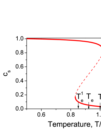
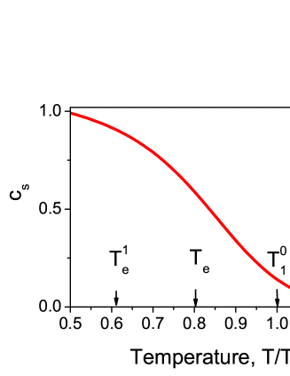
Figure 1: (Color online) The solid-like fraction of of liquid, $c_{s}$, vs $T/T_{e}^{0}$ at (a) $\tilde{g}_{sf}\left({P,T_{e}}\right)>2T_{e}$ and (b) $\tilde{g}_{sf}\left({P,T_{e}}\right)<2T_{e}$.

The temperature $T_{e}$, at which the ‘‘external field’’ $h_{sf}$ is equal to zero, is the coexistence temperature of two heterophase liquid states determined by equation

$$g_{f}^{0}\left(P,T_{e}\right)=g_{s}^{0}\left(P,T_{e}\right)+g_{ss}/2.$$ (7.10)

At $T=T_{e}$, we have $c_{s}(T_{e})=c_{f}(T_{e})=1/2$. In the vicinity of $T_{e}$,

$$c_{s}\approx\frac{1}{2}+\frac{h_{sf}(T)}{2(2T_{e}-\tilde{g}_{sf})}\left[1-\frac{2Th_{sf}^{2}(T)}{3(2T_{e}-\tilde{g}_{sf})^{3}}\right]=\frac{1}{2}+\frac{\Delta s_{s,f}(T_{e})\left(T-T_{e}\right)}{2(2T_{e}-\tilde{g}_{sf})}+O\left((T-T_{e})^{3}\right).$$ (7.11)

As it follows from (7.7), (7.9) and (7.10),

$$T_{e}^{0}\approx T_{e}+g_{ss}/2\Delta s_{f,s}\,,\qquad T_{e}^{1}\approx T_{e}-g_{ss}/2\Delta s_{f,s}\,.$$ (7.12)

The solution (7.11) is stable at $\tilde{g}_{sf}\left(P,T_{e}\right)<2T_{e}$. If $\tilde{g}_{sf}\left(P,T_{e}\right)>2T_{e}$, it is unstable and at $T=T_{e},(P)$ the first order phase transition takes place.

Graphic representation of solutions of equation (7.2) is shown in figure 1. The stable and unstable solutions are depicted by solid and dashed lines, respectively.

If $\tilde{g}_{sf}=2T_{e}$, i.e.

$$g_{ss}=2g_{sf}-4T_{e}\,,$$ (7.13)

then, the 2nd order phase transition takes place at $T=T_{e}(P)$. In accordance with (7.5) and (7.8), above $T_{e}^{0}$ and below $T_{e}^{1}$, the HPF are weak but within the temperature range $\left[T_{e}^{1},T_{e}^{0}\right]$, where in compliance with (7.11) $c_{s}$ and $c_{f}$ are comparable quantities, they are strong.

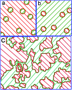
Figure 2: (Color online) Schematic representation of the hetrophase liquid states: (a) rare $s$-fluctuons in fluid described by equation (7.5); (b) $f$-fluctuons in glass [equation (7.8)]; (c) heterophase state with comparable fractions of the $s$- and $f$-fluctuons [equation (7.11)].

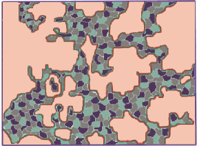
Figure 3: (Color online) The same as in figure 2 (c) but the mesoscopic structure of the solid-like fraction containing several types of the $s$-fluctuons is shown.

It worth to note that the solutions (7.5) and (7.8) reproduce the results of Frenkel’s model in the vicinity of the phase coexistence temperatures (here, $T_{e}^{0}$ and $T_{e}^{1}$, respectively). Therefore, $T_{e}^{0}$ can be considered as the coexistence temperature of the fluid and heterophase liquid phases while $T_{e}^{1}$ is the phase coexistence temperature of the ‘‘ideal’’ glass (as it is determined above) and the heterophase liquid. Thus, $T_{e}^{1}$ is the ideal glass transition temperature. The real glass transition temperature, $T_{\textrm{g}}$, which depends on $\tau_{\textrm{obs}}$ (see section 3), is above $T_{e}^{1}$ due to dramatic retarding of the structure relaxation with temperature decrease. For this reason, the real glass transition temperature range, $\left[T_{\textrm{g}},T_{e}^{0}\right]$, is narrower than $\left[T_{e}^{1},T_{e}^{0}\right]$. The structure of the heterophase states in the vicinity of the characteristic temperatures $T_{e}^{1}$, $T_{e}$ and $T_{e}^{0}$ is schematically presented in figure 2. In figure 3, the mesoscopic structure of the solid-like fraction with several types of $s$-fluctuons is shown schematically. Let us remind that the solutions of equations (7.5), (7.8), (7.11) are obtained under the assumption that the fractions of $s$-fluctuons $\left\{c_{i}\right\},i=1,\ldots,m$ are nearly constant or they are changing continuously and smoothly. This assumption fails if a phase transformation with stepwise changes of the fractions $\left\{c_{i}\right\}$ within the solid-like fraction takes place. In the next section, the impact of such a phase transformation within the solid-like fraction on the features of the fluid-solid phase transformation is considered.

7.2 Phase transition in the solid-like fraction

Evidently, a phase transition in the solid-like fraction causes a non-analytic behaviour of the solutions of equation (7.2). This type of the liquid-liquid transition appears due to multiplicity and interaction of the $s$-fluctuons which leads to the mutual ordering and phase separations within the solid-like fraction.

As a minimal model, let us consider the heterophase liquid with two types of $s$-fluctuons. Hence, $m=2$. Thus, in (6.3) $i,j=1,2$. The equation of state (6.3) for the solid-like fraction is as follows:

$$\left(1-2c_{1}^{*}\right)c_{s}\tilde{g}_{12}+T\ln\frac{c_{1}^{*}}{1-c_{1}^{*}}=h_{12}\,,\qquad c_{i}^{*}=c_{i}/c_{s}\,,\qquad c_{1}^{*}+c_{2}^{*}=1\,,$$

$$\tilde{g}_{12}=g_{12}-\left(g_{12}+g_{22}\right)/2,\qquad h_{12}=g_{2}^{0}-g_{1}^{0}+c_{s}\left(g_{22}-g_{11}\right)/2.$$ (7.14)

It is seen that this equation is isomorphic to equation (7.2) but the ‘‘external field’’ $h_{12}$ and the pair interaction coefficient $c_{s}\tilde{g}_{12}$ depend on $c_{s}$. Therefore, associated solutions of equations (7.2) and (7.14) should be considered together. The search for a general solution of these nonlinear equations at an arbitrary set of coefficients is a cumbersome and hardly attractive task because the values of the coefficients for substances are initially unknown. Nevertheless, we can look for some ‘‘typical’’ solutions at a reasonable specification of the coefficients.

As a useful example, let us consider solutions of equation (7.14) in the vicinity of the coexistence curve, $h_{12}\left(P,T\right)=0$, assuming that $c_{s}\left(g_{22}-g_{11}\right)$ is a negligible quantity. In this case, the coexistence temperature, $T_{12}$, is determined by equation

$$g_{1}^{0}\left(P,T_{12}\right)=g_{2}^{0}\left(P,T_{12}\right).$$ (7.15)

     

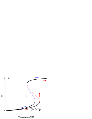
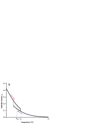
Figure 4: (Color online) First order phase transition within the solid-like fraction (a) induces the liquid-liquid first order phase transition (b).

It is assumed that $T_{12}$ is above the coexistence temperature $T_{e}$. A phase transformation of the solid-like fraction and induced liquid-liquid phase transition at $T_{12}<T_{e}$ is considered in [27].

In the vicinity of $T_{12}$

$$h_{12}=g_{1}^{0}\left(P,T\right)-g_{2}^{0}\left(P,T\right)\approx\left(s_{1}-s_{2}\right)\left(T-T_{12}\right)\equiv\Delta s_{12}{\kern 1.0pt}\left(T-T_{12}\right),$$ (7.16)

$s_{1}$ and $s_{2}$ is the entropy of $s$-fluctuon of type 1 and 2, respectively.

If $c_{s}\left(T_{12}\right)\tilde{g}_{12}>2T_{12}$, then there are two stable solutions of equation (7.14) and, as a consequence, two stable solutions of equations (7.2), (7.3). Consideration of these solutions is contained in appendix B. Their graphic representation is shown in figure 4. The jump of the parameter $c_{s}$ at $T=T_{12}$ is [see (B.7) in appendix B] as follows:

$$\Delta c_{s}\left(T_{12}\right)\approx\left(s_{1}-s_{2}\right)\exp\left(-g_{sf}\beta\right).$$ (7.17)

     

Figure 5: Continuous but stepwise evolution of $c_{1}^{*}\left(T\right)$shown in a) induces the appearance of the inflection point of $c_{s}\left(T\right)$ at $T=T_{12}$, b).

If $c_{s}\left(T_{12}\right)\tilde{g}_{12}<2T_{12}$, the fractions $c_{1}^{*},c_{2}^{*}$ and parameter $c_{s}$ change continuously at $T=T_{12}$ but the inflection points of the functions $c_{1}^{*}\left(T\right)$ and $c_{s}\left(T\right)$ appear at $T=T_{12}$ (figure 5). Hence, the expression (7.17) estimates the bench height of the parameter $c_{s}$.

The heat of the phase transitions is determined by equation (B.8) in appendix B,

$$\Delta H_{12}\simeq c_{s}\left(T_{12}\right)(s_{1}-s_{2})k_{0}^{-1}\left[H_{fs}+T_{12}\right],$$ (7.18)

$H_{fs}$ is the heat of the fluid-solid phase transition. It is taken into account here that the heat of $1\leftrightarrow 2$ solid-solid phase transition is equal to $(s_{1}-s_{2})k_{0}^{-1}T_{12}$.

It is worth to note that at a fixed value of $c_{s}$, equation (7.14) is isomorphic to Ising model with non-zero external field and with exchange integral $c_{s}\tilde{g}_{12}$ which can be positive or negative. The external field controls the ratio $c{}_{1}^{*}/c{}_{2}^{*}$ while the sign of the exchange integral determines the type of mutual ordering of the $s$-fluctuons. With $c_{s}\tilde{g}_{12}>0$ (ferromagnetic interaction), $s$-fluctuons of different types tend to separate. At $c_{s}\tilde{g}_{12}<0$, the ‘‘antiferromagnetic’’ order with alternating $s$-fluctuons of different types is preferable. In both cases, the fluctuonic SRO generates molecular medium-range order with the correlation length $\xi_{fl}\sim 2r_{0}$ [in compliance with the general conclusion made in section 4 after equation (4.6)].

7.3 The Fischer cluster

Along with the above considered types of MRO appearing due to local fluctuonic interaction, there is a different type of the fluctuonic order with comparatively large (as it was observed, up to $\sim 102$ nm) correlation length, $\xi_{\textrm{FC}}\gg\xi_{fl}$. It appears due to the aggregation of the $s$-fluctuons under the effect of the volumetric gravitation potential (4.6). The equilibrated aggregation of $s$-fluctuons possesses the fractal structure with fractal dimension, correlation length, equilibration time and relaxation dynamics depending on the liquid features and temperature. This remarkable phenomenon, which was discovered and investigated in detail by Fischer et al. [1, 2, 3, 4, 5, 6, 7, 8, 9, 10, 23, 24, 25, 26, 27], is known as the Fischer cluster. The Fischer cluster was visualized by observing a speckle pattern in ortho-terphenil [6]. The speckle pattern fluctuates and rearranges very slowly, with characteristic time $\sim 1$ min at $T=293$ K, while the $\alpha$-relaxation time at this temperature is $\tau_{\alpha}=40$ ns. With temperature increase, the speckle size and contrast decreases and at $T>340$ K no speckle is seen. Schematically, the heterophase liquid structure with and without the Fischer cluster is shown in figure 6. It is worth to note that the Fischer cluster formation in heterophase liquid is not an exclusion but the rule if the Fischer cluster equilibration time, $\tau_{\textrm{FC}}$, is shorter than the observation time, i.e., if $\tau_{\alpha}\ll\tau_{\textrm{FC}}\ll\tau_{\textrm{obs}}\ll\tau_{\textrm{LRO}}$. The heterogeneous structure and slow structural relaxation are observed not only in many Van der Waals molecular liquids but also in some metallic melts above $T_{m}$ [58, 59, 60].

The Fischer cluster was originally identified using the results of the small-angle X-ray scattering on the density fluctuations. The conventional large-scale density fluctuations in a homophase liquid are proportional to the isothermal compressibility $\kappa_{T}$ and are independent of the wave vector $q$,

$$\left|\rho(q)\right|^{2}\left.\right|_{q\to 0}\sim\kappa_{T}T.$$ (7.19)

Here, $q$ is the wave vector, $\rho(q)$ is the amplitude of density fluctuations. The intensity of X-ray scattering on the density fluctuations, $I\left(q\right)$, is proportional to $\left|\rho(q)\right|^{2}$.

It appears that a $q$-dependent excess scattering intensity, $I_{\textrm{exc}}\left(q\right)\sim q^{-D}$ ($D$ is the fractal dimension) occurs at $T<T_{A}\approx T_{e}^{0}$. The $I_{\textrm{exc}}\left(q\right)$ is much larger than the scattering intensity on the thermal fluctuations (7.19). The results of the wide-angle X-ray scattering show that SRO of the liquid contains both the fluid-like and solid-like components at $T<T_{A}$ [9, 61]. It turns out that the thermodynamics and $\alpha$-relaxation dynamics are quite the same in the liquid states with and without the Fischer cluster. It means that the changes of the thermodynamic properties due to the Fischer cluster formation are too small to be reliably detected and that the fluctuonic SRO does not undergo noticeable changes. Therefore, the Fischer cluster formation can be considered as the process of self-organization of the correlated domains (CDs), i.e., entities possessing the fluctuonic SRO with the correlation length $\xi_{fl}\approx 2r_{0}$, (section 4).

Theory of the Fischer cluster is developed in [10, 23, 24, 25, 26]. The Fischer cluster is considered as a fractal aggregation of $s$-fluctuons with the fractal dimension $D_{f}$ and correlation length $\xi_{\textrm{FC}}$. Minimization of the free energy as function of $\bar{c}_{s}$, $D_{f}$ and $\xi_{\textrm{FC}}$ allows one to determine the equilibrium values of $D_{f}$ and $\xi_{\textrm{FC}}$. It is found (see appendix C) that

$$\xi_{\textrm{FC}}\left(\overline{c}_{s},D_{f}\right)\approx\left(\overline{c}_{s}\right)^{\frac{1}{D_{f}-3}}r_{0}\,,\qquad D_{f}=3-\left(\ln\frac{r_{0}}{\xi_{fl}}\right)^{-1}\ln c_{s,\textrm{CD}}\,,$$ (7.20)

$c_{s,\textrm{CD}}$ is the concentration of $s$-fluctuons within CD ([24, 25, 26], appendix C)

$$c_{s,\textrm{CD}}=\left[1+\frac{I(D_{f},\xi_{\textrm{FC}})}{\partial^{2}g^{0}\left(\overline{c}_{s}\right)/\partial\overline{c}_{s}^{2}-I(D_{f},\xi_{\textrm{FC}})}\right]\overline{c}_{s}\geqslant\overline{c}_{s}\,.$$ (7.21)

The quantity $I(D_{f},\xi)$, (C.21), is proportional to $\phi_{0}$. Equation (7.21) shows that within the CD, concentration of $s$-fluctuons is larger than its mean value $c_{s}$: $c_{s,\textrm{CD}}\simeq c_{s}+\textrm{const}\,\phi_{0}$.

The liquid state with the Fischer cluster is stable (while the state without the Fischer cluster is metastable or unstable) at

$$c_{s}>c_{s,0}<\left(\frac{r_{0}}{\xi_{fl}}\right)^{2}\approx 0.16,\qquad 1<D_{f}\leqslant 3.$$ (7.22)

     

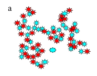
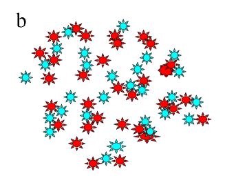
Figure 6: (Color online) Schematic fragments of the heterophase liquid with (a) and without (b) Fischer’s cluster. Just two types of statistically significant $s$-fluctuons are shown. The circle shows the size of the correlated domain.

Transformation of the state without Fischer’s cluster into the state with Fischer’s cluster is a weak first order phase transition with the transformation heat $\propto\varphi_{0}$.

The upper bound of the $c_{s}$-range in which the Fischer cluster exists, $c_{s,1}=(\xi_{fl}/r_{0})^{2}c_{s,0}$ [see (C.26)], decreases, $\sim\phi_{0}$, with an increase of the strength of the $s$-fluctuons gravitation potential $\phi_{0}$. When $c_{s}$ approaches $c_{s,1}<1$ from below, the fractal dimension $D_{f}{\kern 1.0pt}{\kern 1.0pt}$ approaches 3 and $\xi_{\textrm{FC}}\to\infty$. It means that at $c_{s}\geqslant c_{s,1}$ the solid-like fraction consists of the connected 3-dimensional solid-like clusters of size $r>\xi_{fl}$. Thus, at $c_{s}\geqslant c_{s,1}$, the topology of the heterophase liquid equilibrated on scale $r\geqslant\xi_{fl}$ changes.

7.4 Parametric phase diagram

In the HPFM, the structure and phase states of the heterophase liquid are described in terms of $T$ and coefficients $g_{sf}$, $g_{ss}$, $h_{sf}$. It is useful to construct a phase diagram (the parametric phase diagram) of the glass-forming liquid in terms of these parameters. The parametric phase diagram of the two-state approximation is determined by equations (7.7), (7.9), (7.10) and the equation (7.22) in combination with (7.5). Namely, they determine the coexistence temperatures of different states in terms of the coefficients $g_{sf},g_{ss},h_{sf}$. The quantities $T_{e}^{0},T_{e}^{1}{\kern 1.0pt},T_{e}{\kern 1.0pt}{\kern 1.0pt}{\kern 1.0pt}{\kern 1.0pt}{\kern 1.0pt}$and $T_{\textrm{FC}}$ are coexistence temperatures of

1. the fluid and heterophase liquid ($T_{e}^{0}$);

2. the heterophase liquid and ‘‘ideal’’ glass($T_{e}^{1}$);

3. the fluid-like and solid-like states ($T_{e}$);

4. the heterophase liquid with and without the Fischer cluster ($T_{\textrm{FC}}$).

Introducing the scaled temperature, $T^{*}=T/T_{e}^{0}$, and the frustration parameter $g_{ss}^{*}=g_{ss}/\Delta s_{f,s}T_{e}^{0}$, we can present the relations (7.8) in a dimensionless form,

$$T_{e}^{0*}=1,\qquad T_{e}^{*}=1-g_{ss}^{*}/2,\qquad T_{e}^{1*}\approx 1-g_{ss}^{*}\,.$$ (7.23)

The end critical point location on the fluid-solid phase coexistence curve, $T^{*}=T_{e}^{*}\left(P\right)$ is located at

$$g_{ss,\textrm{c}}^{*}={2g_{sf}\mathord{\left/{\vphantom{2g_{sf}\left(\Delta s_{s,f}T_{e}^{0}\right)}}\right.\kern-1.2pt}\left(\Delta s_{s,f}T_{e}^{0}\right)}-4T_{e}^{*}\left(P\right)>0.$$ (7.24)

The first order fluid-solid phase transition on the phase coexistence curve takes place at $g_{ss}^{*}<g_{ss,\textrm{c}}^{*}$.

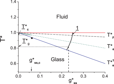
Figure 7: (Color online) Parametric phase diagram on the plane $\left(T^{*},g^{*}_{ss}\right)$, $T^{*}=T/T_{e}^{0}$, $g^{*}_{ss}=g_{ss}/\Delta s_{s,f}T_{e}^{0}$. The phase coexistence lines $T=T_{e}^{0}$; $T=T_{e}$; $T=T_{e}^{1}$ and the threshold of the Fischer cluster formation temperature, $T_{\textrm{FC}}^{*}$, approximately determined using equations (7.5), (7.22) are shown. The critical end point at $g_{ss,\textrm{c}}^{*}$ exists on the line $T=T_{e}$. Bold line 1 schematically presents an evolution phase curve of the equilibrium system.

The parametric phase diagram depicted on the plane $\left(T^{*},g_{ss}^{*}\right)$ using relations (7.23), (7.24) and (7.22), (7.5) is shown in figure 7. As an example, here is also shown one phase trajectory which becomes non-physical below the glass transition temperature $T_{\textrm{g}}^{*}$. Within the range $0<g_{ss}^{*}<g_{ss,\textrm{c}}^{*}$ the first order phase transition takes place on the phase coexistence line $T^{*}=T_{e}^{*}$. A weak first order phase transition takes place on the line $T^{*}=T_{\textrm{FC}}^{*}$.

7.5 Static structure factor and the order parameter restoration

Pair correlation function of the density fluctuations , $\stackrel{{\scriptstyle\frown}}{{\varpi}}(q,T)$, of the heterophase liquid with the Fischer cluster is $\sim q^{-D}$ at $r_{0}\ll q^{-1}\ll\xi^{-1}$. At $qr_{0}\sim 1$, it is a superposition of the pair correlation functions of fluctuons,

$$\stackrel{{\scriptstyle\frown}}{{\varpi}}(q,T)=c_{f}(T)\varpi_{f}(q)+\sum_{i=1}^{m}c_{i}(T)\varpi_{i}(q)=\left[1-c_{s}(T)\right]\varpi_{f}(q)+c_{s}(T)\varpi_{s}(q),$$ (7.25)

$$\varpi_{s}(q)=\frac{1}{c_{s}}\sum_{i=1}^{m}c_{i}\varpi_{i}(q),$$ (7.26)

$\varpi_{f}(q)$, $\varpi_{i}(q)$ are Fourier transforms of the pair correlation functions of the $f$- and $s$-fluctuons, respectively. The cross-correlation terms $\sim c_{f}c_{s}$ are omitted in (7.25). The quantities $\varpi_{f}(q)$, $\varpi_{i}(q)$ weakly depend on the temperature. For this reason, the equation (7.25) can be applied to restore the order parameter $c_{s}(T)$ using the structure factors $\varpi_{f}(q)$, $\varpi_{s}(q)$ measured in the liquid, fluid and glassy states [61]. On the other hand, as it is shown in [22], $c_{s}(T)$ can be restored from calorimetric data using the relation

$$c_{s}\simeq\left[H_{f}(T)-H_{\exp}(T)\right]/\left[H_{f}(T)-H_{s}(T)\right]$$ (7.27)

which follows from equation (4.3). Here, $H_{f}(T),H_{s}(T)$ are enthalpies of the fluid and glass extrapolated in the temperature range $\left[T_{e}^{1},T_{e}^{0}\right]$, and $H_{\exp}(T)$is the experimentally measured enthalpy of the glass-forming liquid. Comparison of the results of the order parameter restoration from the structural data, using equation (7.25), and from the calorimetric data, using relation (7.27), gives a good chance to check the reliability of the HPFM. This procedure was performed using structural and calorimetric data of salol [9, 61]. Results are presented in figure 8 by scattered symbols. Solution of the equation of state in the two-state approximation (subsection 7.1), in which the experimentally measured thermodynamic parameters and free parameter $\tilde{g}_{sf}$ are used, is presented there by a solid line.

Let us remind that the analytic solution describes the order parameter $c_{s}(T)$ of the equilibrated system. Therefore, it noticeably deviates from the experimentally determined values $c_{s}(T)$ near the glass transition temperature, where the liquid becomes non-equilibrium. Relations (7.25) and (7.27), obtained without the assumption that the system is equilibrated, allow us to recover the thermal history of ‘‘true’’ (in the phenomenological sense) value of $c_{s}$.

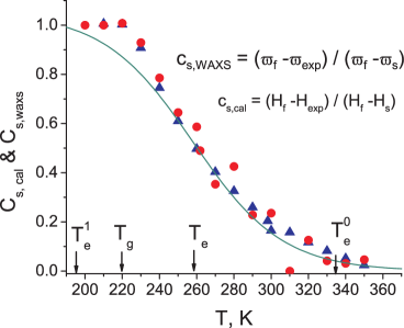
Figure 8: (Colo online) The solid-like fraction of salol vs $T$ as it is found from the analysis of the calorimetric data (triangles), and from the temperature dependence of the structure factor (circles) [22, 61]. Arrows indicate the temperatures $T_{e}^{0}$, $T_{e}$, $T_{\textrm{g}}$, $T_{e}^{1}$. Line presents an analytic solution of the equation of state in the two-state approximation with fitting parameter $\tilde{g}_{sf}$.

8 Dynamics

8.1 $\alpha$-relaxation

Thermally activated cooperative structural rearrangements which can involve up to $\sim 10^{2}$ molecules [19, 20, 63, 64, 65, 66, 67] are called $\alpha$-relaxation. A large amount of the molecules are involved in the rearrangement due to correlations. Structural rearrangement of a fluctuon also involves rearrangements of the neighboring fluctuons within CD of size $\xi_{fl}$. Therefore, the size of cooperatively rearranging domain is nearly equal to $\xi_{fl}$.

The activation energy of $\alpha$-relaxation,

$$E_{\textrm{ac}}=\frac{d\ln\tau_{\alpha}}{d\beta}\,,\qquad\beta=\frac{1}{T}\,,$$ (8.1)

depends on the order parameter. It can be presented as an expansion in powers of the order parameter [10, 22],

$$E_{\textrm{ac}}=E_{\textrm{ac}}^{0}+E_{\textrm{ac}}^{1}c_{s}+E_{\textrm{ac}}^{2}c_{s}^{2}+\ldots\;.$$ (8.2)

Above $T_{A}$, the activation energy is nearly equal to $E_{\textrm{ac}}^{0}$. Cooperativity of the liquid dynamics is induced by the $s$-fluctuons interaction which becomes considerable below $T_{A}$.

Fischer and Bakai [22] have suggested that CD can be rearranged when all the molecules therein are in fluid-like state with correlations destroyed on the scale $\xi_{fl}$. This assumption leads to the following expression [22]

$$E_{\textrm{ac}}=\frac{A}{\left(1-T_{\textrm{K}}/T\right)^{2}}+z_{\textrm{CD}}c_{s}\left(H_{f}-H_{s}\right)+O\left(c_{s}^{2}\right).$$ (8.3)

$z_{\textrm{CD}}\sim\left(\xi_{fl}/a\right)^{3}$ is the cooperativity parameter, which is the mean n umber of molecules within the CD; $H_{f}$, $H_{s}$ is the enthalpy of liquid-like and solid-like fraction per molecule. The first term is taken in the form proposed for random packings of spheres in [68, 69]. Its denominator takes into account the decrease of the free volume of the fluid and the numerator is equal to the activation energy above $T_{A}$. The Kauzmann temperature, $T_{\textrm{K}}$, is a fitting parameter (see comments concerning $T_{\textrm{K}}$ in section 3)

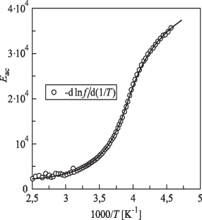
Figure 9: The activation energy of salol vs the reciprocal temperature [2].

Enthalpies $H_{f}\left(T\right)$ and $H_{s}\left(T\right)$ within the temperature range $\left[T_{\textrm{g}},T_{A}\right]$ are understood as extrapolations of these functions measured at $T>T_{A}$ and $T<T_{\textrm{g}}$, respectively.

As an example of using the equation (8.3) [22], the activation energy of salol was analyzed in [22]. The activation energy of salol vs the reciprocal temperature is shown in figure 9. The experimental data are shown by circles. The curve is a result of fitting the formula (8.3) using parameters $A=967$ K; $T_{\textrm{K}}=153$ K, $T_{e}=257$ K; $T_{A}\approx 325$ K; $z_{\textrm{CD}}=32$; $k_{0}=7$. The input of the first term of r.h.s of (8.3) in the activation energy is nearly 10% at $T=T_{\textrm{g}}$.

It is noteworthy that since the main input in the activation energy makes the term proportional to $c_{s}$, $E_{\textrm{ac}}\left(T\right)$ has the inflection point at $T\approx T_{e}$. Stickel has proposed an efficient method of analysing the $\alpha$-dynamics to check the applicability of the Vogel-Fulcher-Tamman formula and other phenomenologic and empiric expressions proposed for $\tau_{\alpha}(T)$ [70, 71, 72]. He has analyzed many molecular liquids and found the flex points of $E_{\textrm{ac}}\left(T\right)$ identified as $T_{e}$. Coincidence of the values of $T_{A}$ and $T_{e}$ extracted from the dynamic, calorimetric and structural data (figures 8, 9) support the adequacy of HPFM.

8.2 Ultra-slow modes and the Fischer cluster equilibration time

Two relaxational modes are connected with the Fischer cluster. The phase transformation of a liquid without the Fischer cluster into the state with the cluster is controlled by nucleation and growth of a new phase. Since the phase transformation heat is small, the phase equilibration time is rather large compared with the time of elementary cooperative rearrangement $\tau_{\alpha}$. The Fischer cluster equilibration time is determined in [10],

$$\tau_{\textrm{FC}}\sim\frac{T}{\varphi}\left(\frac{\xi_{\textrm{FC}}}{\xi_{fl}}\right)^{D_{f}+2}\frac{\tau_{\alpha}}{D_{f}-1}\,.$$ (8.4)

Rearrangements of the equilibrated Fischer cluster on the scales $\xi_{fl}^{-1}\gg q>\xi_{\textrm{FC}}^{-1}$ are registered as the ultra-slow modes [2, 3, 4, 5, 6, 7, 8, 9]. The relaxational rate of the ultra-slow mode is $\sim q^{2}$. It is found within the framework of HPFM [10] that

$$\Gamma_{\textrm{usv}}\left(q\right)\sim\left(q\xi_{\textrm{FC}}\right)^{2}\left(\frac{\pi\xi_{fl}}{\xi_{\textrm{FC}}}\right)^{2}\tau_{\alpha}^{-1}+O\left(q^{4}\right).$$ (8.5)

The characteristic times $\Gamma_{\textrm{usv}}^{-1}$ and $\tau_{\textrm{FC}}$ are proportional to $\tau_{\alpha}$ and the proportionality coefficients are rather large at $\xi_{\textrm{FC}}\gg\xi_{fl}$. As it is seen, $\tau_{\textrm{FC}}\gg\Gamma_{\textrm{usv}}^{-1}\gg\tau_{\alpha}$. Relations (8.4),(8.5) are in harmony with the experimental data.

8.3 Fragility

The fragility parameter, $\stackrel{{\scriptstyle\frown}}{{m}}$, introduced by Angell in [73, 74], is an important characteristic of the glass-forming liquid dynamics near $T_{\textrm{g}}$. It is taken as the measure of deviation of the temperature dependence of $\tau_{\alpha}$ from the Arrhenius law. There exist strong liquids, with small fragility parameter, $\stackrel{{\scriptstyle\frown}}{{m}}\;\sim 10$, the most fragile liquids, with $\stackrel{{\scriptstyle\frown}}{{m}}\;\approx 10^{2}$, and liquids with moderate fragility in between. The fragility parameter is tightly connected with the structural properties and thermodynamics of a liquid, and for this reason, it is widely used at analysing the glass transition and classification of liquids. Angell’s definition of this parameter is as follows:

$$\stackrel{{\scriptstyle\frown}}{{m}}=T_{\textrm{g}}^{-1}\left[\frac{\mathrm{d}\left(\log\tau_{\alpha}\right)}{\mathrm{d}\beta}\right]=\left.\frac{E_{\textrm{ac}}}{T_{\textrm{g}}\ln 10}\right|_{T_{\textrm{g}}}.$$ (8.6)

In HPFM, the quantity $E_{\textrm{ac}}$ is determined by equation (8.3). As it follows from (8.3) and (8.6),

$$\stackrel{{\scriptstyle\frown}}{{m}}=\frac{1}{T_{\textrm{g}}}\left[\frac{A}{\left(1-T_{\textrm{K}}/T_{\textrm{g}}\right)^{2}}+z_{\textrm{CD}}\left[H_{f}(T_{\textrm{g}})-H_{s}(T_{\textrm{g}})\right]k_{0}^{-1}c_{s}\left(T_{\textrm{g}}\right)\right],$$ (8.7)

$$H_{f}\left(T_{\textrm{g}}\right)-H_{s}\left(T_{\textrm{g}}\right)\sim\left(s_{f}-s_{s}\right)\left(T_{\textrm{g}}-T_{e}\right).$$

The main contribution in $\stackrel{{\scriptstyle\frown}}{{m}}$ gives the second term within the brackets of (8.7). It is proportional to the number of molecules involved in the cooperative rearrangement, $z_{\textrm{CD}}\sim\xi_{fl}^{3}$, as well as to the difference of the configurational entropies of the solid-like and fluid-like species. The difference of their vibrational entropies is comparatively small. Since these quantities can be measured regardless of $\tau_{\alpha}$, equation (8.7) permits to check the relevance of the HPFM predictions. For example, it was found that for salol, HPFM gives $\stackrel{{\scriptstyle\frown}}{{m}}\;\approx 67$ [10]. The fragility parameter of salol estimated in [75] is equal to 63.

As it was noted above, (subsection 8.3), the $H_{f}\left(T\right)$ and $H_{s}\left(T\right)$ within the temperature range $\left[T_{\textrm{g}},T_{A}\right]$ are understood as extrapolations of these functions measured at $T>T_{A}$ and $T<T_{\textrm{g}}$, respectively. Naturally, the linear or quadratic extrapolation provides an acceptable result if the function is smooth and the higher derivatives are small. Phase transformations in the solid-like fraction lead to stepwise changes of $H_{s}\left(T\right)$and, consequently, to the stepwise behavior of $\tau_{\alpha}\left(T\right)$. In this case, extrapolations of $\tau_{\alpha}\left(T\right)$, determined by equation (8.1), from high and low temperatures into the range $\left[T_{\textrm{g}},T_{A}\right]$ cannot be properly fitted. Equations (7.17), (7.18), (8.1)–(8.3) determine the temperature dependence of $\tau_{\alpha}\left(T\right)$ in this case.

In a series of experiments with some metallic glasses [76, 77, 78, 79, 80], the fragility parameter value determined using the data on $\tau_{\alpha}\left(T\right)$ in the vicinity of $T_{\textrm{g}}$ and its value recovered from the extrapolated curve $\tau_{\alpha}\left(T\right)$ measured at high temperatures are completely different. As it is revealed [76], such a behavior of $\tau_{\alpha}\left(T\right)$ of Zr-based alloy Vitreloy 4 is connected with the liquid-liquid first order phase transition. In others melts, a transition of this type is assumed.

Equations (7.17), (7.18), (8.1)–(8.3) provide theoretical description of this phenomenon known as the fragile-to-strong liquid transformation. More in detail it is considered in [81].

9 Concluding remarks

The statistical basics of HPFM include substantiation of the mesoscopic efficient Hamiltonian and the application of the bounded statistics method while describing supercooled liquid states. Solutions of the equations of state of HPFM ascertain interplay of the thermodynamic, structural and dynamic properties of the glass-forming liquids. Thus, juxtaposing the theoretical predictions with experimental data (as an example, see figures 8, 9) permits to cross-verify the adequacy of HPFM.

The conditions of the liquid quasi-equilibrium evolution (3.1), (3.2) determine the applicability range of the bounded statistics in which the states with the crystalline order on scale $\xi\gg\xi_{fl}$ are excluded. On the other hand, the amorphous states with the fluctuonic order having large correlation length are included in the statistics and the Fischer cluster is described within the framework of HPFM. Compatibility of the conditions (3.1), (3.2) with the fluctuonic order equilibration on large scales should be specified.

The hierarchy of characteristic scales of spatial correlations (starting from the local order and molecular size a), $a<\xi_{\textrm{SRO}}<\xi_{fl}<\xi_{\textrm{FC}},\ldots$ is connected with the hierarchy of time scales $\tau\left(a\right)<\tau_{\alpha}\left(\xi_{fl}\right)<\Gamma_{\textrm{usv}}^{-1}<\tau\left(\xi_{\textrm{FC}}\right)$ [$\tau\left(a\right)$ is the molecule oscillation time within the cage]. Elementary step of the nucleation and growth of the crystalline embryo is the cooperative rearrangement on the spatial and time scales $\xi_{fl}$ and $\tau_{\alpha}$, respectively. Therefore, the formation of the crystalline embryos with the size larger than $\xi_{fl}$ takes much longer time than the SRO equilibration time. As a result, the condition (3.2) can be regarded as satisfied when the condition (3.1) is fulfilled. Hence, the crystalline species of size $\sim\xi_{fl}$ coexist with non-crystalline species within the solid-like fraction of liquid and in glass. As a confirmation, direct observations of the structure of metallic glasses by means of a high resolution field ion microscopy and transmission electron microscopy (see figure 6.5 in [21], [82, 83] and references cited) reveal the coexistence of crystalline and non-crystalline structural species with sizes of up to a few nanometers.

The Fischer cluster equilibration (along with the ultra-slow modes) is observable only if the crystallization time is much longer than $\tau\left(\xi_{\textrm{FC}}\right)$. The crystallization heat (which is the thermodynamic driving force of the crystallization) is much larger than the heat of the Fischer cluster formation. Therefore, the Fischer cluster can be observed just in normal liquids and in the supercooled liquids with strongly hindered crystallization.

The amount of the solid-like fraction, $c_{s}$, determines the measure of the fluid-to solid transformation. Due to the definitive role of $c_{s}\left(T\right)$, its description is an important issue of the theory. The two-state approximation is a minimal model permitting to solve this problem considering the fluid-solid HPF states without details of the solid-like subsystem. Evidently, this model is satisfactory if just one type of the $s$-fluctuons is statistically significant or when variations of the probabilities $\left\{c_{i}^{*}\right\}$ within the glass-transition temperature range are insignificant, i.e., if the mesoscopic structure of the solid-like fraction does not vary considerably. At the same time, estimation of the two-state approximation accuracy shows that it can yield acceptable results in more general cases.

The accuracy of the two-state approximation can be estimated considering the states with transforming $s$-fluctuons. The assumption on a smooth evolution of the coefficients of equation (7.2) fails if the phase transformations, similar to those considered in subsection 7.2, take place within the solid-like fraction. Nevertheless, even in this case, a stepwise jump of $c_{s}\left(T\right)$ is comparatively small because the entropy jump and transformation heat at the solid-solid polymorphic transformation, as a rule, is small, $\Delta s_{12}\sim 10^{-1}$ while $\Delta s_{fs}\sim 1$. Therefore, one can expect that the two-state approximation is acceptable with accuracy to terms $O\left(10^{-1}c_{s}\right)$ or even better.

Figuratively speaking, in a general case, the glass and solid-like fraction of a liquid is a mosaic composed by the mesoscopic species of size $\sim r_{0}$ (figure 3). However, unless until the mutual ordering of $s$-fluctuons and the impact of the mosaic details on $c_{s}$ is beyond the scope of interests, the two-state approximation can be used.

The question whether glass is a non-equilibrated highly viscous liquid or it is a non-equilibrated solid has rather got a conceptual sense. The thermodynamic continuity of the glass transition permits to believe that glass is a liquid with very high viscosity and long equilibration time. But, as a matter of fact, the glass near and below $T_{\textrm{g}}$, with $c_{s}\to 1$, is solid with statictically insignificant amount of the fluid-like species. Nevertheless, it flows, like a polycrystal does, due to the diffusional-viscous flow [84]. Field-emission microscopy of metallic glasses visualizes their grainy (polycluster) structure with sizes of grains $\sim 102$ nm. The Coble mechanism of the plastic deformation [85, 86] prevails near $T_{\textrm{g}}$ in such a glass [84]. The grainy structure of glass is the result of the existence of many centers of solidification within the liquid. Therefore, the polycluster mosaic structure of glass forms in liquids with different features of molecular forces. Slow structural relaxation hinders the ‘‘reclusterization’’ processes and the formation of ‘‘ideal’’ glass.

The Fischer cluster topology changes with an increase of the solid-like fraction. Its fractal dimension $D_{f}$ is less than 3 at $c_{s}<c_{s,1}$ and it is equal to 3 at $c_{s}\geqslant c_{s,1}$ (see subsection 7.3 and appendix C). Thus, at the point $c_{s}=c_{s,1}=1-\textrm{const}\;\phi_{0}$, the topological transition takes place at which the heterophase correlated domains transform into homophase ones. It is important that this transition does not presuppose the Fischer cluster equilibration on scales $\xi_{\textrm{FC}}>\xi_{fl}$. This result denotes a change of the structural relaxation mode at glass transition considered in [84].

The mesoscopic theory of thermodynamics and dynamics of the glass-forming liquids and glasses is connected with the microscopic approach based on the consideration of the potential energy landscape (see [87] and references cited) by the landscape coarsening procedure used while deducing the efficient Hamiltonian (appendix A). The coefficients of the fluctuon interaction save the memory on the microscopic potential energy landscape.

Appendix A The bounded phase space and efficient mesoscopic Hamiltonian

Below $T_{m}$, a crystalline state is the most probable one. It occupies a phase space region $\Omega_{\textrm{cr}}$ of the total phase space $\Omega$. $\Omega$ can be presented as the sum of the regions belonging to crystalline and non-crystalline states,

$$\Omega=\Omega_{\textrm{cr}}+\Omega_{\textrm{ncr}}\,.$$ (A.1)

Excluding $\Omega_{\textrm{cr}}$, we obtain the bounded phase space belonging to non-crystalline states. The bounded partition function

$$\stackrel{{\scriptstyle\frown}}{{Z}}\left(P,T\right)=\int_{\Omega_{\textrm{ncr}}}\exp\left[-E_{N}\left(x,p\right)\beta\right]\mathrm{d}^{3N}x\;\mathrm{d}^{3N}p$$ (A.2)

determines the free energy of the non-crystalline state

$$G\left(P,T\right)=-T\ln\stackrel{{\scriptstyle\frown}}{{Z}}\left(P,T\right).$$ (A.3)

In [39], the procedure of derivation of the equation of the free energy in terms of the order parameter (2.3), $G\left(\left\{c(x)\right\}\right)$, (it is called the efficient Hamiltonian in [39]) is expounded. It is based on the map of the phase space on the functional space of the order parameter $\left\{c\left(x\right)\right\}$,

$$G\left(\left\{c(x)\right\}\right)=-T\ln\int_{\Omega_{\textrm{ncr}}}\exp\left[-E_{N}\left(x,p\right)\beta\right]\prod_{\vec{q},i}\delta\big{(}c_{i}(\vec{q})-c_{i}(\vec{q};x,p)\big{)}\mathrm{d}^{3N}x\;\mathrm{d}^{3N}p.$$ (A.4)

Here, $c_{i}\left(\vec{q};x,p\right)$ are Fourier transforms of the components of the order parameter at a fixed coordinate $(x,p)$ of the bounded 6N-dimensional phase space $\Omega_{\textrm{ncr}}$.

Performing the integration in the functional space, we have

$$G\left(P,T\right)=-T\ln\int\exp\left[-G\left(\left\{c(\vec{q})\right\}\right)\beta\right]\prod_{\vec{q},i}\mathrm{d}c_{i}\left(\vec{q}\right).$$ (A.5)

Selecting in this expression the contribution of long-wavelength components, $q\to 0$, and performing a polynomial expansion in powers of $c_{i}\left(x\right)$ (4.1)–(4.6), we obtain

$$G\left(P,T\right) = -T\ln\int\exp\left[-H_{\textrm{eff}}\left(\left\{c\right\}\right)\beta\right]\prod_{qr_{0}\ll 1,i}\mathrm{d}c_{i}\left(\vec{q}\right)+\tilde{G}(P,T),$$

$$H_{\textrm{eff}}\left(\left\{c\right\}\right) = G\left(P,T;\left\{c(x)\right\}\right).$$ (A.6)

The term $\tilde{G}(P,T)$ takes into account the spatial fluctuations of the order parameter with $qr_{0}\sim 1$. To include this summand into consideration is important in the vicinity of critical points. It generates random fields and has an impact on criticality. It is shown in [10] that at the end point on the phase coexistence curve, the first order phase transition can take place due to the impact of the random field.

Within the framework of the method of cooperative variables, used while considering the gas-liquid critical point [88] and systems with the Ising-type Hamiltonian [89], a procedure of accounting of $\tilde{G}(P,T)$ in the vicinity of the critical point is expounded.

Appendix B Solutions of the equations of state

To get solutions of the equations (7.1)–(7.4), (7.14), (7.16), let us consider the solutions of equations (7.14), (7.16) taking $c_{s}\left(T\right)$ as an unknown function which should be determined later on using equations (7.2)–(7.4).

If $s_{1}>s_{2}$, the ‘‘external field’’ $h_{12}$ is positive below $T_{12}$ and negative above $T_{12}$. The first order phase transition takes place and discontinuous transformation of the phase 1 into phase 2 takes place at $T_{12}$ if

$$c_{s}\left(T_{12}\right)\tilde{g}_{12}>2T_{12}\,.$$ (B.1)

Under this condition, the solution similar to the solution (7.11) of equation (7.2) exists but it is unstable.

To get the other two solutions near $T_{12}$, equation (7.14) can be rewritten taking into account the relation (7.16) as follows:

$$-2\alpha^{*}c_{s}\tilde{g}_{12}+T\ln\frac{1+2\alpha^{*}}{1-2\alpha^{*}}\approx 2\left(-c_{s}\tilde{g}_{12}+2T\right)\alpha^{*}+\frac{16}{3}T\left(\alpha^{*}\right)^{3}=\Delta s_{12}\left(T-T_{12}\right).$$ (B.2)

Here, $\alpha^{*}=c\frac{1}{2}$ $\alpha^{*}=\frac{1}{2}-c_{1}^{*}=c_{2}^{*}-\frac{1}{2}$.

Near $T_{12}$, as it follows from (B.2), there exist two other stable solutions,

$$\alpha_{1,2}^{*}=\pm\frac{\sqrt{3}}{2}\left(\frac{c_{s}\tilde{g}_{12}-2T}{2T}\right)^{1/2}\left(1-\frac{h_{12}}{c_{s}\tilde{g}_{12}-2T}\right)$$ (B.3)

at $\left(\alpha^{*}\right)^{2}\ll\left(c_{s}\tilde{g}_{12}-2T\right)T^{-1}$.

Equation

$$c_{s}\left(T\right)\tilde{g}_{12}=2T$$ (B.4)

determines critical temperatures of the system. Near a critical point, where $\left(\alpha^{*}\right)^{2}\geqslant\left(c_{s}\tilde{g}_{12}-2T\right)T^{-1}$, as it follows from (B.2)

$$\alpha^{*}\approx\frac{1}{2}\left[\frac{3\Delta s_{12}\left(T-T_{12}\right)}{2T}\right]^{1/3}.$$ (B.5)

Turning to the search of self-consistent solutions $c_{s}(T)$, one can use the expressions found in subsection 8.1 and (B.3), (B.5). At $T>T_{e}$, equation (7.5) describes the required solutions $c_{s,1}(T)$ and $c_{s,2}(T)$ if we put correspondingly

$$c_{1}^{*}=c_{1,1}^{*}\left(T\right)=\frac{1}{2}+\alpha_{1}^{*}\left(T\right)\qquad\text{or}\qquad c_{1}^{*}=c_{1,2}^{*}\left(T\right)=\frac{1}{2}+\alpha_{2}^{*}\left(T\right).$$ (B.6)

Graphic representation of the solutions $c_{1,1}^{*}\left(T\right)$, $c_{1,1}^{*}\left(T\right)$ and $c_{s,1}(T)$, $c_{s,2}(T)$ is shown in figure 3.

The jump of $c_{1}^{*}$ at $T=T_{12}$ is $\Delta c_{1}^{*}\left(T_{12}\right)\sim 1$. Hence, in accordance with (7.5)

$$\Delta c_{s}\left(T_{12}\right)=c_{s,2}\left(T_{12}\right)-c_{s,1}\left(T_{12}\right)\approx\left(s_{1}-s_{2}\right)k_{0}^{-1}c_{s}\left(T_{12}\right).$$ (B.7)

Here, $s_{1},s_{2}$ are entropies of $s$-fluctuons.

The heat of the phase transition is equal to

$$\Delta H = \Delta c_{s}\left(T_{12}\right)H_{fs}+c_{s}\left(T_{12}\right)H_{12}\simeq c_{s}\left(T_{12}\right)\left(\frac{s_{1}-s_{2}}{k_{0}}H_{fs}+H_{12}\right)$$ (B.8)

$$= c_{s}\left(T_{12}\right)\frac{s_{1}-s_{2}}{k_{0}}\left(H_{fs}+H_{12}\right),$$

$H_{sf}$ is the heat of the fluid-solid phase transition and $H_{12}=\left(s_{1}-s_{2}\right)k_{0}^{-1}T_{12}$ is the heat of $1\leftrightarrow 2$ solid-solid phase transition.

Appendix C Thermodynamics and structure of the Fischer cluster

The contribution of volumetric interactions into the free energy density, as seen from (4.4), is as follows:

$$g_{V}(P,T)=2\pi\int\Phi(r)w_{ss}(r)r^{2}\mathrm{d}r^{\prime},\qquad r=\left|x-x^{\prime}\right|,$$ (C.1)

$$w_{ss}(r)=\langle c_{s}(x)c_{s}(x^{\prime})\rangle=c_{{}_{S}}\omega_{ss}(r)+c_{s}^{2}\,,$$ (C.2)

where $c_{s}$ is the mean value of $c_{s}(x)$.

Assuming that the $s$-fluctuons form fractal aggregates of dimension $D_{f}$ with correlation length $\xi_{\textrm{FC}}$, we look for the correlator $w_{ss}(r)$of the following form

$$w_{ss}(r)=c_{s}\left(\frac{r_{0}}{r}\right)^{3-D_{f}}\exp(-r/\xi_{\textrm{FC}})+c_{s}^{2}\left[1-\exp(-r/\xi_{\textrm{FC}})\right],\qquad r\geqslant r_{0},\qquad 1\leqslant D_{f}\leqslant 3.$$ (C.3)

The condition $1\leqslant D_{f}\leqslant 3$ provides the topological connectivity of the Fischer cluster. It follows from (C.2), (C.3) that

$$\omega_{ss}=\left[\left(\frac{r_{0}}{r}\right)^{3-D_{f}}-c_{s}\right]\exp(-r/\xi_{\textrm{FC}}),\qquad r\geqslant r_{0}\,.$$ (C.4)

The parameters $D_{f}$ and $\xi_{\textrm{FC}}$ should be found minimizing the free energy (4.1).

As the first step, we find the chemical potential $\overline{\mu}_{s}\left(P,T\right)$ of the reference system accounting for the volumetric interactions of non-correlated fluctuons, at $\xi_{\textrm{FC}}\to 0$

$$\overline{\mu}_{s}\left(P,T\right) = g_{s}^{0}\left(P,T\right)+g_{ss}\left(P,T\right)c_{s}+T\ln c_{s}+\varphi_{0}c_{s}\,,$$ (C.5)

$$\varphi_{0} = 4\pi\int\Phi(r)r^{2}\mathrm{d}r^{\prime}=-4\pi R_{0}^{2}\varphi.$$ (C.6)

Hence, the equilibrium equation reads

$$(1-2c_{s})\tilde{g}_{sf,v}+T\ln\frac{c_{s}}{1-c_{s}}=h_{sf,v}\,,$$ (C.7)

$$\tilde{g}_{sf,v} = g_{sf}(P,T)-g_{ss}(P,T)/2-\varphi_{0}/2,$$

$$h_{sf,v} = g_{f}^{0}(P,T)-g_{s}^{0}(P,T)-g_{ss}(P,T)/2-\varphi_{0}/2.$$ (C.8)

Thus, with $\omega_{ss}(r)=0$, the role of volumetric interaction is reduced to a renormalization of coefficients of the equilibrium equation. If $\tilde{g}_{sf,v}<2T_{e}$, $c_{s}$ increases continuously with the temperature decrease (see subsection 7.1). Just this case is considered hereinafter.

Let us denote by $g^{0}(c_{s})$ the free energy of $s$-fluctuon in equilibrium liquid at $\omega_{ss}(r)=0$, and by $g_{\textrm{FC}}\left(c_{s};D_{f},\xi_{\textrm{FC}}\right)$ its value at $\omega_{ss}(r)\neq 0$. The difference of these quantities determines the correlation free energy, $g_{\textrm{corr}}\left(c_{s};D_{f},\xi_{\textrm{FC}}\right)$, as function of $c_{s}$,

$$g_{\textrm{corr}}\left(c_{s};D_{f},\xi_{\textrm{FC}}\right)=g_{\textrm{FC}}\left(c_{s};D_{f},\xi_{\textrm{FC}}\right)-g^{0}(c_{s}).$$ (C.9)

It follows from (C.1) that

$$g_{\textrm{corr}}(c_{s};D_{f},\xi_{\textrm{FC}})=2\pi\int_{r_{0}}^{\infty}\Phi(r)\omega_{ss}(r)r^{2}\mathrm{d}r^{\prime}-c_{s}\Delta s_{\textrm{corr}}T$$

$$=-2\pi R_{0}^{2}c_{s}^{2}\left(\frac{\xi_{\textrm{FC}}}{R_{0}+\xi_{\textrm{FC}}}\right)^{\alpha}\left[\Gamma\left(\alpha,y\right)\frac{c_{s,\textrm{CD}}}{c_{s}}-\Gamma\left(2,y\right)\left(\frac{\xi_{\textrm{FC}}}{R_{0}+\xi_{\textrm{FC}}}\right)^{2-\alpha}\right]\varphi-c_{s}\Delta s_{\textrm{corr}}T$$

$$=\frac{1}{2}c_{s}^{2}\left(\frac{\xi_{\textrm{FC}}}{R_{0}+\xi_{\textrm{FC}}}{\kern 1.0pt}\right)^{\alpha}\left[\Gamma\left(\alpha,y\right)\frac{c_{s,\textrm{CD}}}{c_{s}}-\Gamma\left(2,y\right)\left(\frac{\xi_{\textrm{FC}}}{R_{0}+\xi_{\textrm{FC}}}{\kern 1.0pt}\right)^{2-\alpha}\right]\varphi_{0}-c_{s}\Delta s_{\textrm{corr}}T,$$ (C.10)

$\Delta s_{\textrm{corr}}$ is the entropy difference per $s$-fluctuon due to the correlation,

$$\Delta s_{\textrm{corr}} = -4\pi N_{\xi}^{-1}\int_{r_{0}}^{\xi}\Big{(}\big{\{}c_{s}(r)\ln c_{s}(r)+\left[1-c_{s}(r)\right]\ln\left[1-c_{s}(r)\right]\big{\}}$$

$$-\left[c_{s}\ln c_{s}+\left(1-c_{s}\right)\ln\left(1-c_{s}\right)\right]\Big{)}r^{2}\mathrm{d}r,$$

$$c_{s}(r) = r^{D_{f}-3},\qquad N_{\xi}=4\pi c_{s}\xi_{\textrm{FC}}^{3}/3r_{0}^{-3}=\frac{4\pi}{3}\left(\xi_{\textrm{FC}}/r_{0}\right)^{D_{f}},$$ (C.11)

$N_{\xi}$ is the number of $s$-fluctuons in the correlated part of the fractal; $\Gamma\left(\alpha,y\right)$ is an incomplete gamma-function, $\alpha=D_{f}-1>0$, $y=r_{0}/\xi_{fl}$,

$$c_{s,\textrm{CD}}=\left(\frac{r_{0}}{\xi_{fl}}\right)^{3-D_{f}}$$ (C.12)

is the mean fraction of $s$-fluctuons within the correlated domain.

Integration in (C.11) at $\overline{c}_{s}\ll 1$ gives

$$\Delta s_{\textrm{corr}}=-\frac{3-D_{f}}{D_{f}}-\ln\frac{3}{D_{f}}\,.$$ (C.13)

The correlation length $\xi_{\textrm{FC}}$ can be estimated as follows. Noting, that in a fractal of dimension $D_{f}$ and radius $\xi_{\textrm{FC}}$

$$c_{s}(\xi)\approx\left(\frac{\xi}{r_{0}}\right)^{D_{f}-3},$$ (C.14)

we have

$$\xi_{\textrm{FC}}\left(c_{s},D_{f}\right)\approx r_{0}\left(c_{s}\right)^{\frac{1}{D_{f}-3}}.$$ (C.15)

The fractal dimension $D_{f}$ is determined by relation (C.12) if equilibrium value of $c_{s,\textrm{CD}}$ is known. To find it, let us consider the free energy of $s$-fluctuon within CD as a function of $c_{s,\textrm{CD}}$ and minimize it. Denoting it by $g_{\textrm{CD}}\left(c_{s},_{\textrm{CD}}\right)\equiv g_{\textrm{CD}}\left(c_{s};D_{f},\xi_{\textrm{FC}}\right)$ , we have from (C.9)

$$g_{\textrm{CD}}(c_{s,\textrm{CD}})=g^{0}(c_{s,\textrm{CD}})+g_{\textrm{corr}}(c_{s,\textrm{CD}};D_{f},\xi_{\textrm{FC}}).$$ (C.16)

Minimum of $g_{\textrm{CD}}(c_{s,\textrm{CD}})$ is attained at the value $c_{s,\textrm{CD}}$ being the solution of the equation

$$\partial g_{\textrm{CD}}(c_{s,\textrm{CD}})/\partial c_{s,\textrm{CD}}=0$$ (C.17)

under the condition

$$\partial^{2}g_{s,\textrm{CD}}(c_{s,\textrm{CD}})/\partial c_{s,\textrm{CD}}^{2}>0.$$ (C.18)

Noting that $g^{0}(c_{s,\textrm{CD}})$ has a minimum at $c_{s,\textrm{CD}}=c_{s}$ and expanding (C.16) in series on degrees of $\delta c_{s}=c_{s,\textrm{CD}}-c_{s}$, we have

$$g_{\textrm{CD}}(c_{s,\textrm{CD}}) = \frac{1}{2}\frac{\partial^{2}g^{0}(c_{s})}{\partial c_{s}^{2}}\delta c_{s}^{2}-\frac{1}{2}\Gamma\left(\alpha,y\right)\left(\frac{\xi_{\textrm{FC}}}{R_{0}+\xi_{\textrm{FC}}}\right)^{\alpha}\left(c_{s}^{2}+2c_{s}\delta c_{s}+\delta c_{s}^{2}\right)\varphi_{0}$$ (C.19)

$$-\;\Gamma\left(2,y\right)\left(\frac{\xi_{\textrm{FC}}}{R_{0}+\xi_{\textrm{FC}}}\right)^{2}\varphi_{0}c_{s}^{2}\,.$$

It follows from equation (C.17)–(C.19) that

$$\delta c_{s}=\frac{I(D_{f},\xi)c_{s}}{\partial^{2}g^{0}\left(c_{s}\right)/\partial c_{s}^{2}-I(D_{f},\xi)}\,,$$ (C.20)

where

$$I(D,\xi)={\kern 1.0pt}{\kern 1.0pt}\frac{1}{2}\Gamma\left(\alpha,y\right)\left(\frac{\xi_{\textrm{FC}}}{R_{0}+\xi_{\textrm{FC}}}{\kern 1.0pt}\right)^{\alpha}\varphi_{0}\,.$$ (C.21)

Thus,

$$c_{s,\textrm{CD}}=\left[1+\frac{I(D_{f},\xi_{\textrm{FC}})}{\partial^{2}g^{0}\left(c_{s}\right)/\partial c_{s}^{2}-I(D_{f},\xi_{\textrm{FC}})}\right]c_{s}\,.$$ (C.22)

It is seen that $\delta c_{s}\sim\phi_{0}$ and $c_{s,\textrm{CD}}\geqslant\overline{c}_{s}$ due to the condition (C.18).

Equations (C.12) and (C.22) determine the fractal dimension. Equation (C.12) gives

$$D_{f}=3-\left(\ln y\right)^{-1}\ln c_{s,\textrm{CD}}\,,\qquad y=r_{0}/\xi_{fl}\,.$$ (C.23)

Since $1\leqslant D_{f}\leqslant 3$,

$$2\geqslant\left(\ln y\right)^{-1}\ln c_{s,\textrm{CD}}\geqslant 0.$$ (C.24)

As it follows from (C.22) and (C.24), the fractal dimension changes within the range $1\leqslant D_{f}\leqslant 3$ when $c_{s}$ changes within the range

$$c_{s,0}\leqslant c_{s}\leqslant c_{s,1}\,,$$ (C.25)

where

$$c_{s,0} = y^{2}\left[1+\frac{2I(D_{f},\xi)}{\partial^{2}g^{0}\left(c_{s}\right)/\partial c_{s}^{2}-2I(D_{f},\xi)}\right]^{-1}>0,$$

$$c_{s,1} = \left[1+\frac{2I(D_{f},\xi)}{\partial^{2}g^{0}\left(c_{s}\right)/\partial c_{s}^{2}-2I(D_{f},\xi)}\right]^{-1}\approx 4c_{s,0}<1.$$ (C.26)

As it follows from (C.26), $c_{s,0}<0.16$ with $y=r_{0}/\xi_{fl}\approx 0.4$, i.e., $c_{s,0}$ is nearly equal to the percolation threshold of the solid-like fraction. The upper bound of the $c_{s}$-range in which the Fischer cluster exists, $c_{s,1}$, decreases $\sim\phi_{0}$ with an increase of the $s$-fluctuons gravitation strength $\phi_{0}$. It is worth to note that $D_{f}\to 3$ and $\xi_{\textrm{FC}}\to\infty$ when $c_{s}$ approaches $c_{s,1}$ from below. It means that with $c_{s}\geqslant c_{s,1}<1$, the solid-like fraction consists of the connected 3-dimensional solid-like clusters of size $r>\xi_{fl}$.

Ukrainian 0

Гетерофазнi стани рiдини: термодинамiка, структура, динамiка О.С. Бакай

             
ННЦ Харкiвський фiзико-технiчний iнститут, 61108 Харкiв, Україна

References

- [1] Fischer E.W., Becker Ch., Hagenah I.-U., Meier G., Prog. Colloid Polym. Sci., 1989, 80, 198; doi:10.1007/BFb0115431.
-
[2]
Patkowski A., Fischer E.W., Meier G., Nilgens H., Steffen W., Prog. Colloid Polym. Sci., 1993, 91, 35;
doi:10.1007/BFb0116451. - [3] Fischer E.W., Physica A, 1993, 201, 183; doi:10.1016/0378-4371(93)90416-2.
-
[4]
Kanaya T., Patkowski A., Fischer E.W., Seils J., Glaser H., Kaji K., Acta Polym., 1994, 45, 137;
doi:10.1002/actp.1994.010450302. -
[5]
Kanaya T., Patkowski A., Fischer E.W., Seils J., Glaser H., Kaji K., Macromolecules, 1995, 28, 7831;
doi:10.1021/ma00127a033. - [6] Patkowski A., Thurn-Albrecht Th., Banachowicz E., Steffen W., Narayan T., Fischer E.W., Phys. Rev. E, 2000, 61, 6909; doi:10.1103/PhysRevE.61.6909.
- [7] Patkowski A., Fischer E.W., Steffen W., Glaser H., Baumann M., Ruths T., Meier G., Phys. Rev. E, 2001, 63, 061503; doi:10.1103/PhysRevE.63.061503.
- [8] Patkowski A., Glaser H., Kanaya T., Fischer E.W., Phys. Rev. E, 2001, 64, 031503; doi:10.1103/PhysRevE.64.031503.
-
[9]
Fischer E.W., Bakai A., Patkowski A., Steffen W., Reinhardt L., J. Non-Cryst. Solids, 2002, 307–310, 584;
doi:10.1016/S0022-3093(02)01510-7. - [10] Bakai A.S., Fischer E.W., J. Chem. Phys., 2004, 120, 5235; doi:10.1063/1.1648300.
-
[11]
Schwickert B.E., Kline S.R., Zimmermann H., Lantzky K.M., Yarger J.L., Phys. Rev. B, 2001, 64, 405;
doi:10.1103/PhysRevB.64.045410. - [12] Sillescu H., J. Non-Cryst. Solids, 1999, 243, 81; doi:10.1016/S0022-3093(98)00831-X.
- [13] Bernal J., P. Roy. Soc. A, 1964, 280, 299; doi:10.1098/rspa.1964.0147.
- [14] Polk D., Acta Metall., 1972, 20, 485; doi:10.1016/0001-6160(72)90003-X.
- [15] Elliott S.R., Physics of Amorphous Materials, Longman, London, 1984.
- [16] Gaskell P.H., In: Glassy Metals II, Topics in Applied Physics Vol. 53, Beck H., Guentherodt H.-J. (Eds.), Springer, Heidelberg, 1983; 5–49; doi:10.1007/3540127879_24.
- [17] Bakai A.S., Lazarev N.P., Condens. Matter Phys., 2003, 6, 1; doi:10.5488/CMP.6.3.471.
- [18] Tomida T., Egami T., Phys. Rev. B, 1995, 62, 3290; doi:10.1103/PhysRevB.52.3290.
- [19] Richert R., J. Phys. Chem. B, 1997, 101, 6233; doi:10.1021/jp9713219.
- [20] Richert R., J. Non-Cryst. Solids, 1998, 235–237, 41; doi:10.1016/S0022-3093(98)00498-0.
- [21] Bakai A.S., In: Glassy Metals III, Topics in Applied Physics Vol. 72, Beck H., Guentherodt H.-J. (Eds.), Springer, Heidelberg, 1994, 209–255; doi:10.1007/BFb0109245.
- [22] Fischer E.W., Bakai A.S., AIP Conf. Proc., 1999, 469, 325; doi:10.1063/1.58521.
- [23] Bakai A.S., J. Non-Cryst. Solids, 2002, 307–310, 623; doi:10.1016/S0022-3093(02)01513-2.
- [24] Bakai A.S., Materialovedenie, 2009, 6, 2 (in Russian).
- [25] Bakai A.S., Materialovedenie, 2009, 7, 2 (in Russian).
- [26] Bakai A.S., Materialovedenie, 2009, 8, 2 (in Russian).
- [27] Bakai A.S., J. Chem. Phys., 2006, 125, 064503; doi:10.1063/1.2238858.
- [28] Stewart J., Morrow R., Phys. Rev., 1927, 30, 232; doi:10.1103/PhysRev.30.232.
- [29] Frenkel J., J. Chem. Phys., 1939, 7, 538; doi:10.1063/1.1750484.
- [30] Yukalov V.I., Phys. Rep., 1991, 208, 395; doi:10.1016/0370-1573(91)90074-V.
- [31] Ubbelohde A., Melting and Crystal Structure, Clarendon, Oxford, 1965.
- [32] Kauzmann W., Chem. Rev., 1948, 43, 219; doi:10.1021/cr60135a002.
- [33] Vogel H., Phys. Z., 1921, 22, 645.
- [34] Fulcher G.S., J. Am. Ceram. Soc., 1925, 8, 339; doi:10.1111/j.1151-2916.1925.tb16731.x.
- [35] Tamman G., Hesse W.Z., Anorg. Allgem. Chem., 1926, 156, 245; doi:10.1002/zaac.19261560121.
- [36] Adam G., Gibbs J.H., J. Chem. Phys., 1965, 43, 139; doi:10.1063/1.1696442.
- [37] Bakai A.S., Condens. Matter Phys., 2010, 13, 23604; doi:10.5488/CMP.13.23604.
- [38] Ornstein L.S., Zernike F., Proc. Sect. Sci. K. Med. Acad. Wet., 1914, 17, 793.
- [39] Landau L.D., Lifshits E.M., Statistical Physics, A Course of Theoretical Physics Vol. 5, Elsevier, Amsterdam, 1980.
- [40] Sadoc J.F., Mosseri R., Geometrical Frustration, Cambridge University Press, 1999.
- [41] Sethna J.P., Shore J.D., Huang M., Phys. Rev. B, 1991, 44, 4943; doi:10.1103/PhysRevB.44.4943.
- [42] Sethna J.P., Shore J.D., Huang M., Phys. Rev. B, 1993, 47, 14661 [‘‘Erratum’’]; doi:10.1103/PhysRevB.47.14661.
-
[43]
Kivelson D., Kivelson S.A., Zhao X., Nussinov Z., Tarjus G., Physica
A, 1995, 219, 27;
doi:10.1016/0378-4371(95)00140-3. - [44] Kivelson D., Tarjus G.D., J. Non-Cryst. Solids, 2002, 307–310, 630; doi:10.1016/S0022-3093(02)01514-4.
- [45] Macedo P.B., Capps W., Litovitz T.A., J. Chem. Phys., 1966, 44, 3357; doi:10.1063/1.1727238.
- [46] Rapoport E., J. Chem. Phys., 1967, 46, 2891; doi:10.1063/1.1841150.
- [47] Angell C.A., Rao K.I., J. Chem. Phys., 1972, 57, 470; doi:10.1063/1.1677987.
- [48] Cohen M.H., Grest G.S., Phys. Rev. B, 1979, 20, 1077; doi:10.1103/PhysRevB.20.1077.
- [49] Cohen M.H., Grest G.S., Phys. Rev. B, 1982, 26, 6313; doi:10.1103/PhysRevB.26.6313.
- [50] Yukalov V.I., Phys. Rev. B, 1985, 32, 436; doi:10.1103/PhysRevB.32.436.
- [51] Ponyatovsky E.G., Barkalov O.I., Mater. Sci. Rep., 1992, 8, 147; doi:10.1016/0920-2307(92)90007-N.
- [52] Bendler J.T., Shlessinger M.F., J. Stat. Phys., 1988, 53, 531; doi:10.1007/BF01011571.
- [53] Bendler J.T., Shlessinger M.F., J. Chem. Phys, 1992, 96, 3970; doi:10.1021/j100189a012.
- [54] Tanaka H., J. Chem. Phys., 1999, 111, 3163; doi:10.1063/1.479596.
- [55] Tanaka H., J. Chem. Phys., 1999, 111, 3175; doi:10.1063/1.479597.
- [56] Tanaka H., Phys. Rev. E, 2000, 62, 6968; doi:10.1103/PhysRevE.62.6968.
- [57] Yukalov V.I., Int. J. Mod. Phys. B, 2003, 17, 2333; doi:10.1142/S0217979203018259.
- [58] Lad’yanov V.I., Bel’tyukov A.L., Tronin K.G., Kamaeva L.V., JETP Lett., 2000, 72, 301; doi:10.1134/1.1328442.
-
[59]
Plevachuk Yu., Sklyarchuk V., Yakymovych A., Willers B., Eckert S., J. Alloys Compd., 2005, 394, 63;
doi:10.1016/j.jallcom.2004.10.051. - [60] Maslov V.V., Il’inskiy A.G., Nosenko V.K., Mashira V.A., Bel’tyukov A.L., Lad’yanov V.I., Shamshirin A.I., Fiz. Tekhn. Vysok. Davl., 2005, 15, 105 (in Russian).
- [61] Eckstein E., Qian J., Hentschke R., Turn-Albrecht T., Steffen W., Fischer E.W., J. Chem. Phys., 2000, 113, 4751; doi:10.1063/1.1288907.
- [62] Tarjus G., Alba-Simionesco C., Grousson M., Viot P., Kivelson D., J. Phys.: Condens. Matter, 2003, 15, S1077; doi:10.1088/0953-8984/15/11/329.
- [63] Schmidt-Rohr K., Spiess H.W., Phys. Rev. Lett., 1991, 66, 3020; doi:10.1103/PhysRevLett.66.3020.
- [64] Blackburn F.R., Cicerone M.T., Hietpas G., Wagner P.A., Ediger M.D., J. Non-Cryst. Solids, 1994, 172–174, 256; doi:10.1016/0022-3093(94)90444-8.
- [65] Chang I., Fujara F., Geil B., Heuberger G., Mangel T., Sillescu H., J. Non-Cryst. Solids, 1994, 172–174, 248; doi:10.1016/0022-3093(94)90443-X.
- [66] Cicerone M.T., Ediger M.D., J. Phys. Chem., 1995, 102, 471; doi:10.1063/1.469425.
- [67] Tracht U., Wilhelm M., Heuer A., Feng H., Schmidt-Rohr K., Spiess H.W., Phys. Rev. Lett., 1998, 81, 2727; doi:10.1103/PhysRevLett.81.2727.
- [68] Hall R., Wolynes P.G., J. Chem. Phys., 1987, 86, 2943; doi:10.1063/1.452045.
- [69] Kirkpatrick T.R., Thirumalai D., Wolynes G., Phys. Rev. A, 1989, 40, 1045; doi:10.1103/PhysRevA.40.1045.
- [70] Stickel F., Fischer E.W., Richert R., J. Chem. Phys., 1995, 102, 6251; doi:10.1063/1.469071.
- [71] Stickel F., Fischer E.W., Richert R., J. Chem. Phys., 1996, 104, 2043; doi:10.1063/1.470961.
- [72] Stickel F., PhD thesis, Mainz University, Shaker, Aachen, 1995.
- [73] Böhmer R., Angell C.A., Phys. Rev. B, 1992, 45, 10091; doi:10.1103/PhysRevB.45.10091.
- [74] Angell C.A., Science, 1995, 267, 1924; doi:10.1126/science.267.5206.1924.
-
[75]
Sokolov A.P., Kisliuk A., Quitmann D., Kudlik A., Roessler E., J. Non-Cryst. Solids, 1994, 172–174, 138;
doi:10.1016/0022-3093(94)90426-X. - [76] Way C., Wadhwa P., Busch R., Acta Mater., 2007, 55, 1977; doi:10.1016/j.actamat.2006.12.032.
-
[77]
Evenson Z., Schmitt T., Nicola M., Gallino I., Busch R., Acta Mater., 2012, 60, 4712;
doi:10.1016/j.actamat.2012.05.019. - [78] Wei S., Yang F., Bednarcik J., Kaban I., Meyer A., Busch R., Nat. Commun., 2013, 4, 2083; doi:10.1038/ncomms3083.
- [79] Zhang C.Z., Hu L.N., Yue Y.Z., Mauro J.C., J. Chem. Phys., 2010, 113, 014508; doi:10.1063/1.3457670.
- [80] Hu L., Zhou C., Zhang C., Yue Y., J. Chem. Phys., 2013, 138, 174508; doi:10.1063/1.4803136.
- [81] Bakai A.S. (unpublished).
- [82] Bakai A.S., Sadanov E.V., Ksenofontov V.A., Bakai S.A., Gordienko J.A., Mikhailovskij I.M., Metals, 2012, 2, 441; doi:10.3390/met2040441.
- [83] Ohkubo T., Hirotsu Y., Phys. Rev. B, 2003, 62, 094201; doi:10.1103/PhysRevB.67.094201.
- [84] Bakai A.S., Polycluster Amorphous Solids, Energoatomizdat, Moscow, 1987 (in Russian).
- [85] Coble R., J. Appl. Phys., 1963, 34, 1679; doi:10.1063/1.1702656.
- [86] Lifshits I.M., Sov. Phys. JETP, 1963, 17, 909.
- [87] Debenedetti P.G., Stillinger F.H., Nature, 2001, 410, 259; doi:10.1038/35065704.
- [88] Yukhnovsky I.R., Second Order Phase Transitions. The Collective Variables Method, Naukova Dumka, Kyiv, 1985 (in Russian).
- [89] Kozlovsky M.P., Effect of an External Field on the Critical Behaviour of Three-Dimensional Systems, Halytskyi Drukar, Lviv, 2012 (in Ukrainian).
Ukrainian \adddialect\l@ukrainian0 \l@ukrainian