Statistical State Dynamics: a new perspective on turbulence in shear flow

ABSTRACT

Traditionally, single realizations of the turbulent state have been the object of study in shear flow turbulence. When a statistical quantity was needed it was obtained from a spatial, temporal or ensemble average of sample realizations of the turbulence. However, there are important advantages to studying the dynamics of the statistical state (the SSD) directly. In highly chaotic systems statistical quantities are often the most useful and the advantage of obtaining these statistics directly from a state variable is obvious. Moreover, quantities such as the probability density function (pdf) are often difficult to obtain accurately by sampling state trajectories even if the pdf is stationary. In the event that the pdf is time dependent, solving directly for the pdf as a state variable is the only alternative. However, perhaps the greatest advantage of the SSD approach is conceptual: adopting this perspective reveals directly the essential cooperative mechanisms among the disparate spatial and temporal scales that underly the turbulent state. While these cooperative mechanisms have distinct manifestation in the dynamics of realizations of turbulence both these cooperative mechanisms and the phenomena associated with them are not amenable to analysis directly through study of realizations as they are through the study of the associated SSD. In this review a selection of example problems in the turbulence of planetary and laboratory flows is examined using recently developed SSD analysis methods in order to illustrate the utility of this approach to the study of turbulence in shear flow.

 

1 Introduction

Adopting the perspective of statistical state dynamics (SSD) as an alternative to the traditional perspective afforded by the dynamics of sample state realizations has facilitated a number of recent advances in understanding turbulence in shear flow. SSD reveals the operation in shear flow turbulence of previously obscured mechanisms, particularly mechanisms arising from cooperative interaction among disparate scales in the turbulence. These mechanisms provide physical explanation for specific phenomena including formation of coherent structures in the turbulence as well as more general and fundamental insights into the maintenance and equilibration of the turbulent state. Moreover, these cooperative mechanisms and the phenomena associated with them are not amenable to analysis by the traditional method of studying turbulence using sample state dynamics. Another advantage of the SSD approach is that adopting the probability density function (pdf) as a state variable provides direct access to all the statistics of the turbulence, at least within the limitations of the approximations applied to the dynamics. Although the utility of obtaining the pdf directly as a state variable is obvious, the pdf is often difficult to obtain accurately by sampling state trajectories even if the pdf is stationary. In the event that the pdf is time dependent, which is often the case, solving directly for the pdf as a state variable is the only alternative. While these are all important advantages afforded by adopting the pdf as a state variable, the overarching advantage is that adopting the statistical state as the dynamical variable allows an understanding of turbulence at a deeper level, which is the level in which the essential cooperative mechanisms underlying the turbulent state are manifest.

It is well accepted that complex spatially and temporally varying fields arising in physical systems characterized by chaos and involving interactions over an extensive range of scales in space and time can be insightfully analyzed using statistical variables. In the study of turbulent systems, examining statistical measures for variables arising in the turbulence is a common practice; however, it is less common to adopt statistical state variables for the dynamics of the turbulent system. The potential of SSD to provide insight into the mechanisms underlying turbulence has been underexploited in part because obtaining the dynamics of the statistical state has been assumed to be prohibitively difficult in practice. An early attempt to use SSD in the study of turbulence was the formal expansion in cumulants by Hopf (Hopf 1952; Frisch 1995). However Hopf’s cumulant method was subsequently restricted in application, in large part due to the difficulty of obtaining robust closure of the expansion. Another familiar example of a theoretical application of SSD to turbulence is provided by the Fokker-Planck equation which, while very useful conceptually, is generally intractable for representing complex system dynamics except under very restrictive circumstances. Because of the perceived difficulty of implementing SSD to study systems of the type typified by turbulent flows, the dynamics of these systems has been most often explored by simulating sample state trajectories which are then analyzed to obtain an approximation to the assumed statistically steady probability density function of the turbulent state. This approach fails to provide insight into phenomena that are associated intrinsically with the dynamics of the statistical state rather than with the dynamics of sample realizations. The reason is that while the influence of multiscale cooperative phenomena on the statistical steady state of turbulence is apparent from the statistics of sample realizations, the cooperative phenomena producing these statistical equilibria have analytical expression only in the SSD of the associated system. It follows that, in order to gain understanding of turbulent equilibria, adopting the SSD perspective is essential. But there is a more subtle insight into the dynamics of turbulence afforded by the perspective of statistical state dynamics: while the statistical state of a turbulent system may asymptotically approach a fixed point, in which case the mean statistics gathered from sample realizations form a valid representation of the stationary statistical state, the dynamics of the statistical state may instead be time dependent or even chaotic in which case the statistics obtained from sample realizations would not in general correspond to a representation of the statistical state at any time. The dynamics of such turbulent systems is accessible to analysis only through its SSD.

Before introducing some illustrative examples of phenomena accessible to analysis through the use of SSD it is useful to inquire further us to why this method has not been more widely exploited heretofore. In fact, as mentioned previously, closure of cumulant expansions to obtain equilibria of the SSD has been very extensively studied in association with isotropic homogeneous turbulence (Kraichnan 1959; Orszag 1977; Rose and Sulem 1978). However, the great analytical challenges posed by this approach and the limited success obtained using it served to redirect interest toward dimensional analysis and interpretation of simulations as a more promising approach to understanding the inertial subrange. It turns out that the inertial subrange, while deceptively straightforward in dynamical expression, is intrinsically and essentially nonlinear and as a result presents great obstacles to analysis. However, the arguably more relevant forms of turbulence, at least in terms of applications to meteorology, oceanography, astrophysics, MHD, and engineering fluid dynamics, is turbulence in shear flow at high Reynolds number. At the core of these manifestations of turbulence lies a linear dynamics which is revealed by linearization about the mean flow itself. This linearization in turn uncovers an underlying simplicity of the dynamics arising from the non-normality of the linear operator determining the set of dynamically relevant structures and their interaction with the mean shear. While not sufficient to eliminate the role of nonlinearity in the dynamics of turbulence entirely, recognizing the centrality of this non-normality mediated interaction between perturbations and mean flows motivates a concept of central importance to understanding turbulence in shear flow which is the pivotal role of quasi-linear interaction between a restricted set of non-normal structures and the mean flow. For our purposes a primary implication of this insight is that the SSD of shear flow turbulence is amenable to study using closures based on this interaction.

Consider the large scale jets that are prominent features of planetary scale turbulence in geophysical flows of which the banded winds of Jupiter and the Earth’s polar jets are familiar examples. These jets can be divided into two groups: forced jets and self-sustained jets. Jupiter’s jets are maintained by energy from turbulence excited by convection arising from heat sources in the planet’s interior, and so the source of the turbulence from which the jets of Jupiter arise may be regarded as dynamically independent of the jet structure itself, such jets we refer to as forced. In contrast, the Earth’s polar jets are maintained by turbulence arising from baroclinic growth processes drawing on the potential energy associated with the meridional temperature gradient which is directly related to the jet structure by thermal wind balance. Because baroclinic growth mechanisms depend strongly on jet structure it follows that the mechanism producing the jet can not be separated dynamically from the mechanism producing the turbulence so that these problems must be solved together, such jets we refer to as self-sustained. In the case of Jupiter’s jets the energy source is known from observations to be convection (Ingersoll 1990) leaving two fundamental problems presented by the existence of these jets. The first is to explain how the jets arise from the turbulence and the second how they are equilibrated with the observed structure and maintained with this structure over time scales long compared to the explicit time scales of the dynamics. Although these phenomena manifest prominently in simulations of sample state realizations, neither is accessible to analysis using sample state simulation while both have analytical expression and straightforward solution when expressed using SSD (Farrell and Ioannou 2003, 2007). Moreover, in the course of solving the SSD problem for jet formation and equilibration a set of subsidiary results are obtained including identification of the physical mechanism of jet formation (Bakas and Ioannou 2013b; Bakas et al. 2015), the structure of the finite amplitude equilibrated jets, and prediction of the existence of multiple equilibria jet states (Farrell and Ioannou 2007, 2009a; Parker and Krommes 2013; Constantinou et al. 2014a). But perhaps most significant is the insight obtained from these SSD equilibria into the nature of turbulence: the turbulent state is revealed to be fundamentally determined by cooperative interaction acting directly between the large energy bearing scales of the mean flow and the small scales of the turbulence. This fundamental quasi-linearity, which is revealed by SSD, is a general property of turbulence in shear flow recognition of which provides both conceptual clarity as well as analytical tractability to the turbulence closure problem.

An additional issue arises in the case of self–sustained jets that are maintained by baroclinic growth processes: establishment of the statistical mean turbulent state for supercritical imposed meridional temperature gradients requires suppression of the unstable growth. It has long been remarked that coincident with the equilibration of baroclinic instability in supercritically forced baroclinic turbulence is a characteristic organization of the flow into prominent large scale jets but this association remained an intriguing observation because although fluctuating approximations to SSD equilibria occur in realizations, analytic expression of the mechanism of flow instability equilibration is in general inaccessible within sample state dynamics. However, this problem can be directly solved using SSD: the equilibrium turbulent state is obtained in the form of fluctuation-free fixed points of the autonomous SSD. Moreover, the mechanism of equilibration is also identified as these fixed points are found to be associated with stabilization of the supercritical flow by the jets, in large part by confinement of the perturbation modes by the meridional jet structure to sufficiently small meridional scale that the instabilities are no longer supported, a mechanism previously referred to as the “barotropic governor” (Ioannou and Lindzen 1986; James 1987; Lindzen 1993; Farrell and Ioannou 2008, 2009c).

In the magnetic plasma confinement problem, which is of great importance to the quest for a practical fusion power source, the formation of jets by cooperative interaction with drift wave turbulence is fundamental to the effectiveness of the plasma confinement (Diamond et al. 2005). The jet-mediated high confinement regime is another example of a phenomenon that arises from cooperative interaction acting directly between large jet and small perturbation scales in a turbulent flow that can only be studied directly using SSD. Drift wave turbulence in plasmas, governed by the Charney-Hasegawa-Mima or Hasegawa-Wakatani equations, parallels in dynamics the barotropic or baroclinic turbulence in the Earth’s atmosphere with the Lorenz force playing the role of the Coriolis force in the plasma case so it is not surprising that the same or very similar phenomena occur in these two systems. The time dependent statistical state of drift wave turbulence has natural expression as the trajectory of the statistical state evolving under its associated SSD (Farrell and Ioannou 2009b). The trajectory of the statistical state of a turbulent system commonly approaches a fixed point corresponding to a statistically steady state but in the case of plasma turbulence the statistical state instead often follows a limit cycle or even a chaotic trajectory. These time-dependent states are distinct conceptually from the familiar limit cycles or chaotic trajectories of sample state realizations. Rather, these statistical state trajectories represent time-dependence or chaos of the cooperative dynamics of the turbulence which, while apparent in observation of sample state temporal variability, has no counterpart in analysis based on sample state dynamics. An example of a time dependent statistical state trajectory that is perhaps more familiar to the atmopheric science community is provided by the limit cycle behavior of the Quasi-biennial Oscillation in the Earth’s equatorial stratosphere (Farrell and Ioannou 2003).

A manifestation of turbulence of great practical as well as theoretical interest is that collectively referred to as wall-bounded shear flow turbulence, examples of which include pressure driven pipe and channel flows, flow between differentially moving plane surfaces, over airplane wings, and in the pressure forced shear flow of the convectively stable atmospheric boundary layers. These laminar shear flow velocity profiles have negative curvature and, consistent with the prediction of Rayleigh’s theorem for their inviscid counterparts, these flows do not support inflectional instabilities. Two fundamental problems are posed by the turbulence occurring in wall-bounded shear flows: instigation of the turbulence, referred to as the bypass transition problem, and maintenance of the turbulent state once it has been established. The second of these problems, maintenance of turbulence in wall-bounded shear flow, is commonly associated with what is referred to as the Self-Sustaining Process (SSP). Transition can occur either by a pathway intrinsic to the SSD of the background turbulence or alternatively transition can be induced directly by imposition of a sufficiently large and properly configured state perturbation (Farrell and Ioannou 2012). The former bypass transition mechanism has no analytical counterpart in sample state dynamics while the latter has been extensively studied using sample state realizations as for example in Brandt et al. (2004). In contrast, the SSP mechanism maintaining the turbulent state is fundamentally a quasi-linear multiscale interaction amenable to analysis using SSD that can be identified with a chaotic trajectory of the SSD (Farrell and Ioannou 2012).

In this review one implementation of SSD, referred to as Stochastic Structural Stability Theory (S3T), will be described. S3T is a second order cumulant expansion (CE2) closure that employs a stochastic parameterization to close the expansion. S3T and alternative implementations of CE2 have been used recently to study: barotropic turbulence in planetary atmospheres (Farrell and Ioannou 2003, 2007; Marston et al. 2008; Marston 2010; Srinivasan and Young 2012; Marston 2012; Bakas and Ioannou 2013a; Parker and Krommes 2014; Constantinou et al. 2014a, 2016; Marston et al. 2016; Woillez and Bouchet 2017), in equatorial dynamics (Farrell and Ioannou 2009a; Fitzgerald and Farrell 2017), in baroclinic turbulence (Farrell and Ioannou 2008, 2009c; Bernstein and Farrell 2010; Farrell and Ioannou 2017b), the growth of dry convective boundary layer in the atmosphere (Ait-Chaalal et al. 2016), turbulence in astrophysical flows (Tobias et al. 2011), drift-wave turbulence in plasmas (Farrell and Ioannou 2009b; Parker and Krommes 2013), and the turbulence of wall-bounded shear flows (Farrell and Ioannou 2012; Constantinou et al. 2014b; Thomas et al. 2014, 2015; Farrell et al. 2016, 2017b, 2017a; Farrell and Ioannou 2017a).

2 Implementation of SSD: S3T theory and analysis

S3T implements a closure at second order of the expansion in cumulants of the system dynamics (Hopf 1952; Frisch 1995). The Hopf expansion equations govern the joint evolution of the mean flow (first cumulant) and the ensemble perturbation statistics (higher order cumulants). A second order closure is obtained by either a stochastic parameterization of the terms in the second cumulant equation that involve the third cumulant (Farrell and Ioannou 1993a, b; DelSole and Farrell 1996; DelSole 2004b) or setting the third cumulant to zero (Marston et al. 2008). Restriction of the dynamics to the first two cumulants is equivalent to either neglecting or parameterizing by additive noise the perturbation-perturbation interactions in the fully non-linear dynamics, which removes the mechanism of the nonlinear perturbation cascade as well as nonlinear mixing from the dynamics. This closure results in a non-linear, autonomous dynamical system that governs the evolution of the mean flow and its associated second order perturbation statistics. The S3T equations constitute a SSD which, when implemented as the dynamics of a zonal mean and the covariance of perturbations from this zonal mean flow, governs the evolution of the statistical state represented by the zonal mean and a Gaussian approximation to the perturbation covariance that is consistent with it.

We now review the derivation of the S3T system starting from the discretized Navier-Stokes equations which can be assumed to take the generic form:

$$\frac{dx_{i}}{dt}=\sum_{j,k}a_{ijk}x_{j}x_{k}-\sum_{j}b_{ij}x_{j}+f_{i}\ .$$ (1)

The flow variable $x_{i}$ could be the velocity component at the $i$-th location of the flow and the discrete set of equations (1) could arise from discretization of the continuous fluid equations on a spatial grid. The linear term $\sum_{j}b_{ij}x_{j}$ represents dissipation with $b_{ij}$ a positive definite matrix. Any externally imposed body force is specified by $f_{i}$. In fluid systems $\sum_{i,j,k}a_{ijk}x_{i}x_{j}x_{k}$ vanishes identically implying in the absence of dissipation and forcing that $E=\frac{1}{2}\sum_{i}x_{i}^{2}$ is conserved.

Consider now the averaging operator $\overline{(\,\cdot\,)}$. This averaging operator could be the zonal mean in a planetary flow, but for now it is left unspecified but it will be assumed that it satisfies the Reynolds postulates that require that
(a): $\overline{\lambda\phi(t)+\mu\psi(t)}=\lambda\overline{\phi}(t)+\mu\overline{\psi}(t)$ for all real numbers $\lambda$, $\mu$, and
(b): $\overline{\overline{\phi}(t)\psi(t)}=\overline{\phi}(t)~{}\overline{\psi}(t)$.
It is also assumed that the averaged quantities are at least as differentiable and integrable as the original unaveraged fields and that the averaging operator commutes with time translations, so that

$$\overline{\left(\frac{\partial\phi}{\partial t}\right)}=\frac{\partial\overline{\phi}}{\partial t}~{},~{}~{}~{}\overline{\left(\int dt~{}\phi\right)}=\int dt~{}\overline{\phi}~{}.$$ (2)

Note that the running time average:

$$\overline{\phi}(t)\equiv\frac{1}{2T}\int_{t-T}^{t+T}\phi(\tau)d\tau~{},$$ (3)

commutes with time translations, satisfies the linearity assumption (a), but does not define an averaging operator as it does not satisfy condition (b). These postulates imply the dependent variable $x_{i}$ can be decomposed into a mean, and a perturbation part: $x_{i}=X_{i}+x_{i}^{\prime}$, where $X_{i}\equiv\overline{x}_{i}$, and $\overline{x_{i}^{\prime}}=0$ and most importantly that

$$\overline{x_{i}x_{j}}=\overline{X_{i}X_{j}+X_{i}x_{j}^{\prime}+X_{j}x_{i}^{\prime}+x_{i}^{\prime}x_{j}^{\prime}}=X_{i}X_{j}+\overline{x_{i}^{\prime}x_{j}^{\prime}}\ ,$$

and that also

$$\overline{\frac{dX_{i}}{dt}}=\frac{d{X_{i}}}{dt}~{},\overline{\frac{dx_{i}^{\prime}}{dt}}=\frac{d\overline{{x_{i}^{\prime}}}}{dt}=0~{}.$$ (4)

In the development that follows we assume that upon decomposing the external forcing $f_{i}=F_{i}+f_{i}^{\prime}$ that the $F_{i}\equiv\overline{f_{i}}$ are deterministic while the $f_{i}^{\prime}$ are stochastic. Taking the average of (1) we obtain that the mean and perturbation variables evolve according to:

$$\frac{dX_{i}}{dt}-\sum_{j,k}a_{ijk}X_{j}X_{k}+\sum_{j}b_{ij}X_{j}=\sum_{j,k}a_{ijk}\overline{x_{j}^{\prime}x_{k}^{\prime}}+F_{i},$$ (5a)

$$\frac{dx_{i}^{\prime}}{dt}=\sum_{j}A_{ij}(X)x_{j}^{\prime}+{f_{i}^{\prime}}^{\mathcal{NL}}+f_{i}^{\prime},$$ (5b)

where

$$A_{ij}(X)=\sum_{k}\left(a_{ikj}+a_{ijk}\right)X_{k}-b_{ij}~{},$$ (6)

and

$${f_{i}^{\prime}}^{\cal NL}=\sum_{j,k}a_{ijk}\left(x_{j}^{\prime}x_{k}^{\prime}-\overline{x_{j}^{\prime}x_{k}^{\prime}}\right)~{}.$$ (7)

The term $\sum_{j}A_{ij}(X)x_{j}^{\prime}$ is bilinear in $X$ and $x^{\prime}$ and represents the influence of the mean flow on the perturbation dynamics while the quadratically nonlinear term ${f^{\prime}}^{\cal NL}$ represents the perturbation-perturbation interactions which are responsible for the turbulent cascade in the perturbation variables. The term $F_{i}^{\cal R}\equiv\sum_{j,k}a_{ijk}\overline{x_{j}^{\prime}x_{k}^{\prime}}$, in (5a) is the perturbation Reynolds stress divergence and represents the influence of the perturbations on the mean flow. Equations (5) determine the evolution of the mean flow and the perturbation variables under the full non-linear dynamics (1) and will be referred to as the NL equations.

The quasi-linear (QL) approximation to NL results when the perturbation-perturbation interactions (given by term ${f^{\prime}}^{\cal NL}$ in (5b)) are either neglected entirely or replaced by a stochastic parameterization while the influence of perturbations on the mean is retained fully by incorporating the term $F^{\cal R}$ in the nonlinear mean equation (5a). The QL approximation of (5) under the stochastic parameterization ${f_{i}^{\prime}}^{\cal NL}+f_{i}^{\prime}=\sqrt{\epsilon}\,\sum_{j}f_{ij}dB_{tj}$ is:

$$\frac{dX_{i}}{dt}-\sum_{j,k}a_{ijk}X_{j}X_{k}+\sum_{j}b_{ij}X_{j}=\sum_{j,k}a_{ijk}\overline{x_{j}^{\prime}x_{k}^{\prime}}+F_{i},$$ (8a)

$${dx_{i}^{\prime}}=\sum_{j=1}^{n}A_{ij}(X)x_{j}^{\prime}dt+\sqrt{\epsilon}\,f_{ij}\,dB_{tj}.$$ (8b)

The noise terms, $dB_{tj}$, are independent delta correlated infinitesimal increments of a one-dimensional Brownian motion at time $t$ (cf. Øksendal (2000)) satisfying:

$$\left<dB_{ti}\right>=0~{},~{}\left<dB_{ti}dB_{sj}\right>=\delta_{ij}\delta(t-s)\,dt~{},$$ (9)

in which $\left<\,\bm{\cdot}\,\right>$ denotes the ensemble average over realizations of the noise. Equations (8) will be referred to as the QL equations. In the absence of forcing and dissipation the QL equations conserve the energy $E^{\cal QL}=\frac{1}{2}\sum_{i}\left(X_{i}^{2}+x_{i}^{\prime 2}\right)$ and, in the presence of bounded deterministic forcing, $F_{i}$, and dissipation, realizations of the dynamics (8b) have all moments finite at all times. In general the energy conserved in NL differs from that conserved in QL and their difference is $E-E^{\cal QL}=\sum_{i}X_{i}x_{i}^{\prime}$. This cross term vanishes identically if summation over $i$ provides equivalent action as the chosen averaging operator, otherwise the equality of the energy invariants is true only on average. For example if the averaging operator is the zonal mean and the index refers to the value of the variable on a spatial grid the cross term vanishes and then $E=E^{\cal QL}$. We will require that the averaging operators have the property that the QL invariants (energy, enstrophy, etc) are the same as the corresponding NL invariants.

Consider $N$ realizations of the perturbation dynamics (8b) evolving under excitation by statistically independent realizations of the forcing but all evolving under the influence of a common mean flow $X$ according to

$${dx_{i}^{\prime r}}=\sum_{j=1}^{n}A_{ij}(X)x_{j}^{\prime r}dt+\sqrt{\epsilon}\,f_{ij}dB_{tj}^{r},~{}~{}~{}(r=1,\dots,N).$$ (10)

Denote with superscript $r$ the $r$-th realization so that $x_{j}^{r}(t)$ corresponds to the forcing $dB_{tj}^{r}$. Assume further that the mean flow $X$ is evolving under the influence of the average ${F^{\cal R}}$ over these $N$ realizations, so that:

$$\frac{dX_{i}}{dt}-\sum_{j,k}a_{ijk}X_{j}X_{k}+\sum_{j}b_{ij}X_{j}=\sum_{j,k}a_{ijk}\overline{C_{jk}^{N}}+F_{i}~{},$$

with

$$C_{ij}^{N}=\frac{1}{N}\sum_{r=1}^{N}x_{i}^{\prime r}x_{j}^{\prime r}~{}~{},$$ (12)

the $N$-ensemble averaged perturbation covariance matrix. To motivate this ensemble consider it to correspond to the physical situation in which the averaging operator is the zonal mean and assume that over a latitude circle the zonal decorrelation scale is such that the latitude circle may be considered to be populated by $N$ independent perturbation structures, all of which contribute additively to the Reynolds stresses that collectively maintains the zonal mean flow.

An explicit equation for the evolution of $C_{ij}^{N}$ is obtained using the Itô lemma and (10):

$$dC_{ij}^{N} =\frac{1}{N}\sum_{r=1}^{N}\left(dx_{i}^{\prime r}x_{j}^{\prime r}+x_{i}^{\prime r}dx_{j}^{\prime r}\right)+\epsilon\sum_{k=1}^{n}f_{ik}f_{kj}^{T}dt$$

$$=\sum_{k=1}^{n}\left(A_{ik}(X)C_{kj}^{N}+C_{ik}^{N}A^{T}_{kj}(X)+\epsilon f_{ik}f_{kj}^{T}\right)dt\,+$$

$$\qquad+\frac{\sqrt{\epsilon}}{N}\sum_{r=1}^{N}\sum_{k=1}^{n}\left(f_{ik}x_{j}^{\prime r}+f_{jk}x_{i}^{\prime r}\right)dB_{tk}^{r}~{}.$$ (13)

The stochastic equation (13) should be understood in the Itô sense, so that the variables $x^{\prime}$ and the noise $dB_{t}$ are uncorrelated in time and the ensemble mean of each of $\left(f_{ik}x_{j}^{\prime r}+f_{jk}x_{i}^{\prime r}\right)dB_{tk}^{r}$ vanishes at all times. The corresponding differential equation in the physically relevant Stratonovich interpretation is obtained by removing from equation (13) the term $\epsilon\sum_{k=1}^{n}f_{ik}f_{kj}^{T}\,dt$. However, both interpretations produce identical covariance evolutions because in the Stratonovich interpretation the mean of

$$\sqrt{\epsilon}(f_{ik}x_{j}^{\prime r}+f_{jk}x_{i}^{\prime r})dB_{tk}^{r}$$

is nonzero and equal exactly to the term $\epsilon\sum_{k=1}^{n}f_{ik}f_{kj}^{T}dt$ that was removed from the Itô equation. This results because the noise in (10) enters additively. The noise term in (13) can be further reduced using the Itô isometry (cf. Øksendal (2000)) according to which any noise of the form $\sum_{k=1}^{m}g_{k}(x^{\prime}_{1},\dots,x_{n}^{\prime})\,dB_{tk}$ can be replaced by the single noise process $\sqrt{\sum_{k=1}^{m}g_{k}^{2}(x^{\prime}_{1},\dots,x_{n}^{\prime})}~{}dB_{t}$, in the sense that both processes have the same probability distribution function. Applying the Itô isometry to the noise terms in (13) we obtain

$$\frac{\sqrt{\epsilon}}{N}\sum_{r=1}^{N}\sum_{k=1}^{n}\left(f_{ik}x_{j}^{\prime r}+f_{jk}x_{i}^{\prime r}\right)dB_{tk}^{r}=$$

$$~{}=\sqrt{\frac{\epsilon}{N}}\sqrt{\sum_{k=1}^{n}f_{ik}f_{ik}C_{jj}^{N}+f_{jk}f_{jk}C_{ii}^{N}+2f_{ik}f_{jk}C_{ij}^{N}}~{}dB_{t}\ ,$$

and (13) becomes:

$$dC_{ij}^{N} =\sum_{k=1}^{n}\left(A_{ik}(X)C_{kj}^{N}+C_{ik}^{N}A^{T}_{kj}(X)+\epsilon f_{ik}f_{kj}^{T}\right)dt\,+$$

$$\qquad+\sum_{k=1}^{n}\sqrt{\frac{\epsilon}{N}}R_{ik}(C^{N})~{}dB_{tkj}\ ,$$ (14)

where $dB_{tij}$ is an $n\times n$ matrix of infinitesimal increments of Brownian motion, and the elements of $R_{ij}$ are:

$$R_{ij}(C^{N})=\sqrt{{Q}_{ii}C_{jj}^{N}+Q_{jj}C_{ii}^{N}+2Q_{ij}C_{ij}^{N}}~{}.$$ (15)

with $Q_{ij}=\sum_{k=1}^{n}f_{ik}f_{kj}^{T}$. Equations (LABEL:eq:EQL_m) and (14) which govern the evolution of the mean flow interacting with $N$ independent perturbation realizations will be referred to as the ensemble quasi-linear equations (EQL).

The stochastic term in the EQL vanishes as the number of realizations increases and in the limit $N\rightarrow\infty$ we obtain the autonomous and deterministic system of Stochastic Structural Stability theory (S3T) for the mean $X$ and the associated perturbation covariance matrix $C_{ij}=\lim_{N\rightarrow\infty}C_{ij}^{N}$:

$$\frac{dX_{i}}{dt}-\sum_{j,k}a_{ijk}X_{j}X_{k}+\sum_{j}b_{ij}X_{j}=\sum_{j,k}a_{ijk}\overline{C_{jk}}+F_{i}~{},$$ (16a)

$$\frac{dC_{ij}}{dt}=\sum_{k=1}^{n}\left(A_{ik}(X)C_{kj}+C_{ik}A^{T}_{kj}(X)\right)+\epsilon\,Q_{ij}~{}.$$ (16b)

3 Remarks on the S3T system

1. We have followed a physically based derivation of the S3T equations as in Farrell and Ioannou (2003). These equations can also be obtained using Hopf’s functional method (Hopf 1952; Frisch 1995; Marston et al. 2008).

2. The choice of averaging operator as well as the choice of the stochastic parameterization for the perturbation-perturbation interaction and the external perturbation forcing used in the S3T model must be consistent with the dynamics of the turbulent flow being studied. For example, using the zonal mean as an averaging operator is appropriate when studying jet formation.

3. In the case of homogenous isotropic turbulence the stochastic excitation must be very carefully fashioned in order to obtain approximately valid statistics using a stochastic closure (Kraichnan 1971) while in shear flow the form of the stochastic excitation is not crucial. The reason is that in shear flow the operator $A_{ij}$ is non-normal and a restricted set of perturbations participate strongly in the interaction with the mean flow. As a result the statistical state of the turbulence is primarily determined by the quasilinear interaction between the mean and these perturbations rather than by nonlinear interaction among the perturbations.

4. The S3T dynamics exploits the idealization of an infinite ensemble of perturbations interacting with the mean. It follows that S3T becomes increasingly accurate as the number of effectively independent perturbations contributing to influence the mean increases.

5. It is often the case that the zonal mean is an attractive choice for the averaging operator. A stable fixed point of the associated S3T system then corresponds to a statistical turbulent state comprising a mean zonal jet and fluctuations about it with covariance $C_{ij}$ so that the pdf of the perturbation field is Gaussian with distribution:

   $$p(x_{1}^{\prime},\dots,x_{n}^{\prime})=\frac{\exp\left[-\tfrac{1}{2}\sum_{i,j}(\mathbf{C}^{-1})_{ij}x_{i}^{\prime}x_{j}^{\prime}\right]}{\sqrt{(2\pi)^{n}\det(\mathbf{C})}}\ .$$

6. S3T theory can also be applied to problems in which a temporal rather than a spatial mean is appropriate. The interpretation of the ensemble mean is then as a Reynolds average over an intermediate time scale, in which interpretation the perturbations are high frequency motions while the mean constitutes the slowly varying flow components (Bernstein and Farrell 2010; Bakas and Ioannou 2013a; Constantinou et al. 2016).

7. Often the attractor of the S3T dynamics is a fixed point representing a regime with stable statistics. However, the attractor of the S3T dynamics need not be a fixed point and in many cases a stable periodic orbit emerges as the attracting solution. In many turbulent systems large scale observables exhibit slow and nearly periodic fluctuation despite short time scales for the underlying dynamics and the lack of external forcing to account for the long time scale (i.e. the Quasi Biennial Oscillation in the Earth’s atmosphere, the solar cycle). S3T provides a mechanism for such phenomena as reflections of a limit cycle attractor of the ideal S3T dynamics (Farrell and Ioannou 2003).

8. S3T provides an analytical mechanism for investigating the sensitivity of the statistical mean state of a turbulent system (the climate as represented by the model) to perturbations of system parameters. Small changes in system parameters typically cause correspondingly small and linearly related variation in the statistical state from which the sensitivity of the model climate can be inferred.

9. However, at the bifurcation points of the SSD small changes of the system parameters produce large changes in the statistical state of the turbulence. For example, S3T dynamics predicts bifurcation from the statistical homogeneous regime in which there are no zonal flows to a statistical regime with zonal flows when a parameter changes or predicts the transition from a regime characterized by two jets to a regime with a single jet.

10. The EQL equations (LABEL:eq:EQL_m) and (14) contain information about the fluctuations remaining in the ensemble dynamics when the number of ensemble members is finite. These fluctuation statistics can be used to determine the statistics of noise induced transitions between ideal S3T equilibria.

11. The close correspondence of S3T and NL simulations suggests that turbulence in shear flow can be essentially understood as determined by quasi-linear interaction occurring directly between a spatial or temporal mean flow and perturbations. This result provides a profound simplification of the dynamics of turbulence, identifies the mechanism determining the statistical mean state in a turbulent flow, and shows that the role of nonlinearity in the dynamics of turbulence is highly restricted.

12. The S3T system has bounded solutions and if destabilized typically equilibrates to a fixed point which can be identified with statistically stable states of turbulence (Farrell and Ioannou 2003). Moreover, these equilibria closely resemble observed statistical states. For example S3T applied to an unstable baroclinic flow takes the form of baroclinic adjustment that is observed to occur in observations and in simulations (Stone and Nemet 1996; Schneider and Walker 2006; Farrell and Ioannou 2008, 2009c).

4 Applying S3T to study SSD equilibria and their stability

S3T dynamics comprises interaction between the mean flow, $X$, and the turbulent Reynolds stress obtained from the associated second order covariance of the perturbation field, $C$. A fixed point of this system, when stable, corresponds to a stationary statistical mean turbulent state. When rendered unstable by change of a system parameter, these equilibria predict structural reorganization of the whole turbulent field leading to establishment of a new statistical mean state. These bifurcations correspond to a new type of instability in turbulent flows associated with statistical mean state reorganization. Although such reorganizations have been commonly observed there has not heretofore been a theoretical method for analyzing or predicting them.

S3T dynamics comprises interaction between the mean flow, $X$, and the turbulent Reynolds stress obtained from the associated second order covariance of the perturbation field, $C$. A fixed point of this system, when stable, corresponds to a stationary statistical mean turbulent state. When rendered unstable by change of a system parameter, these equilibria predict structural reorganization of the whole turbulent field leading to establishment of a new statistical mean state. These bifurcations correspond to a new type of instability in turbulent flows associated with statistical mean state reorganization. Although such reorganizations have been commonly observed there has not heretofore been a theoretical method for analyzing or predicting them.

We consider first stability of an equilibrium probability distribution function in the context of S3T dynamics. The S3T equilibrium is determined jointly by an equilibrium mean flow $X^{e}$ and a perturbation covariance, $C^{e}$, that together constitute a fixed point of the S3T equations (16a) and (16b):

$$\sum_{j,k}a_{ijk}X^{e}_{j}X^{e}_{k}-\sum_{j}b_{ij}X^{e}_{j}+\sum_{j,k}a_{ijk}\overline{C^{e}_{jk}}+F_{i}=0\ ,$$ (17a)

$$\sum_{k}\left(A_{ik}(X^{e})C_{kj}^{e}+C_{ik}^{e}A^{T}_{kj}(X^{e})\right)+\epsilon Q_{ij}=0\ .$$ (17b)

The linear stability of a fixed point statistical equilibrium of the S3T system $(X^{e},C^{e}_{ij})$ is determined from the associated perturbation equations

$$\frac{d\,\delta X_{i}}{dt} =\sum_{k}A_{ik}(X^{e})\delta X_{k}+\sum_{j,k}a_{ijk}\overline{\delta C_{jk}}~{},$$ (18a)

$$\frac{d\,\delta C_{ij}}{dt} =\sum_{k}\left(\delta A_{ik}C_{kj}^{e}+C_{ik}^{e}\delta A_{kj}^{T}+\right.$$

$$\qquad\qquad\left.+A_{ik}(X^{e})\delta C_{kj}+\delta C_{ik}A_{kj}^{T}(X^{e})\right)~{},$$ (18b)

with

$$\delta A_{ij}=\sum_{k}\left(a_{ikj}+a_{ijk}\right)\delta X_{k}~{}.$$ (19)

The asymptotic stability of such a fixed point is determined by assuming solutions of the form $(\widehat{\delta X}_{i},\widehat{\delta C}_{ij})e^{\sigma t}$ with $\delta A_{ij}=\widehat{\delta A}_{ij}e^{\sigma t}$ and by obtaining the eigenvalues, $\sigma$, and the eigenfunctions of the system:

$$\sigma\widehat{\delta X}_{i} =\sum_{k}A_{ik}(X^{e})\widehat{\delta X}_{k}+\sum_{j,k}a_{ijk}\overline{\widehat{\delta C}_{jk}}\ ,$$ (20a)

$$\sigma\widehat{\delta C}_{ij} =\sum_{k}\left[\widehat{\delta A}_{ik}C_{kj}^{e}+C_{ik}^{e}\widehat{\delta A}_{kj}^{T}+\right.$$

$$\qquad\qquad\left.+A_{ik}(X^{e})\widehat{\delta C}_{kj}+\widehat{\delta C}_{ik}A_{kj}^{T}(X^{e})\right]\ ,$$ (20b)

If the attractor of the S3T is a limit cycle then (16) has time varying periodic solutions $(X_{i}^{p}(t),C_{ij}^{p}(t))$ with period $T$. The S3T stability of this periodically varying statistical state is determined by obtaining the eigenvalues of the propagator of the time dependent version of (18) over the period $T$.

If the attractor of the S3T is a limit cycle then (16) has time varying periodic solutions $(X_{i}^{p}(t),C_{ij}^{p}(t))$ with period $T$. The S3T stability of this periodically varying statistical state is determined by obtaining the eigenvalues of the propagator of the time dependent version of (18) over the period $T$.

5 Remarks on S3T instability

1. Consider an equilibrium mean flow $X^{e}$; if $\epsilon$ vanishes identically then $C^{e}$ also vanishes and S3T stability theory collapses to the familiar hydrodynamic instability of this mean flow, which is governed by the stability of $A(X^{e})$. Consequently, S3T instability of $(X^{e},0)$ implies the hydrodynamic instability of $X^{e}$. However, if $\epsilon$ does not vanish identically then the instability of the equilibrium state $(X^{e},C^{e})$ introduces a new type of instability, which is an instability of the collective interaction between the ensemble mean statistics of the perturbations and the mean flow. It is an instability of the SSD and can be formulated only within this framework. Eigenanalysis of the S3T stability equations (18) provides a full spectrum of eigenfunctions comprising mean flows and associated covariances that can be ranked according to their growth rate. These eigenfunctions underly the behavior of QL and NL simulations. An example of this can be seen in the EQL system, governed by  (LABEL:eq:EQL_m) and (14), which provides noisy reflections of the S3T equilibria and their stability. Specifically: the response of an EQL simulation of a stable S3T equilibrium manifests structures reflecting stochastic excitations of the stable S3T eigenfunctions by the fluctuations in EQL (Constantinou et al. 2014a).

2. Hydrodynamic stability is determined by eigenanalysis of the $n\times n$ matrix $A(X^{e})$. However, in order to determine the S3T stability of ($X^{e},C^{e}$) the eigenvalues of the $(n^{2}+n)\times(n^{2}+n)$ system of equations (18) must be found and special algorithms have been developed for this calculation (Farrell and Ioannou 2003; Constantinou et al. 2014a).

3. If $(X^{e},C^{e})$ is a fixed point of the S3T system, then $X^{e}$ is necessarily hydrodynamically stable, i.e. $A(X^{e})$ is stable. This follows because the equilibrium covariance $C^{e}$ that solves (17b) is determined from the limit

   $$C_{ij}^{e}=\epsilon\lim_{t\rightarrow\infty}\int_{0}^{t}\sum_{k,l}e^{A(X^{e})(t-s)}_{ik}\,Q_{kl}\,e^{A^{T}(X^{e})(t-s)}_{lj}ds~{},$$ (21)

   which does not exist if $A(X^{e})$ is neutrally stable or unstable and consequently in either case $X^{e}$ is not a realizable S3T equilibrium. This argument generalizes to S3T periodic orbits: if S3T has a periodic solution, $(X^{p}(t),C^{p}(t))$ of period $T$, then the perturbation operators $A(X^{p}(t))$ must be Floquet stable, i.e. the propagator over a period $T$ of $A(X^{p}(t))$ has eigenvalues, $\lambda$, with $|\lambda|<1$, so that the time dependent mean states $X^{p}(t)$ are hydrodynamically stable.

4. While S3T stable solutions are necessarily also hydrodynamically stable, the converse is not true: hydrodynamic stability does not imply S3T stability. We will give examples below of hydrodynamically stable flows that are S3T unstable. This is important because it can lead to transitions between turbulent regimes that are the result of cooperative S3T instability rather than instability of the associated laminar flow.

6 Applying S3T to study the SSD of beta-plane turbulence

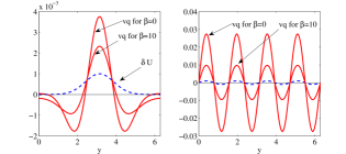
Figure 1: Mean flow acceleration resulting from a small mean flow perturbation imposed on a background of homogeneous turbulence. In the absence of a perturbation jet the vorticity flux $\overline{v^{\prime}q^{\prime}}=0$. The turbulence is distorted by the jet perturbation inducing vorticity fluxes that tend to amplify the imposed jet perturbation. In the left panel is shown a Gaussian jet perturbation together with the accelerations that it induces for $\beta=0,10$. The mean flow acceleration is not the same function as the $\delta U$ that was introduced. Right panel: when the $\delta U$ is sinusoidal the mean flow acceleration has the same form resulting in exponential growth that leads to the emergence of large scale jets. Calculations were performed in a doubly periodic square beta plane box of length $2\pi$. The coefficient of linear damping is $r=0.1$.

Consider a barotropic midlatitude beta-plane model for the dynamics of jet formation and maintenance in the Earth’s upper troposphere or in Jupiter’s atmosphere at cloud level. For simplicity assume a doubly periodic channel with $x$ and $y$ Cartesian coordinates along the zonal and the meridional direction respectively. The nondivergent zonal and meridional velocity fields are expressed in terms of a streamfunction, $\psi$, as $u=-\partial_{y}\psi$ and $v=\partial_{x}\psi$. The planetary vorticity is $2\Omega+\beta y$, with $\Omega$ the planetary rotation rate and $\beta$ the planetary vorticity gradient evaluated at the latitude of the midpoint of the channel. The relative vorticity is $q=\Delta\psi$ where $\Delta\equiv\partial^{2}_{xx}+\partial^{2}_{yy}$ is the Laplacian. The NL dynamics of this system is governed by the barotropic vorticity equation:

$$\partial_{t}q+u\,\partial_{x}q+v\,\partial_{y}q+\beta v={\cal{D}}+\sqrt{\epsilon}\,{f}~{}.$$ (22)

The term $\cal{D}$ represents linear dissipation with the zonal component of the flow (corresponding to zonal wavenumber $k=0$) dissipated at the rate $r_{m}$ while the non-zonal components are dissipated at rate $r>r_{m}$ (cf. Constantinou et al. (2014a)). This dissipation specification allows use of Rayleigh damping while still modeling the physical effect of smaller damping rate at the large jet scale than at the much smaller perturbation scale. Periodic boundary conditions are imposed in $x$ and $y$ with periodicity $2\pi L$. Distances are nondimensionalized by $L=5000\;\textrm{km}$ and time by $T=L/U$, where $U=40\;\textrm{m\,s}^{-1}$, so that the time unit is $T=1.5\;\textrm{day}$ and $\beta=10$ corresponds to a midlatitude value. Turbulence is maintained by stochastic forcing with spatial and temporal structure, ${f}$, and variance $\epsilon$.

Choosing as the averaging operator the zonal mean, i.e. $\overline{\phi}(y,t)=\int_{0}^{2\pi}\phi(x,y,t)\,dx/2\pi$ and decomposing the fields in zonal mean components and perturbations we obtain the discretized barotropic QL system:

$$\frac{dU}{dt} =\overline{v^{\prime}q^{\prime}}-r_{m}\,U~{},$$ (23a)

$$\frac{dq_{k}}{dt} =\bm{\mathsf{A}}_{k}({U})q_{k}+\sqrt{\epsilon}\,\bm{\mathsf{F}}_{k}dB_{tk}~{},$$ (23b)

where ${U}$ is the mean flow state and the subscript $k=1,\dots,N_{k}$, in (27b) indicates the zonal wavenumber and $q_{k}$ the Fourier coefficient of the perturbation vorticity that has been expanded as $q^{\prime}=\Re\left(\sum_{k=1}^{N_{k}}q_{k}e^{\mathrm{i}kx}\right)$. The $N_{k}$ wave numbers include only the zonal wavenumbers that are excited by the stochastic forcing because the $k\neq 0$ Fourier components do not directly interact in (27b) and therefore the perturbation response is limited to the wavenumbers directly excited by the stochastic forcing. The linear operator of the perturbation dynamics (27b) is given by:

$$\bm{\mathsf{A}}_{k}({U}) =-\mathrm{i}kU-\mathrm{i}k(\beta-D^{2}U)\Delta_{k}^{-1}-r~{},$$ (24)

with $\Delta_{k}=D^{2}-k^{2}$, $\Delta_{k}^{-1}$ its inverse, and $D^{2}=\partial_{yy}$. The continuous operators are discretized and approximated by matrices. The perturbation velocity appearing in (27a) is given by $v^{\prime}=\Re\left(\sum_{k=1}^{N_{k}}\mathrm{i}k\Delta_{k}^{-1}q_{k}e^{\mathrm{i}kx}\right)$, and the meridional vorticity flux accelerating the mean flow is:

$$\overline{v^{\prime}q^{\prime}}=\sum_{k=1}^{N_{k}}\frac{k}{2}{\rm diag}\left[\Im\left(\Delta_{k}^{-1}\bm{\mathsf{C}}_{k}\right)\right]~{},$$ (25)

with $\Im$ denoting the imaginary part, $\bm{\mathsf{C}}_{k}=q_{k}q_{k}^{\dagger}$ the single ensemble member covariance, $\dagger$ the Hermitian transpose, and $\rm diag$ the diagonal elements of a matrix. The forcing structure is chosen to be non-isotropic with matrix elements:

$${F}_{kij} =c_{k}\left[e^{-(y_{i}-y_{j})^{2}/(2s^{2})}+e^{-(y_{i}-2\pi-y_{j})^{2}/(2s^{2})}+\right.$$

$$\qquad\qquad\qquad+\left.e^{-(y_{i}+2\pi-y_{j})^{2}/(2s^{2})}\right],$$ (26)

with $s=0.2/\sqrt{2}$ and the normalization constants chosen so that energy is injected at each zonal wavenumber $k$ at unit rate. The delta correlation in time of the excitation ensures that this energy injection rate is the same in the QL and NL simulations and is independent of the state of the system. This forcing is chosen to model forcing of the barotropic jet in the upper atmosphere by baroclinic instability. For more details cf. Constantinou et al. (2014a).

Choosing as the averaging operator the zonal mean, i.e. $\overline{\phi}(y,t)=\int_{0}^{2\pi}\phi(x,y,t)\,dx/2\pi$ and decomposing the fields in zonal mean components and perturbations we obtain the discretized barotropic QL system:

$$\frac{dU}{dt} =\overline{v^{\prime}q^{\prime}}-r_{m}\,U~{},$$ (27a)

$$\frac{dq_{k}}{dt} =\bm{\mathsf{A}}_{k}({U})q_{k}+\sqrt{\epsilon}\,\bm{\mathsf{F}}_{k}dB_{tk}~{},$$ (27b)

where ${U}$ is the mean flow state and the subscript $k=1,\dots,N_{k}$, in (27b) indicates the zonal wavenumber and $q_{k}$ the Fourier coefficient of the perturbation vorticity that has been expanded as $q^{\prime}=\Re\left(\sum_{k=1}^{N_{k}}q_{k}e^{\mathrm{i}kx}\right)$. The $N_{k}$ wave numbers include only the zonal wavenumbers that are excited by the stochastic forcing because the $k\neq 0$ Fourier components do not directly interact in (27b) and therefore the perturbation response is limited to the wavenumbers directly excited by the stochastic forcing. The linear operator of the perturbation dynamics (27b) is given by:

$$\bm{\mathsf{A}}_{k}({U}) =-\mathrm{i}kU-\mathrm{i}k(\beta-D^{2}U)\Delta_{k}^{-1}-r~{},$$ (28)

with $\Delta_{k}=D^{2}-k^{2}$, $\Delta_{k}^{-1}$ its inverse, and $D^{2}=\partial_{yy}$. The continuous operators are discretized and approximated by matrices. The perturbation velocity appearing in (27a) is given by $v^{\prime}=\Re\left(\sum_{k=1}^{N_{k}}\mathrm{i}k\Delta_{k}^{-1}q_{k}e^{\mathrm{i}kx}\right)$, and the meridional vorticity flux accelerating the mean flow is:

$$\overline{v^{\prime}q^{\prime}}=\sum_{k=1}^{N_{k}}\frac{k}{2}{\rm diag}\left[\Im\left(\Delta_{k}^{-1}\bm{\mathsf{C}}_{k}\right)\right]~{},$$ (29)

with $\Im$ denoting the imaginary part, $\bm{\mathsf{C}}_{k}=q_{k}q_{k}^{\dagger}$ the single ensemble member covariance, $\dagger$ the Hermitian transpose, and $\rm diag$ the diagonal elements of a matrix. The forcing structure is chosen to be non-isotropic with matrix elements:

$${F}_{kij} =c_{k}\left[e^{-(y_{i}-y_{j})^{2}/(2s^{2})}+e^{-(y_{i}-2\pi-y_{j})^{2}/(2s^{2})}+\right.$$

$$\qquad\qquad\qquad+\left.e^{-(y_{i}+2\pi-y_{j})^{2}/(2s^{2})}\right],$$ (30)

with $s=0.2/\sqrt{2}$ and the normalization constants chosen so that energy is injected at each zonal wavenumber $k$ at unit rate. The delta correlation in time of the excitation ensures that this energy injection rate is the same in the QL and NL simulations and is independent of the state of the system. This forcing is chosen to model forcing of the barotropic jet in the upper atmosphere by baroclinic instability. For more details cf. Constantinou et al. (2014a).

The barotropic S3T system is:

$$\frac{dU}{dt} =\sum_{k=1}^{N_{k}}-\frac{k}{2}\Im\left({\rm diag}\left(\Delta_{k}^{-1}\bm{\mathsf{C}}_{k}\right)\right)-r_{m}U~{},$$ (31a)

$$\frac{d\bm{\mathsf{C}}_{k}}{dt} =\bm{\mathsf{A}}_{k}({U})\bm{\mathsf{C}}_{k}+\bm{\mathsf{C}}_{k}\bm{\mathsf{A}}_{k}^{\dagger}({U})+\epsilon\,\bm{\mathsf{Q}}_{k}~{},$$ (31b)

with $\bm{\mathsf{C}}_{k}=\left<q_{k}q_{k}^{\dagger}\right>$ and $\bm{\mathsf{Q}}_{k}=\bm{\mathsf{F}}_{k}\bm{\mathsf{F}}_{k}^{\dagger}$. The imaginary part in (31a) requires that we add to the system an equation for the conjugate of the covariance. This is necessary for treating the S3T equations as a dynamical system and for analyzing the stability of S3T equilibria. Alternatively we can treat the real and imaginary part of the perturbation covariance as separate variables to obtain a real S3T dynamical system as in (16).

Under the assumption that the stochastic forcing in the periodic channel is homogeneous  (31a) and (31b) admit the homogeneous equilibrium

$${U}^{e}=0~{}~{}~{}~{},~{}~{}~{}\bm{\mathsf{C}}^{e}_{k}=\frac{\epsilon}{2r}{\bm{\mathsf{Q}}_{k}}~{},$$ (32)

as shown in Appendix A. The assumption of homogeneity of the excitation is crucial for obtaining a covariance (32) and associated turbulent equilibrium with no flow, which requires that the excitation does not lead to a momentum flux convergence. If the excitation were confined to a latitude band, the homogeneous state could not be an S3T equilibrium. In that case, Rossby waves that originate from the region of excitation would dissipate in the far-field producing momentum flux convergence into the excitation region and acceleration of the mean flow there. The analysis that follows assumes that the forcing is homogeneous so that the homogeneous state (32) is an S3T equilibrium for all parameter values. The question is whether this homogeneous equilibrium is S3T stable. If it becomes S3T unstable at certain parameter values this would be an example of a flow that is hydrodynamically stable but S3T unstable.

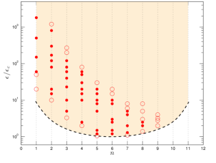
Figure 2: S3T stability diagram showing the predicted zonal flow equilibria as a function of the number of jets, $n$, and the marginal fractional amplitude of excitation $\epsilon/\epsilon_{c}$ in the doubly periodic channel (dashed curve). The amplitude, $\epsilon_{c}$, is the minimal excitation amplitude, obtained from S3T stability analysis, that renders the homogeneous state unstable. For parameter values below the dashed curve the homogeneous state is S3T stable and no jets are predicted to emerge. Above the dashed curve the flow is S3T unstable and new statistical steady states emerge characterized by the number of finite amplitude jets across the channel, $n$. S3T stable finite amplitude equilibrium jets are indicated with a full circle. Note that for given excitation amplitude there exist multiple S3T stable equilibria characterized by different numbers of jets. Unstable S3T equilibria determined with Newton iterations are indicated with open circles. Near the curve of marginal stability the S3T unstable modes other than the most unstable one at wavenumber $6$ do not continue to stable finite amplitude structures with the same wavenumber as the instability. This can be understood as a manifestation of the universal Eckhaus instability as discussed in section 5.2.4 (Parker and Krommes 2015) and in Parker and Krommes (2013). As the excitation amplitude increases jet bifurcations occur resulting in the successive establishment of stable S3T equilibria with smaller $n$. Zonal wavenumbers $k=1,\dots,14$ are forced, $\beta=10$, $r=0.1$, $r_{m}=0.01$. (Adapted from Constantinou (2015).)

a Formation and structural stability of beta-plane jets

To motivate our intuition for jet formation by cooperative interaction across spatial scales in beta-plane turbulence consider an infinitesimal perturbation of the homogeneous turbulence in the form of a small amplitude jet, $\delta{U}$, as for example the one shown in Fig. 1a, and calculate the vorticity fluxes induced by this perturbation mean flow assuming that the turbulence adjusts to $\delta{U}$ so that it satisfies the equilibrium form of (31b) with zonal mean flow perturbation $\delta U$. The modification produced in the turbulence field by this mean flow perturbation produces the steady state covariance satisfying the Lyapunov equation:

$$\bm{\mathsf{A}}_{k}(\delta{U})\bm{\mathsf{C}}_{k}+\bm{\mathsf{C}}_{k}\bm{\mathsf{A}}_{k}^{\dagger}(\delta{U})=-\epsilon\bm{\mathsf{Q}}_{k}~{},$$ (33)

for $k=1,\dots,N_{k}$. By solving (33) we find that introducing the infinitesimal jet $\delta{U}$ breaks the homogeneity of the turbulence resulting in an ensemble mean acceleration which can be calculated from (29). This induced acceleration, which is shown in Fig. 1a, is upgradient and tends to reinforce the mean flow perturbation that induced it, and this occurs even in the absence of $\beta$ (it vanishes for $\beta=0$ only if the forcing covariance is isotropic). Repeated experimentation shows that this positive feedback occurs for any mean flow perturbation under any broadband excitation (isotropic or non-isotropic) as long as there is power at sufficiently high zonal wavenumbers. This universal property of reinforcement of preexisting mean flow perturbations, revealed through S3T analysis, underlies the ubiquitous phenomenon of emergence of large scale structure in turbulent flows and explains why homogeneous equilibrium states are unstable to jet perturbations. It is clear that the acceleration induced by the test perturbation $\delta U$ shown in Fig. 1 is not identical to $\delta U$ and therefore is not an eigenfunction but if there exists a mean flow perturbation that induces accelerations with the same form as the imposed mean flow perturbation then this perturbation would be an eigenfunction of the S3T stability equations and it would grow or decay exponentially without change of form. S3T provides the framework for determining systematically the full spectrum of such eigenfunctions enabling full description of the evolution of a perturbation of small amplitude near an S3T equilibrium state. In fact, homogeneity in $y$ of the mean state assures that the mean flow component of the eigenfunctions of the S3T equilibrium (32) are harmonic so that modulo phase $\delta U_{n}=\sin(ny)$, where $n$ indicates the number of jets associated with this eigenfunction. In Fig. 1b is shown a verification that a single harmonic induces mean flow acceleration of the same form and is therefore an eigenfunction of the S3T stability equations (18).

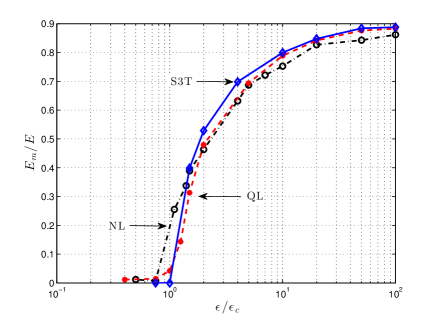
Figure 3: The ratio of the energy of the zonal mean flow, $E_{m}$, to the total energy $E$, in S3T (solid and diamonds), QL (dashed and dots), and NL (dash-dot and circles) as a function of forcing amplitude $\epsilon/\epsilon_{c}$. S3T predicts that the homogeneous flow becomes unstable at $\epsilon/\epsilon_{c}=1$ with a symmetry breaking bifurcation giving rise to finite amplitude zonal jets. This prediction of S3T is reflected accurately in the sample integrations of both QL and NL. The agreement between NL and S3T reveals that zonal jet formation is a bifurcation phenomenon and the fact that S3T predicts both the inception of the instability and the finite equilibration of the emergent flows demonstrates that the essential dynamics of the formation and nonlinear equilibration is captured by QL/S3T. Other parameters as in Fig. 2. (Adapted from Constantinou et al. (2014a).)

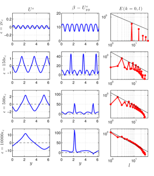
Figure 4: Left: The equilibrium mean flow ${U}^{e}$ for excitation amplitudes $\epsilon/\epsilon_{c}=2,8,150,500,10^{4}$. Center: the corresponding mean vorticity gradient $\beta-{U}_{yy}^{e}$. Right: The energy spectrum of the zonal mean flow. For the highly supercritical jets the energy spectrum approaches the approximate $l^{-5}$ dependence on meridional wavenumber $l$ found in NL simulations. We argue that in the inviscid limit this slope should approach $l^{-4}$ as the prograde jet becomes increasingly sharp. Other parameters as in Fig. 2. (Adapted from Constantinou (2015).)

Consider the stability of the homogeneous equilibrium state (32) as a function of the excitation amplitude $\epsilon$. For $\epsilon=0$ the equilibrium $U^{e}=0$ and $\bm{\mathsf{C}}_{k}^{e}=0$ is S3T stable. For $\epsilon>0$ the universal process of reinforcement of an imposed jet occurs and therefore if $r_{m}=0$ the homogeneous S3T equilibrium would immediately become unstable. For $r_{m}>0$, instability occurs for $\epsilon>\epsilon_{c}$, where $\epsilon_{c}$ is the forcing amplitude that renders the S3T stability equation neutrally stable. The normalized critical forcing amplitude for the S3T eigenfunctions with meridional wavenumber $n=1,\dots,11$ is shown in Fig. 2. S3T predicts that for these parameters the maximum S3T instability occurs for mean flow perturbations $\delta U=\sin(ny)$ with $n=6$ and thus S3T predicts that the breakdown of the homogeneous state occurs with the emergence of 6 jets in this channel.

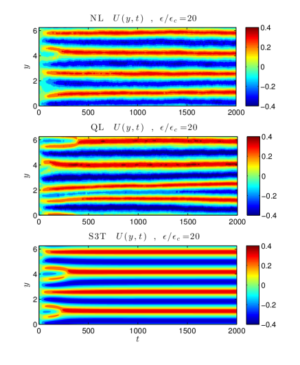
Figure 5: Hovmöller diagrams of jet emergence in NL, QL and S3T simulations for excitation $\epsilon/\epsilon_{c}=20$ as in Fig. 3. Shown for the NL, QL and S3T simulations are $U(y,t)$. In all simulations the jet structure that first emerges is the $n=6$ maximally growing jet structure predicted by S3T stability analysis. After a series of mergers S3T is attracted to a statistical steady state with a $n=4$ jet. The whole process of jet mergers and S3T equilibration is accurately reflected in the QL and NL simulations. This figure shows that S3T predicts the structure, growth and equilibration of strongly forced jets in both the QL and NL simulations. Other parameters as in Fig. 2.

b Structure of jets in beta-plane turbulence

For parameter values exceeding those required for inception of the S3T instability the S3T attractor comprises statistical steady states with finite amplitude jets that can be characterized by their zonal mean flow index $E_{m}/E$, where $E_{m}$ is the kinetic energy density of the mean flow and $E$ to the total kinetic energy density of the flow, as in Srinivasan and Young (2012). A plot of $E_{m}/E$ as a function of forcing amplitude as predicted by S3T and as observed in QL and NL, is shown in Fig. 3 and the corresponding meridional structures of the jet equilibria for various parameter values are shown in Fig. 4. Jets corresponding to S3T equilibria must be hydrodynamically stable, which generally requires with the mean vorticity gradient $\beta-{U}^{e}_{yy}$ of the equilibrium jets not change sign as the coefficient of the linear damping becomes vanishingly small. Consistent with being constrained by this criterion, the equilibrated jets at high supercriticality shown in Fig. 4 assume the characteristic shape of sharply pointed prograde jets, with very large negative curvature, and smooth retrograde jets which satisfy $\beta\approx{U}^{e}_{yy}$. This consideration leads to the prediction that the mean spacing of the jets at high supercriticality is approximately given by $\sqrt{|U_{\min}|/\beta}$, with $U_{\min}$ the peak retrograde mean zonal velocity. At low supercriticality jet amplitude is too low for instability to be a factor in constraining jet structure with typical planetary values of $\beta$ and the jets equilibrate with nearly the structure of their associated eigenmode, as discussed in Farrell and Ioannou (2007). While the spacing of highly supercritical jets could be interpreted as corresponding to Rhines scaling, the mechanism that produces this scaling is associated with the modal stability boundary of the finite amplitude jet and is unrelated to the traditional interpretation of Rhines’ scaling in terms of arrest of turbulent cascades.

S3T also predicts that the Fourier energy spectrum of the mean zonal flow of the highly supercritical jets has approximate $l^{-5}$ dependence on meridional wavenumber, $l$, in accord with highly resolved nonlinear simulations (Sukariansky et al. 2002; Danilov and Gurarie 2004; Galperin et al. 2004) as well as observations (Galperin et al. 2014). The finite amplitude jets obtained as fixed point equilibria in S3T are characterized by near discontinuity in the shear at the maxima of the prograde jets. This discontinuity would be consistent with a zonal energy spectrum proportional to $l^{-4}$. However, this discontinuity can not materialize in the presence of diffusion and it is smoothed resulting in the approximate $l^{-5}$ dependence seen in simulations. Note that S3T not only predicts the energy spectrum of the zonal jets but in addition the structure and therefore the phase of the spectral components. The occurrence of this power law is theoretically anticipated by S3T because the upgradient fluxes act as a negative diffusion on the mean flow and as a result tend to produce constant shear equilibria at each flank of the jet resulting in the near discontinuity observed in the derivative of the prograde jet (Farrell and Ioannou 2007).

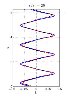
Figure 6: The S3T equilibrium jet (solid-blue) for $\epsilon/\epsilon_{c}=20$, and its reflection in a NL simulation (dash-dot-black) and a QL simulation (dashed - red). The jets in NL and QL undergo small fluctuations as is evident in Fig. 5 so shown is the average jet structure over 500 units of time. This figure shows that S3T predicts the structure of strongly forced jets in both the QL and NL simulations. Other parameters as in Fig. 2.

c Comments on statistical equilibria in beta-plane turbulence

turbulence are predictions of S3T that could not result from analysis within the NL and QL systems as in both NL and QL turbulent states with stable statistics do not exist as fixed point equilibria so that a meaningful structural stability analysis of statistically stable equilibria states can not be performed. However, as revealed in Fig. 3, Fig. 5 and Fig. 6, reflections of the bifurcation structure and of the finite amplitude equilibria predicted by the S3T closure dynamics can be clearly seen both in QL and NL sample simulations. The reflection in NL of the bifurcation structure predicted by S3T for $\epsilon\approx\epsilon_{c}$ is particularly significant because it shows that the S3T perturbation instability faithfully reflects the physics underlying jet formation in turbulence even as it manifests for infinitesimal mean flows. For a more detailed discussion cf. Constantinou et al. (2014a).

7 Applying S3T to study SSD equilibria in baroclinic turbulence

A 2D barotropic fluid lacks a source term to maintain vorticity against dissipation and therefore it cannot self-sustain turbulence. Perhaps the simplest model that self-sustains turbulence is the baroclinic two-layer model, which is essentially two barotropic fluids sharing a horizontal boundary. We use this model to study the statistical state dynamics of baroclinic turbulence. The perturbation-perturbation nonlinearity has been shown to be accurately parameterized in S3T studies of baroclinic turbulence by using a state independent stochastic excitation as a closure (DelSole and Farrell 1996; DelSole and Hou 1999; DelSole 2004b). The dynamics of baroclinic turbulence has also been studied using S3T with a state dependent closure with similar results (Farrell and Ioannou 2009c).

Consider a two layer fluid with quasi-geostrophic dynamics. The layers are of equal depth $h/2$ and bounded by horizontal rigid walls at the bottom and the top. Variables in the top layer are denoted with subscript 1, and in the bottom layer with subscript 2. The top layer density is $\rho_{1}$ and the bottom $\rho_{2}$ with $\rho_{2}>\rho_{1}$ and the potential vorticity of the layer is $q_{i}=\Delta\psi_{i}+\beta y+(-1)^{i}2\lambda^{2}(\psi_{1}-\psi_{2})/2$ ($i=1,2$), with $\lambda^{2}=2f_{0}^{2}/(g^{\prime}h)$, where $g^{\prime}=g(\varrho_{2}-\varrho_{1})/\varrho_{1}$ is the reduced gravity, and $f_{0}$ the Coriolis parameter so that, in terms of the Rossby radius of deformation $L_{d}=\sqrt{g^{\prime}h}/f_{0}$, $\lambda=\sqrt{2}/L_{d}$. The flow is relaxed to a constant temperature gradient in the meridional direction ($y$) which through the thermal wind relation induces, in the absence of turbulence and at equilibrium, a meridionally independent mean shear $H_{T}$ in the zonal ($x$) mean velocity. This shear is taken without loss of generality to result from relaxation to zero velocity in the bottom layer ($2$) and a constant mean flow with stream function $-H_{T}y$ in the top layer (1). Relaxation to this velocity structure is induced by Newtonian cooling and the bottom layer is dissipated by Ekman damping. The quasi-geostrophic dynamics governing this system is given by:

$$\partial_{t}q_{1}+J(\psi_{1},q_{1}) =\;\;\,2\lambda^{2}r_{T}\frac{\psi_{1}-\psi_{2}+H_{T}y}{2}\ ,$$ (34a)

$$\partial_{t}q_{2}+J(\psi_{2},q_{2}) =-2\lambda^{2}r_{T}\frac{\psi_{1}-\psi_{2}+H_{T}y}{2}-r\Delta\psi_{2}\ ,$$ (34b)

in which the advection of potential vorticity is expressed using the Jacobian $J(\psi,q)=\partial_{x}\psi\partial_{y}q-\partial_{y}\psi\partial_{x}q$, $r_{T}$ is the coefficient of the Newtonian cooling and $r$ is the coefficient of Ekman damping. Equations (34) have been made non-dimensional with length scale $L_{d}=1000~{}\rm km$ and time scale $1~{}\rm day$. With this scaling $\lambda=\sqrt{2}$, the velocity unit is $11.5~{}\rm ms^{-1}$ and a typical midlatitude value of $\beta=1.4$. These equations can be expressed alternatively in terms of the barotropic $\psi=(\psi_{1}+\psi_{2})/2$ and baroclinic $\theta=(\psi_{1}-\psi_{2})/2$ streamfunctions as:

$$\partial_{t}\Delta\psi +J(\psi,\Delta\psi)+J(\theta,\Delta\theta)+\beta\psi_{x}=-\frac{r}{2}\Delta(\psi-\theta)$$ (35a)

$$\partial_{t}\Delta_{\lambda}\theta +J(\psi,\Delta_{\lambda}\theta)+J(\theta,\Delta\psi)+\beta\theta_{x}=$$

$$\qquad=\frac{r}{2}\Delta(\psi-\theta)+2\lambda^{2}r_{T}\left(\theta+\frac{H_{T}}{2}y\right)$$ (35b)

where $\Delta_{\lambda}\equiv\Delta-2\lambda^{2}$.

The barotropic and baroclinic streamfunctions are decomposed into a zonal mean (denoted with capitals) and deviations from the zonal mean (referred to as perturbations) as:

$$\psi=\Psi+\psi^{\prime}~{}~{}~{}\ ,~{}~{}~{}~{}~{}\theta=\Theta+\theta^{\prime}\ ,$$ (36)

and denote with $U=-\partial_{y}\Psi$ the barotropic zonal mean flow and with $H=-\partial_{y}\Theta$ the baroclinic zonal mean flow. With this decomposition we obtain the equations for the evolution of the barotropic and baroclinic zonal mean flows:

$$\partial_{t}U =\overline{\psi_{x}^{\prime}\psi_{yy}^{\prime}+\theta_{x}^{\prime}\theta_{yy}^{\prime}}-\frac{r}{2}(U-H)-r_{m}U+\nu D^{2}U$$ (37a)

$$\partial_{t}D^{2}_{\lambda}H =D^{2}\left(\overline{\psi_{x}^{\prime}D^{2}_{\lambda}\theta^{\prime}+\theta_{x}^{\prime}\psi_{yy}^{\prime}}\right)+\frac{r}{2}D^{2}(U-H)+$$

$$~{}~{}~{}~{}~{}~{}~{}~{}~{}+2\lambda^{2}r_{T}\left(H-\frac{H_{T}}{2}\right)-r_{m}D^{2}_{\lambda}H+\nu D^{2}D^{2}H\ ,$$ (37b)

with $D^{2}\equiv\partial_{y}$, $D^{2}_{\lambda}\equiv\partial_{y}-2\lambda^{2}$, subscripts $x$ and $y$ denoting differentiation and the overline denoting zonal averaging. The corresponding barotropic and baroclinic components of the zonal mean flow deviations are $U=-\Psi_{y}$ and $H=-\Theta_{y}$. The equations for the evolution of the perturbations are:

$$\partial_{t}\Delta\psi^{\prime}+U\partial_{x}\Delta\psi^{\prime}+H\partial_{x}\Delta\theta^{\prime}+(\beta-D^{2}U)\partial_{x}\psi^{\prime}-$$

$$~{}~{}-D^{2}H\partial_{x}\theta^{\prime}=-\frac{r}{2}\Delta(\psi^{\prime}-\theta^{\prime})-r_{p}\Delta\psi^{\prime}+\nu\Delta\Delta\psi^{\prime}$$

$$\qquad\qquad\qquad\qquad-J(\psi^{\prime},\Delta\psi^{\prime})^{\prime}-J(\theta^{\prime},\Delta\theta^{\prime})^{\prime},$$ (38a)

$$\partial_{t}\Delta_{\lambda}\theta^{\prime}+H\partial_{x}\Delta\psi^{\prime}+U\partial_{x}\Delta_{\lambda}\theta^{\prime}+(\beta-D^{2}U)\partial_{x}\theta^{\prime}-$$

$$-D^{2}_{\lambda}H\partial_{x}\psi^{\prime}=\frac{r}{2}\Delta(\psi^{\prime}-\theta^{\prime})+2\lambda^{2}r_{T}\theta^{\prime}-r_{p}\Delta_{\lambda}\theta^{\prime}+$$

$$\qquad\qquad\qquad\qquad+\nu\Delta\Delta\theta^{\prime}-J(\psi^{\prime},\Delta_{\lambda}\theta^{\prime})^{\prime}-J(\theta^{\prime},\Delta\psi^{\prime})^{\prime}\ ,$$ (38b)

with the prime Jacobians denoting the perturbation-perturbation interactions,

$$J(A,B)^{\prime}=J(A,B)-\overline{J(A,B)}\ .$$ (39)

We have allowed in (37) and (38) for linear dissipation of the mean at rate $r_{m}$ and of the perturbations at rate $r_{p}$. This choice in decay rates reflects the different rates of dissipation of the mean flow and the perturbation field, which in natural flows is concentrated at smaller scales. We have also included diffusive dissipation of the velocity field with coefficient $\nu$. Equations (37) and (38) comprise the NL system that governs the two layer baroclinic flow. We impose periodic boundary conditions at the channel walls on $\Psi$, $\Theta$, $\psi^{\prime}$, $\theta^{\prime}$ as in Haidvogel and Held (1980); Panetta (1993). These boundary conditions can be verified to require that the zonally and meridionally averaged velocity at all times remains equal to that of the radiative equilibrium flow, which in turn implies that the temperature difference between the channel walls, and therefore the channel mean criticality, remains fixed.

The corresponding QL system is obtained by substituting for the perturbation-perturbation interaction a state independent and temporally delta correlated stochastic excitation together with sufficient added diffusive dissipation to obtain an approximately energy conserving closure (DelSole and Farrell 1996; DelSole and Hou 1999; DelSole 2004b). Under these assumptions the QL perturbation equations for the Fourier components of the barotropic and baroclinic streamfunction are:

$$\frac{d\psi_{k}}{dt}=\bm{\mathsf{A}}_{k}^{\psi\psi}\psi_{k}+\bm{\mathsf{A}}_{k}^{\psi\theta}\theta_{k}+\sqrt{\epsilon}\,\Delta_{k}^{-1}\bm{\mathsf{F}}_{k}\,\xi^{\psi}(t)\ ,$$ (40a)

$$\frac{d\theta_{k}}{dt}=\bm{\mathsf{A}}_{k}^{\theta\psi}\psi_{k}+\bm{\mathsf{A}}_{k}^{\theta\theta}\theta_{k}+\sqrt{\epsilon}\,\Delta_{k\lambda}^{-1}\bm{\mathsf{F}}_{k}\,\xi^{\theta}(t)\ ,$$ (40b)

in which we have assumed that the barotropic and baroclinic streamfunctions are excited respectively by $\sqrt{\epsilon}\Delta_{k}^{-1}\bm{\mathsf{F}}_{k}\xi^{\psi}$ and $\sqrt{\epsilon}\Delta_{k\lambda}^{-1}\bm{\mathsf{F}}_{k}\xi^{\theta}$. We also assume that $\xi^{\psi}$ and $\xi^{\theta}$ are independent temporally delta correlated stochastic processes of unit variance and that the perturbation fields have been expanded as $\psi^{\prime}=\Re\left(\sum_{k}\psi_{k}e^{ikx}\right)$ and $\theta^{\prime}=\Re\left(\sum_{k}\theta_{k}e^{ikx}\right)$. The operators $\bm{\mathsf{A}}_{k}$ linearized about the mean zonal flow ${\cal U}=[U,H]^{T}$ are

$$\bm{\mathsf{A}}_{k}({\cal U})~{}=~{}\left(\begin{array}[]{cc}\bm{\mathsf{A}}_{k}^{\psi\theta}&\bm{\mathsf{A}}_{k}^{\psi\theta}\\ \bm{\mathsf{A}}_{k}^{\theta\psi}&\bm{\mathsf{A}}_{k}^{\theta\theta}\\ \end{array}\right)$$ (41)

with :

$$\bm{\mathsf{A}}_{k}^{\psi\psi} =\Delta_{k}^{-1}\left[-\mathrm{i}kU\Delta_{k}-\mathrm{i}k\left(\beta-D^{2}U\right)\right]-\frac{r}{2}-r_{p}~{}+\nu\Delta_{k},$$ (42a)

$$\bm{\mathsf{A}}_{k}^{\psi\theta} =\Delta_{k}^{-1}\left[-\mathrm{i}kH\Delta_{k}+\mathrm{i}kD^{2}H\right]+\frac{r}{2}\ ,$$ (42b)

$$\bm{\mathsf{A}}_{k}^{\theta\psi} =\Delta_{k\lambda}^{-1}\left[-\mathrm{i}kH\Delta_{k}+\mathrm{i}kD^{2}_{\lambda}H+\frac{r}{2}\Delta_{k}\right]\ ,$$ (42c)

$$\bm{\mathsf{A}}_{k}^{\theta\theta} =\Delta_{k\lambda}^{-1}\left[-\mathrm{i}kU\Delta_{k\lambda}-\mathrm{i}k\left(\beta-D^{2}U\right)-\right.$$

$$\hskip 76.82234pt\left.\vphantom{\left(\beta-D^{2}U\right)}-\frac{r}{2}\Delta_{k}+2r_{T}\lambda^{2}+\nu\Delta_{k}\Delta_{k}\right]-r_{p}\ ,$$ (42d)

and $\Delta_{k}\equiv D^{2}-k^{2}$, $\Delta_{k\lambda}\equiv\Delta_{k}-2\lambda^{2}$. Continuous operators are discretized and the dynamical operators approximated by finite dimensional matrices. The states $\psi_{k}$ and $\theta_{k}$ are represented by a column vector with entries the complex value of the barotropic and baroclinic streamfunction at the collocation points in $(y)$.

The corresponding S3T system is obtained by forming from the QL equations (40) the Lyapunov equation for the evolution for the zonally averaged covariance of the perturbation field which takes the form:

$$\frac{d\bm{\mathsf{C}}_{k}}{dt}~{}=~{}\bm{\mathsf{A}}_{k}({\cal U})\,\bm{\mathsf{C}}_{k}~{}+\bm{\mathsf{C}}_{k}\,\bm{\mathsf{A}}_{k}^{\dagger}({\cal U})~{}+~{}\epsilon\bm{\mathsf{Q}}_{k}\ ,$$ (43)

with the covariance for the wavenumber $k$ zonal Fourier component defined as:

$$\bm{\mathsf{C}}_{k}~{}=~{}\left(\begin{array}[]{cc}\bm{\mathsf{C}}_{k}^{\psi\psi}&\bm{\mathsf{C}}_{k}^{\psi\theta}\\ \bm{\mathsf{C}}_{k}^{\psi\theta\dagger}&\bm{\mathsf{C}}_{k}^{\theta\theta}\\ \end{array}\right)\ ,$$ (44)

where $\bm{\mathsf{C}}_{k}^{\psi\psi}=\langle\psi_{k}\psi_{k}^{\dagger}\rangle$, $\bm{\mathsf{C}}_{k}^{\psi\theta}=\langle\psi_{k}\theta_{k}^{\dagger}\rangle$, $\bm{\mathsf{C}}_{k}^{\theta\theta}=\langle\theta_{k}\theta_{k}^{\dagger}\rangle$ with $\langle\;\bullet\;\rangle$ denoting ensemble averaging, which under the ergodic assumption is equal to the zonal average. The covariance of the stochastic excitation

$$\bm{\mathsf{Q}}_{k}~{}=~{}\left(\begin{array}[]{cc}\Delta_{k}^{-1}\bm{\mathsf{F}}_{k}\bm{\mathsf{F}}_{k}^{\dagger}\Delta_{k}^{-1\dagger}&0\\ 0&\Delta_{k\lambda}^{-1}\bm{\mathsf{F}}_{k}^{\theta}\bm{\mathsf{F}}_{k}^{\theta\dagger}\Delta_{k\lambda}^{-1\dagger}\end{array}\right)\ ,$$ (45)

has been normalized so that for each $k$ a unit of energy per unit time is injected by the excitation and therefore the amplitude of the excitation is controlled by the parameter $\epsilon$.

The S3T equations for the mean flow (37) in terms of the perturbation covariances are:

$$\frac{dU}{dt} =\sum_{k}~{}\frac{k}{2}~{}{\rm diag}\left[\Im\left(D^{2}\bm{\mathsf{C}}_{k}^{\psi\psi}+D^{2}\bm{\mathsf{C}}_{k}^{\theta\theta}\right)\right]-$$

$$~{}~{}~{}~{}~{}-\frac{{r}}{2}(U-H)-r_{m}U+\nu D^{2}U,$$ (46a)

$$\frac{dD_{\lambda}^{2}H}{dt} =D^{2}\sum_{k}\frac{k}{2}~{}{\rm diag}\left[\Im\left(D^{2}_{\lambda}\bm{\mathsf{C}}_{k}^{\psi\theta\dagger}+D^{2}\bm{\mathsf{C}}_{k}^{\psi\theta}\right)\right]+$$

$$~{}~{}~{}~{}~{}+\frac{r}{2}D^{2}(U-H)+2\lambda^{2}r_{T}\left(H-\frac{H_{T}}{2}\right)-$$

$$~{}~{}~{}~{}~{}-r_{m}D^{2}_{\lambda}H+\nu D^{2}D^{2}H\ .$$ (46b)

As is the case in the previous barotropic examples, for homogeneous forcing there also exists a meridionally and zonally homogeneous turbulent S3T equilibrium state consisting of an equilibrium zonal mean flow equal to the thermal wind balanced radiative equilibrium flow ${\cal U}^{e}=[H_{T}/2,H_{T}/2]$ corresponding to layer velocities $U_{1}^{e}=H_{T}$ and $U_{2}^{e}=0$ and a perturbation field with covariances, $\bm{\mathsf{C}}_{k}^{e}$ which satisfy the corresponding steady state Lyapunov equations (43) (for the explicit expression of the equilibrium covariance see DelSole and Farrell (1995)). However, unlike in the previous case of the barotropic beta-plane example, this homogeneous equilibrium state is realizable only for parameter values for which ${\cal U}^{e}$ is hydrodynamically (baroclinically) stable. In the absence of dissipation instability occurs for this constant flow when $H_{T}>\beta/\lambda^{2}$ or, in terms of the criticality parameter $\xi=\max(U_{1}-U_{2})\lambda^{2}/\beta$, when $\xi>1$. This dissipationless criticality parameter is customarily used despite the fact that $\xi>1$ implies instability only when the meridionally uniform flow is disipationless. In the presence of dissipation the homogeneous S3T equilibrium ${\cal U}^{e}=[H_{T}/2,H_{T}/2]$ is realizable when $\xi<\xi_{c}$, where $\xi_{c}$ is the critical value for instability for the parameters of the flow being studied. Although with $\xi<\xi_{c}$ the homogeneous equilibrium state is stable to the traditional baroclinic modal instability, it becomes S3T unstable at some critical forcing amplitude $\epsilon_{c}$. For $\epsilon>\epsilon_{c}$ the turbulent flow transitions to an inhomogeneous S3T turbulent fixed point state consisting of zonal jets and their associated perturbation field. The formation of finite amplitude equilibrium jets under homogeneous forcing in this baroclinically stable regime occurs through a bifurcation similar to that discussed previously in the example of barotropic jet formation. When $\xi>\xi_{c}$ the only homogeneous states are the (unstable) laminar equilibria with $\epsilon=0$ and $\bm{\mathsf{C}}_{k}^{e}=0$ and the flow if perturbed transitions to an inhomogeneous state, which equilibrates to an inhomogeneous statistical state with zonal jet flows.

We wish to examine the equilibria that are predicted by S3T both in the baroclinically stable and unstable regimes and compare them with the turbulent states in corresponding QL and NL simulations. We consider two example cases, one with $\xi=0$, a stable case with no temperature difference across the channel, and another with $\xi=2$ in which case the temperature gradient is being relaxed to a baroclinically unstable shear.

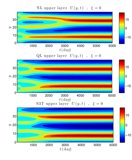
Figure 7: Hovmöller diagrams of jet emergence in NL, QL and S3T simulations under Jovian conditions with $\xi=0$. Shown for the NL, QL and S3T simulations are the flow, $U_{1}(y,t)$, in the upper layer (the flow in the lower layer is not shown as the flow is almost barotropic). After a series of mergers S3T is attracted to a statistical steady state with a $n=2$ jet. The whole process of jet mergers and S3T equilibration is accurately reflected in the QL and NL simulations. This figure shows that S3T predicts the structure, growth and equilibration of strongly forced jets in both the QL and NL simulations. The dissipation parameters in all simulations are $r=r_{T}=0$, $r_{p}=1/5$ and $r_{m}=1/2000$. The channel has $L_{x}=L_{y}=40$ and global zonal wavenumber $k=1,\dots,14$ are equally excited in energy. The total energy input by the stochastic excitation is $2.5~{}\textrm{W}\,\textrm{m}^{-2}$.

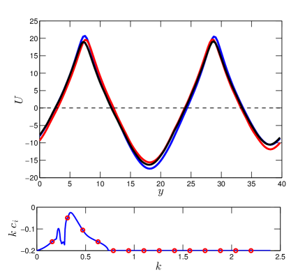
Figure 8: Comparison of the S3T equilibrium jet in the upper layer for $\xi=0$ (solid blue) with instantaneous realizations of the jet in corresponding NL (solid black) and QL (solid red) simulations. The jet is barotropic and the jet in the lower layer is not shown. The growth rate of the least damped eigenmode of the S3T equilibrium jet is shown as function of zonal wavenumber in the lower panel. The circles in this plot indicate the growth rate for each of the $14$ harmonics retained in the S3T simulation. The parameters are as in Fig. 7.

When $\xi=0$ the S3T dynamics of the two layer model is found to be essentially barotropic, similar to the examples in section 1.6, with the difference being that the deformation radius is finite. This case models the atmospheres of the outer planets which have small temperature gradients and are maintained turbulent by injection of energy by small scale convective excitation. The same stochastic excitation is applied to the S3T and QL and NL simulations by forcing the 14 gravest zonal wavenumbers, $k$, with the forcing structure $\bm{\mathsf{F}}_{k}$ chosen so that the $(i,j)$ element of the excitation is proportional to $\exp[-(y_{i}-y_{j})^{2}/(2s^{2})]$, as in (30), with $s=1/\sqrt{2}$. The total energy input by this excitation is $2.5~{}\rm Wm^{-2}$ distributed equally among the excited zonal components. The domain is a doubly periodic channel with $L_{x}=L_{y}=40$. Dissipation parameters for the NL, QL and S3T simulations are $r=r_{T}=0$, $r_{p}=1/5$ and $r_{m}=1/2000$. An example of emergence of zonal flows in this system can be seen in Fig. 7 in NL, QL and S3T and a comparison of the corresponding zonal mean flows is shown in Fig. 8. S3T predicts that for these parameters the statistics of the turbulent flow are attracted to an equilibrium with a jet and associated consistent eddy structure. The equilibrium mean flow is barotropic and barotropically stable with maximum growth rates plotted as a function of $k$ in Fig. 8. Both the NL and QL simulations reflect the predictions of S3T and the equilibrated flow has the characteristic complex structure of the $23^{\circ}$ N jet on Jupiter with the sharp prograde jets and the rounded retrograde jets (Sánchez-Lavega et al. 2008; Farrell and Ioannou 2008). The structure of the retrograde jets is not quite consistent with potential vorticity homogenization (Dritschel and McIntyre 2008), as the potential vorticity gradient of the equilibrium flow in Fig. 8 is slightly negative in limited locations of the retrograde jets which is indicative of dynamical processes beyond mixing (cf. also Fig. 3 in Farrell and Ioannou (2008)).

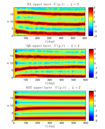
Figure 9: Hovmöller diagrams of jet emergence in NL, QL and S3T simulations under Earth-like conditions with supercritical $\xi=2$. Shown for the NL, QL and S3T simulations are the flow, $U_{1}(y,t)$, in the upper layer. The flow has substantial baroclinicity and mean flow in both layers is shown in Fig. 10. This figure shows that S3T predicts the structure, growth and equilibration of strongly forced jets in both the QL and NL simulations of self-sustained baroclinic turbulence. The dissipation parameters are $r=1/10$, $r_{T}=1/20$, $r_{p}=1/5$ and $r_{p}=1/5$ and the channel size is $L_{x}=40$ and $L_{y}=20$. In the QL and S3T simulations global zonal wavenumber $k=1,\dots,14$ are stochastically excited equally in energy with a total energy injection of $0.5~{}\textrm{W}\,\textrm{m}^{-2}$. In QL and S3T diffusive damping is included with $\nu=0.02$.

Figure 10: (a) Upper and lower layer flow in S3T (blue), QL (red) and NL (black) for supercritical equilibria with $\xi=2$. (b) Growth rate as a function of zonal wavenumber $k$ (blue curve) for the S3T equilibrated flow shown in (a) and in black the corresponding growth rate of the meridionally uniform baroclinic flow with $\xi=2$ with $r_{T}=1/15$ and $r=1/5$. With these dissipation parameters the flow becomes unstable for $\xi>\xi_{c}=0.875$. In the absence of dissipation the shortwave cut-off occurs at $k=\lambda^{2}=2$. The circles indicate the growth rate of the $k$ associated with the $14$ harmonics used in the S3T calculations. The parameters are as in Fig. 9.

Consider now the baroclinically unstable case, $\xi=2$, which represents midlatitude Earth like conditions. We again choose a doubly periodic channel with $L_{x}=40$ and $L_{y}=20$ and impose dissipation parameters $r=1/10$, $r_{T}=1/20$ and $r_{p}=r_{m}=1/5$. For these dissipation parameters the shear $H_{T}$ is baroclinically unstable (cf. a plot of the maximum growth rate of this flow as a function of zonal wavenumber is shown in Fig. 10c) and a self-sustained turbulent state develops in NL, QL and S3T. In the absence of excitation the NL simulation equilibrates to a 3 jet structure as shown in the top panel of Fig. 9 with associated jet structure shown in Fig. 10a. To obtain correspondence with the NL we parameterize the eddy interactions in the QL and S3T as in DelSole and Farrell (1996), using a state-independent stochastic forcing, with the same structure as that used for $\xi=0$. A total injection rate of $0.5~{}\rm Wm^{-2}$ in the 14 gravest zonal components and diffusion with $\nu=0.02$ bring the S3T and the QL simulations in good agreement with the NL. The agreement in the emergence of the jets and in the maintained flows are shown in Fig. 9 and Fig. 10. S3T predicts that for these parameters the statistics of the turbulent flow are attracted to an equilibrium with a jet and associated eddy structure. The mean flow is by necessity stable with growth rates shown in Fig. 10b. To avoid instability the jets become increasingly east/west asymmetric as criticality is increased with the eastward-portion equilibrating by zonal confinement (Ioannou and Lindzen 1986; James 1987; Roe and Lindzen 1996), and the westward jets equilibrating more barotropically approximately close to the Rayleigh-Kuo stability boundary while maintaining substantial baroclinicity.

A characteristic of the equilibrated jets in all cases is that while stable, they are highly non-normal and support strong transient growth. This non-normal growth is succinctly summarized in Fig. 11 (a,b) by comparison between the Frobenius norm of the resolvent of the jet perturbation dynamics

$$\left\|{\bf R}(\omega)\vphantom{R^{k}_{k}}\right\|^{2}_{F}=\sum_{k}{\rm trace}\left({\bf R}_{k}(\omega){\bf R}_{k}(\omega)^{\dagger}\right)\ ,$$ (47)

where

$${\bf R}_{k}(\omega)=-\left(\mathrm{i}\omega\bm{\mathsf{I}}+\bm{\mathsf{A}}_{k}(U^{e})\right)^{-1}\ ,$$ (48)

and its equivalent normal counterpart, with resolvent the diagonal matrix, ${\bf S}_{k}$, of the eigenvalues of $\bm{\mathsf{A}}_{k}$:

$${{\bf R}}^{\perp}_{k}(\omega)=-\left(\mathrm{i}\omega\bm{\mathsf{I}}+{\bf S}_{k}\right)^{-1}\ .$$ (49)

The square Frobenius norm of the resolvent shown as a function of frequency, $\omega$, in Fig. 11 is the ensemble mean eddy streamfunction variance, $\langle|\psi|^{2}+|\theta|^{2}\rangle$, that would be maintained by white noise forcing of this equilibrium jet. Non-normality increases the maintained streamfunction variance $\langle|\psi|^{2}+|\theta|^{2}\rangle$, over that of the equivalent normal system $\langle|\psi^{\perp}|^{2}+|\theta^{\perp}|^{2}\rangle$ and the extent of this increase is a measure of the non-normality (Farrell and Ioannou 1994; Ioannou 1995). The non-normality of the equilibria, which is associated with both baroclinic and barotropic growth processes, increases as $\xi$ increases as shown in Fig. 11.

The maintained eddy streamfunction variance, $\langle|\psi|^{2}\rangle$, in the equilibrium jet and for comparison the eddy streamfunction variance, of the equivalent normal jet system, $\langle|\psi^{\perp}|^{2}\rangle$, as a function of the criticality measure of the equilibrated flow $\xi$ is shown Fig. 12. The eddy variance maintained by the equilibrium jet increases as $\xi^{4}$ while the equivalent normal system eddy variance, $\langle|\psi^{\perp}|^{2}\rangle$, does not increase appreciably. This increase in variance with criticality is due to the increase in the non-normality of the equilibrated jet. The heat flux, which is proportional to $\langle{\theta\partial_{x}\psi}\rangle$, exhibits a $\xi^{7}$ power law behavior implying an equivalent higher order thermal diffusion. While such power law behavior is recognized to be generic to strongly turbulent equilibria (Held and Larichev 1996; Barry et al. 2002; Zurita-Gotor 2007), it lacked comprehensive explanation in the absence of the SSD-based theory for the structure of the statistical equilibrium turbulent state and its concomitant non-normality that is provided by S3T. Coexistence of very high non-normality with modal stability has been heretofore regarded as highly unlikely to occur naturally and such systems have been generally thought to result from engineering contrivance. In fact the goal of much of classical control theory is to suppress modal instability by designing stabilizing feedbacks. That this process of modal stability suppression sometimes resulted in modally stable systems that were at the same time highly vulnerable to disruption due to large transient growth of perturbation led to the more recent development of robust control theory which seeks to control transient growth associated with non-normality as well as modal stability (Doyle et al. 2009). A widely accepted argument for the necessity of engineering intervention to produce a system that is at the same time modally stable and highly non-normal follows from the observation that in the limit of increasing system non-normality, arbitrarily small perturbations to the dynamics result in modal destabilization. If the dynamics is expressed using a dynamical matrix, as we have done here, this vulnerability of the non-normal dynamics to modal destabilization finds expression in the pseudo-spectrum of the dynamical matrix (Trefethen and Embree 2005). It is remarkable that the naturally occurring feedback between the zonal mean flow and the perturbations in turbulent systems stabilizes these systems.

In summary, we have provided an explanation for the observation that adjustment to stable but highly amplifying states exhibiting power law behavior for flux/gradient relations is characteristic of strongly supercritical baroclinic turbulence. One consequence of stability coexisting with high non-normality in the Earth’s midlatitude atmosphere is the association of cyclone formation with chance occurrence in the turbulence of optimal or near optimal initial conditions (Farrell 1982, 1989; Farrell and Ioannou 1993a; DelSole 2004a). We have explained why a state of high non-normality together with marginal stability is inherent: it is because the SSD of the turbulence maintains flow stability by adjusting the system to be in the vicinity of a specific stability boundary, which is identified with the fixed point of the S3T equilibrium, while retaining the high degree of non-normality of the system. Such a state of extreme non-normality coexisting with exponential stability is an emergent consequence of the underlying SSD of baroclinic turbulence and can only result from the feedback control mechanism operating in baroclinic turbulence which has been identified by SSD analysis using S3T.

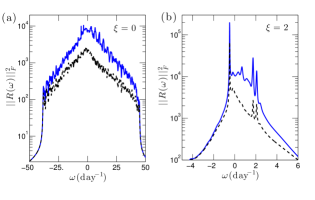
Figure 11: Panel (a): the Frobenius norm of the resolvent associated with the eddy dynamics about the equilibrium mean flow of Fig. 8 that obtains at $\xi=0$ as a function of frequency and the Frobenius norm of the resolvent of the corresponding equivalent normal eddy dynamics (dashed). Similarly in (b) for the equilibrium flow shown in Fig. 10 for $\xi=2$.

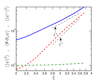
Figure 12: For the equilibrated jets shown are: the eddy barotropic streamfunction variance $\langle|\psi|^{2}\rangle$ (solid line), the eddy heat flux $\langle\theta\partial_{x}\psi\rangle$ (dashed line), and the eddy barotropic streamfunction variance maintained by the equivalent normal system $\langle|\psi^{\perp}|^{2}\rangle$ (dash-dot line) as a function of the criticality parameter $\xi$. The eddy barotropic streamfunction variance increases as $\xi^{4}$, the heat flux increases as $\xi^{7}$, while the equivalent normal variance is nearly constant. The dissipation parameters are $r=1/10$, $r_{T}=1/20$, $r_{p}=1/5$, $r_{m}=1/5$, $\nu=0$ and the channel size is $L_{x}=40$ and $L_{y}=20$. The 14 gravest zonal components are excited.

8 Application of S3T to study the SSD of wall-bounded shear flow turbulence

Consider plane Couette flow between walls with velocities $\pm U_{w}$. The streamwise direction is $x$, the wall-normal direction is $y$, and the spanwise direction is $z$. Lengths are non-dimensionalized by the channel half-width, $\delta$, and velocities by $U_{w}$, so that the Reynolds number is $R=U_{w}\delta/\nu$, with $\nu$ the coefficient of kinematic viscosity. We take for our example a doubly periodic channel of non-dimensional length $L_{x}$ in the streamwise direction and $L_{z}$ in the spanwise (note we have adopted the wall-bounded turbulence convention for the vertical coordinate which differs from the meteorological convention).

In the absence of turbulence the equilibrium solution is the laminar Couette flow with velocity components $(y,0,0)$ which has been shown to be linearly stable at all Reynolds numbers (Romanov 1973) and globally stable for $R<20.7$ (Joseph 1966). However, experiments show that plane Couette flow can be induced by a perturbation to transition to a turbulent state for Reynolds numbers exceeding $R\approx 360$ (Tillmark and Alfredsson 1992). During transition to turbulence and in the turbulent state a prominent large scale structure is observed in the flow. This structure, referred to as the roll/streak, comprises a modulation of the streamwise mean flow in the spanwise direction by regions of high and low velocity, referred to as streaks, together with a set of nearly cylindrical vortices in the wall-normal/spanwise plane, referred to as rolls. The roll circulation is such that the maximum negative wall-normal velocity is coincident with the maximum positive streamwise velocity of the streak and the maximum wall-normal velocity with the minimum streak velocity. This roll circulation serves to amplify the streak by advecting the mean shear; a mechanism referred to as lift-up. The streak is analogous to the jet that develops in barotropic and baroclinic flows and roll-streak structure arises naturally from S3T instability of the spanwise homogeneous shear turbulence. To show this we formulate the S3T dynamics for this flow and demonstrate that the S3T homogeneous turbulent equilibria become unstable with the eigenfunctions of maximum growth rate being the roll-streak structures.

Consider the vector velocity field $\vec{\it U}$ to be decomposed into a streamwise mean, with components, $(U,V,W)$, and perturbation from this mean with components $(u,v,w)$. The pressure gradient is similarly decomposed into its streamwise mean, $\nabla P$, and perturbation from this mean, $\nabla p$. All streamwise averaged quantities are denoted with capitals and the streamwise averaging operation is denoted by an overline. In these variables a unit density fluid obeys the non-divergent Navier-Stokes equations:

$${\vec{\it u}_{t}}+\vec{\it U}\cdot\nabla\vec{\it u}+\vec{\it u}\cdot\nabla\vec{\it U}+\nabla{p}-\Delta{\vec{\it u}}/R=$$

$$\hskip 20.00003pt=-(\vec{\it u}\cdot\nabla\vec{\it u}-\overline{\vec{\it u}\cdot\nabla\vec{\it u}})+\vec{\it e}\ ,$$ (50a)

$${\vec{\it U}_{t}}+\vec{\it U}\cdot\nabla\vec{\it U}+\nabla{P}-\Delta{\vec{\it U}}/R=-\overline{\vec{\it u}\cdot\nabla\vec{\it u}}\ ,$$ (50b)

$$\nabla\cdot\vec{\it U}=0~{}\ ,~{}~{}\nabla\cdot\vec{\it u}=0\ ,$$ (50c)

with boundary conditions $\vec{\it u}=0$ and $\vec{\it U}=(\pm 1,0,0)$ at $y=\pm 1$ and periodicity in $x$ and $z$.

In the perturbation equation (50a) allowance is made for specifying an explicit external perturbation forcing, $\vec{\it e}$. A stochastic parameterization is now introduced to account for both this external forcing and the perturbation-perturbation interactions, $\vec{\it u}\cdot\nabla\vec{\it u}-\overline{\vec{\it u}\cdot\nabla\vec{\it u}}$. With this parameterization, the perturbation equation becomes:

$${\vec{\it u}_{t}}+\vec{\it U}\cdot\nabla\vec{\it u}+\vec{\it u}\cdot\nabla\vec{\it U}+\nabla{p}-\Delta{\vec{\it u}}/R=\vec{\it E}\ .$$ (51)

Perturbation equation (51), coupled with the mean flow equation, (50b), form the quasi-linear (QL) form of the Navier-Stokes equations. This approximate set of equations is also referred to as the restricted nonlinear (RNL) system (Thomas et al. 2014).

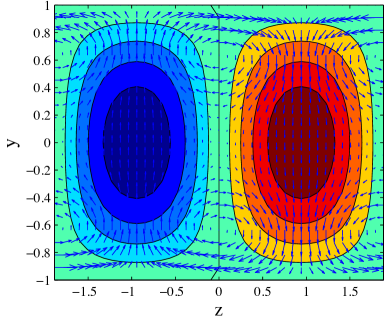
Figure 13: The rate of change of streamwise roll acceleration induced by a streak perturbation to a Couette flow that is maintained turbulent by stochastic forcing. Distortion of the turbulence by the streak perturbation induces Reynolds stresses that force roll circulations supporting the streak via the lift-up mechanism. Shown are contours of the imposed streak perturbations, $\delta U=\cos(\pi y/2)\sin(2\pi z/L_{z})$, with $\delta U>0$ in $z>0$, and vectors of the resulting rate of change of roll acceleration, $(\dot{V},\dot{W})$. The Reynolds number is $R=400$, $L_{x}=1.75\pi$ and $L_{z}=1.2\pi$. Adapted from “Dynamics of streamwise rolls and streaks in turbulent wall-bounded shear flow”, by B. F. Farrell and P. J. Ioannou, 2012, Journal of Fluid Mechanics, vol. 708, pp. 149-196. © Cambridge University Press. Reprinted with permission.

It is convenient to eliminate the pressure and express equation (51) in terms of cross-stream velocity $v$ and cross-stream vorticity, $\eta=\partial_{z}u-\partial_{x}w$. The equations then take the form:

$$\Delta v_{t}+U\Delta v_{x}+U_{zz}v_{x}+2U_{z}v_{xz}-U_{yy}v_{x}-2U_{z}w_{xy}-$$

$$\hskip 20.00003pt-2U_{yz}w_{x}-\Delta\Delta v/R=\Delta E_{v}\ ,$$ (52a)

$$\eta_{t}+U\eta_{x}-U_{z}v_{y}+U_{yz}v+U_{y}v_{z}+U_{zz}w-\Delta\eta/R=E_{\eta}\ .$$ (52b)

where $E_{v}$ and $E_{\eta}$ are the stochastic excitation in these variables (cf. Schmid and Henningson (2001)). In the perturbation equations (52), advection of perturbations by the small $V$ and $W$ components of the streamwise mean velocity has been neglected. Using nondivergence the mean flow equation (50b) can be written as:

$$U_{t} =U_{y}\Psi_{z}-U_{z}\Psi_{y}-\partial_{y}\overline{uv}-\partial_{z}\overline{uw}+\Delta_{1}U/R\ ,$$ (53a)

$$\Delta_{1}\Psi_{t} =(\partial_{yy}-\partial_{zz})(\Psi_{y}\Psi_{z}-\overline{vw})-$$

$$\hskip 20.00003pt-\partial_{yz}(\Psi_{y}^{2}-\Psi_{z}^{2}+\overline{w^{2}}-\overline{v^{2}})+\Delta_{1}\Delta_{1}\Psi/R\ .$$

In (LABEL:eq:MPSI), $\Delta_{1}\equiv\partial_{y}^{2}+\partial_{zz}^{2}$ and $V$ and $W$ have been expressed in terms of the streamfunction, $\Psi$, as $V=-\Psi_{z}$ and $W=\Psi_{y}$.

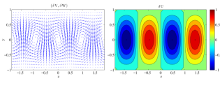
Figure 14: The most unstable streamwise roll and streak eigenfunction of the S3T system linearized about the spanwise uniform equilibrium at supercriticality $\epsilon/\epsilon_{c}=1.4$. The growth rate of this mode is $\lambda_{r}=0.014$. Shown are velocity vectors $(\delta V,\delta W)$ (left) and streamwise velocity $\delta U$ (right). The ratio of the maxima of $(\delta U,\delta V,\delta W)$ is $(1,0.06,0.03)$. Other parameters are as in Fig. 13. Adapted from “Dynamics of streamwise rolls and streaks in turbulent wall-bounded shear flow”, by B. F. Farrell and P. J. Ioannou, 2012, Journal of Fluid Mechanics, vol. 708, pp. 149-196. © Cambridge University Press. Reprinted with permission.

We next Fourier expand the perturbation fields in $x$: $v=\Re\left[\sum_{k}\hat{v}_{k}(y,z,t){e}^{\mathrm{i}kx}\right]$, $\eta=\Re\left[\sum_{k}\hat{\eta}_{k}(y,z,t){e}^{\mathrm{i}kx}\right]$, and write the equations for the evolution of the Fourier components of (52) in the matrix form

$$\frac{d\phi_{k}}{dt}=\bm{\mathsf{A}}_{k}({U})\phi_{k}+\sqrt{\epsilon}\,\bm{\mathsf{F}}_{k}dB_{tk}\ ,\$$ (54)

where the state of the system $\phi_{k}=[\hat{v}_{k},\hat{\eta}_{k}]^{T}$ comprises the values of the $\hat{v}_{k}$ and $\hat{\eta}_{k}$ on the $N=N_{y}N_{z}$ grid points of the $(y,z)$ plane and

$$\bm{\mathsf{A}}_{k}({U}) =\left(\begin{array}[]{cc}\bm{\mathsf{L}}_{OS}&\bm{\mathsf{L}}_{C_{1}}\\ \bm{\mathsf{L}}_{C_{2}}&\bm{\mathsf{L}}_{SQ}\end{array}\right)\ ,$$ (57)

with

$$\bm{\mathsf{L}}_{OS} ={\Delta}^{-1}\left[-\mathrm{i}k{U}\Delta+\mathrm{i}k({U}_{yy}-{U}_{zz})-2\mathrm{i}k{U}_{z}\partial_{z}-\vphantom{-2\mathrm{i}k({U}_{z}\partial_{yyz}^{3}+{U}_{yz}\partial_{yz}^{2})\Delta_{2}^{-1}+{\Delta\Delta}/{R}}\right.$$

$$\qquad\left.-2\mathrm{i}k({U}_{z}\partial_{yyz}^{3}+{U}_{yz}\partial_{yz}^{2})\Delta_{2}^{-1}+{\Delta\Delta}/{R}\right],$$ (58a)

$$\bm{\mathsf{L}}_{C_{1}} =2k^{2}\Delta^{-1}\left({U}_{z}\partial_{y}+{U}_{yz}\right)\Delta_{2}^{-1},$$ (58b)

$$\bm{\mathsf{L}}_{C_{2}} ={U}_{z}\partial_{y}-{U}_{y}\partial_{z}-{U}_{yz}+{U}_{zz}\partial_{yz}^{2}\Delta_{2}^{-1},$$ (58c)

$$\bm{\mathsf{L}}_{SQ} =-\mathrm{i}k{U}\Delta+\mathrm{i}k{U}_{zz}\Delta_{2}^{-1}+{\Delta}/{R}~{},$$ (58d)

being the conventionally designated Orr-Somerfeld, coupling, and Squire operators respectively. In equations (58), $\Delta^{-1}$ and $\Delta_{2}^{-1}$ are the inverses of the matrix Laplacians, $\Delta$ and $\Delta_{2}=\partial_{x}^{2}+\partial_{z}^{2}$, which are rendered invertible by enforcing the boundary conditions. The boundary conditions satisfied by the Fourier amplitudes of the perturbation fields are: periodicity in $x$ and $z$ and ${\hat{{v}\mkern 2.0mu}\mkern-2.0mu}{}_{k}=\partial_{y}{\hat{{v}\mkern 2.0mu}\mkern-2.0mu}{}_{k}={\hat{{\eta}\mkern 2.0mu}\mkern-2.0mu}{}_{k}=0$ at $y=\pm 1$.

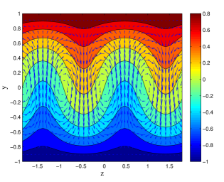
Figure 15: The finite amplitude S3T equilibrium streamwise roll and streak resulting from the equilibration of the eigenmode shown in Fig. 14 at supercriticality $\epsilon/\epsilon_{c}=1.4$. Shown are the streamwise averaged streamwise flow, $U(y,z)$, (contours) and the streamwise averaged velocities, $(V,W)$ (vectors). The maxima of the fields $(U,V,W)$ are $(0.26,0.02,0.009)$. Adapted from “Dynamics of streamwise rolls and streaks in turbulent wall-bounded shear flow”, by B. F. Farrell and P. J. Ioannou, 2012, Journal of Fluid Mechanics, vol. 708, pp. 149-196. © Cambridge University Press. Reprinted with permission.

The ensemble average perturbation covariance, $\bm{\mathsf{C}}_{k}=\langle\phi_{k}\phi_{k}^{\dagger}\rangle$, evolves according to the time-dependent Lyapunov equation:

$$\frac{{d}\bm{\mathsf{C}}_{k}}{{d}t}~{}=\bm{\mathsf{A}}_{k}({U})\,\bm{\mathsf{C}}_{k}+\bm{\mathsf{C}}_{k}\,\bm{\mathsf{A}}_{k}^{\dagger}({U})+\epsilon\,\bm{\mathsf{Q}}_{k}\ ,$$ (59)

in which: $\bm{\mathsf{Q}}_{k}=\bm{\mathsf{F}}_{k}\bm{\mathsf{F}}_{k}^{\dagger}$. If then, as previously, we make the ergodic assumption that streamwise averages are equal to ensemble averages all the quadratic fluxes that enter into the streamwise averaged flow equations (53) become linear functions of the $\bm{\mathsf{C}}_{k}$ and the mean flow evolution equations (53) can be written concisely in the form:

$$\frac{{d}{\Gamma}}{{d}t}={G}({\Gamma})+\sum_{k}{\Re}\left(\bm{\mathsf{L}}_{RS}\bm{\mathsf{C}}_{k}\right)\ ,$$ (60)

where ${\Gamma}\equiv[{U},{\Psi}]^{T}$ determines the three components of the streamwise averaged flow, the term $\sum_{k}{\Re}\left(\bm{\mathsf{L}}_{RS}\bm{\mathsf{C}}_{k}\right)$ produces by multiplying $\bm{\mathsf{C}}_{k}$ with matrix $\bm{\mathsf{L}}_{RS}$ the forcing of the mean equations by the perturbation field and $G(\Gamma)$ is the nonlinear term representing the self-advection of the streamwise averaged flow. Equations (59) and (60) comprise the S3T system for the Couette problem. The forcing covariances, $\bm{\mathsf{Q}}_{k}$, are chosen to be spanwise homogeneous. Under this assumption spanwise homogeneous S3T equilibrium states exist. For further details on the formulation see Farrell and Ioannou (2012).

The Couette flow is a laminar equilibrium of the S3T system with excitation $\epsilon=0$. For any $\epsilon$ and any spanwise homogeneous $Q_{k}$ there are always spanwise independent S3T equilibria having spanwise independent streamwise averaged flow ${U}^{e}(y)$ and ${\Psi}^{e}=0$ and spanwise homogeneous perturbation covariances $\bm{\mathsf{C}}^{e}_{k}$. These are equilibria because, consistent with the spanwise independence of both the equilibrium mean flow and the imposed excitation, $\bm{\mathsf{C}}^{e}_{k}$ is also spanwise independent and this results in ensemble mean $\overline{uw}$, $\overline{v^{2}}$ and $\overline{w^{2}}$ that are independent of $z$, and $\overline{vw}$ that identically vanishes by symmetry. Consequently, (LABEL:eq:MPSI) admits $\Psi^{e}=0$ as a solution as the ensemble mean perturbation forcing vanishes. However, the ensemble mean Reynolds stress divergence $\partial_{y}\overline{uv}$ in (53a) does not vanish and ${U}^{e}(y)$ satisfies $\Delta_{1}U^{e}/R=\partial_{y}\overline{uv}$ indicating that the presence of external excitation induces a modification to the laminar Couette profile.

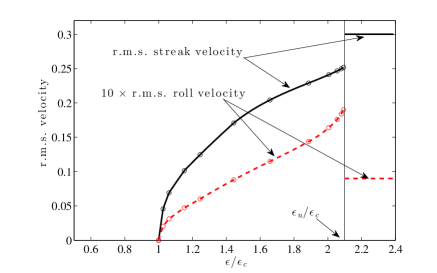
Figure 16: Typical S3T bifurcation diagram for the Couette problem. Shown are the RMS streak velocity (solid) and $10\times$ the RMS streamwise roll velocity (dashed) as a function of the perturbation forcing amplitude, $\epsilon$. For $\epsilon/\epsilon_{c}<1$, the spanwise homogeneous state is S3T stable. At $\epsilon_{c}$ the spanwise uniform equilibrium bifurcates to an equilibrium with a streamwise roll and streak. Stable streamwise roll and streak equilibria extend up to $\epsilon_{u}/\epsilon_{c}=2.1$ beyond which the streamwise roll and streak transitions to a time-dependent state which can self-sustain and the amplitudes of the roll and streak become independent of $\epsilon$. Shown for reference are the r.m.s. velocities of the streak and roll in the self-sustaining state. The Reynolds number is $R=400$, $L_{x}=1.75\pi$ and $L_{z}=1.2\pi$.

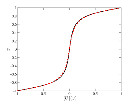
Figure 17: Comparison of the spanwise and time averaged streamwise flow, $[U](y)$, for the self-sustaining state (solid) with the mean flow obtained from a $128\times 65\times 128$ direct numerical simulation (DNS) of Couette turbulence at $R=1000$ in a doubly periodic channel in $x$ and $z$ of length $4\pi$ in each direction. The S3T self sustaining turbulent state produces on average a friction velocity based Reynolds number of $R_{\tau}=64.9$ while the DNS simulation has $R_{\tau}=66.2$. This Reynolds number indicates the turbulent production and dissipation and is defined as $R_{\tau}=u_{\tau}\delta/\nu$ with $\delta$ the channel half-width and $u_{\tau}=\sqrt{\nu\left.d[U]/dy\right|_{y=1}}$ the friction velocity. This figure demonstrates that the S3T self-sustaining state produces a streamwise averaged flow profile consistent with simulations of Couette flow turbulence. (Courtesy of V. Thomas)

In analogy with the test function probe used to elucidate the mechanism underlying jet formation in barotropic flow (cf. section a) we wish to determine the effect on the spanwise homogeneous field of turbulence of an infinitesimal spanwise-dependent mean-flow streak perturbation $\delta{U_{s}}(y,z)$ added to the equilibrium flow, $U^{e}(y)$. We are particularly interested to determine if distortion of the turbulence by the perturbation streak results in a positive feedback on the perturbation streak, $\delta{U_{s}}(y,z)$. We determine this feedback by calculating the change $\delta\bm{\mathsf{C}}_{k}$ in $\bm{\mathsf{C}}^{e}_{k}$ resulting from the streak perturbation $\delta{U_{s}}(y,z)$ as in the barotropic example. The divergence of the ensemble averaged perturbation Reynolds stresses resulting from this $\delta\bm{\mathsf{C}}_{k}$ produce a torque in the $y-z$ plane inducing a circulation, according to equation (LABEL:eq:MPSI), with streamfunction:

$$\partial_{t}{\delta\Psi}=\Delta_{1}^{-1}\left[-(\partial_{yy}-\partial_{zz})~{}\delta\,\overline{{vw}}-\partial_{yz}~{}(\delta\,\overline{{w^{2}}}-\delta\,\overline{{v^{2}}}\,)\right]\ .$$ (61)

An example streak perturbations, $\delta{U}_{s}$, together with vectors of the induced streamwise roll circulation from (61), is shown in Fig. 13. Remarkably, this streak perturbation induces a distortion of the perturbation field resulting in a streamwise roll forcing configured to amplify the imposed streak perturbation through the lift-up mechanism i.e. positive wall-normal velocity is collocated with the minimum of the streak and maximum negative wall-normal velocity is collocated with the maximum of the streak. As a result this streak perturbation, when imposed on the initially homogeneous field of turbulence, induces Reynolds stresses driving a roll circulation producing through lift-up growth of the imposed streak. This robust Reynolds stress mediated destabilizing feedback process operating on the streamwise streak and roll structure has important implications for both the transition to and the maintenance of turbulence in shear flows. We will show below that even when the streak structure is highly complex and time-dependent, as in a turbulent shear flow, the streamwise roll forcing produced by the perturbation Reynolds stresses remains collocated so as to amplify the streak. Moreover, this property of imposed streaks to induce, through modification of the perturbation field, streamwise roll forcing configured to reinforce the imposed streak provides the mechanism for a streamwise roll and streak plus turbulence cooperative instability in shear flow. This emergent instability is especially interesting because wall-bounded flows have laminar and turbulent mean velocity profiles with negative curvature and as a result do not support fast inflectional laminar flow instability as a mechanism for robustly transferring energy from the mean flow to the perturbation field as is required in order to maintain the turbulent state. While most streak perturbations organize turbulent Reynolds stresses that do not exactly amplify the streak that produced them, as is clear in the case of the streak perturbation in Fig. 13, if a streak were to organize precisely the perturbation field required for its amplification then exponential modal growth of this streak and its associated streamwise roll and perturbation fields would result.

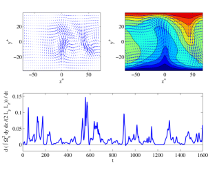
Figure 18: Streamwise roll forcing by perturbation Reynolds stresses in the self-sustaining state with $\epsilon=0$. Top left: Vectors of instantaneous cross-stream/spanwise velocity acceleration, $(\dot{V},\dot{W})$, at time $t=980$. Top right: Streamwise roll and streak structure at the same time. Lengths are measured in wall units, $y^{+}=R_{\tau}y$ and $z^{+}=R_{\tau}z$. Bottom: Time series of streamwise roll forcing as indicated by the rate of change of the average square streamwise vorticity. It is remarkable that the perturbations, in this highly time-dependent state, act to maintain the roll circulation produce, not only on average, but also at nearly every instant. Adapted from “Dynamics of streamwise rolls and streaks in turbulent wall-bounded shear flow”, by B. F. Farrell and P. J. Ioannou, 2012, Journal of Fluid Mechanics, vol. 708, pp. 149-196. © Cambridge University Press. Reprinted with permission.

We determine now the S3T stability of the spanwise homogeneous equilibrium as a function of excitation amplitude, $\epsilon$, at a fixed Reynolds number, $R$, and show that exponentially unstable streamwise roll and streak modes arise in a spanwise independent field of forced turbulence if the perturbation forcing amplitude exceeds a threshold. The spanwise independent equilibrium is stable for $\epsilon<\epsilon_{c}$. At $\epsilon_{c}$ it becomes structurally unstable, while remaining hydrodynamically stable. The most unstable eigenfunction, which is shown in Fig. 14, consists of a roll circulation with a perfectly collocated streak. When this eigenfunction is introduced into the S3T system with small amplitude, it grows at first exponentially at the rate predicted by its eigenvalue and then asymptotically equilibrates at finite amplitude. This equilibrium solution, shown in Fig. 15, is a steady, finite amplitude streamwise roll and streak. The bifurcation diagram of the S3T equilibria is shown in Fig. 16 as a function of bifurcation parameter $\epsilon$. The finite amplitude streamwise roll and streak equilibria are S3T stable for $\epsilon_{c}\leq\epsilon\leq\epsilon_{u}$.

At $\epsilon_{u}$ there is a second bifurcation in which the equilibrium becomes S3T unstable, while remaining hydrodynamically stable, and the SSD fails to equilibrate, instead transitioning directly to a time-dependent state. Remarkably, the time-dependent S3T state that emerges for $\epsilon>\epsilon_{u}$ self-sustains even when $\epsilon$ is set to $0$. This S3T self-sustaining time-dependent state produces realistic turbulence with mean turbulent profile $[U]$ shown in Fig. 17. Moreover, comparison with direct numerical simulations (DNS) verifies that this S3T turbulence is similar to Navier-Stokes turbulence despite the greatly simplified S3T dynamics underlying it (Farrell et al. 2012; Constantinou et al. 2014b; Thomas et al. 2014).

Remarkably, the S3T self-sustaining state naturally simplifies further by evolving to a minimal turbulent system in which the dynamics is supported by the interaction of the roll-streak structures with a perturbation field comprising a small number of streamwise harmonics (as few as $1$). This minimal self-sustaining turbulent system, which proceeds naturally from the S3T dynamics, reveals an underlying self-sustaining process (SSP) which can be understood with clarity. The basic ingredient of this SSP is the robust tendency for streaks to organize the perturbation field so as to produce Reynolds stresses supporting the streak, via the lift-up mechanism as illustrated in Fig. 13. Although the streak is strongly fluctuating in the self-sustaining state, the tendency of the streak to organize the perturbation field is retained as illustrated in Fig. 18 in which a snapshot of the streamwise roll and streak is shown together with the associated roll acceleration, $(\dot{V},\dot{W})$, arising from the perturbation Reynolds stresses (cf. equation (61)). The time derivative of the integral square streamwise vorticity, $d/dt(\int dy\,dz~{}\Omega_{x}^{2})$ with $\Omega_{x}=W_{y}-V_{z}$, provides a measure of the torque produced by the Reynolds stress divergences that support the roll circulation. A times series of this diagnostic is also shown in Fig. 18. It is remarkable that the perturbations, in this highly time-dependent state, produce torques that maintain the streamwise roll not only on average but at nearly every instant. As a result, in this self-sustaining state, the streamwise roll is systematically maintained by the robust organization of perturbation Reynolds stress by the time-dependent streak that was identified by SSD analysis using the S3T system, while the streak is maintained by the streamwise roll through the lift-up mechanism. Through the resulting time-dependence of the roll-streak structure the constraint on instability imposed by the absence of inflectional instability in the mean flow is bypassed and the perturbation field is maintained by parametric growth, thus completing the SSP cycle.

We conclude that the dynamics of turbulence in wall-bounded shear flow can be understood at a fundamental level by using SSD and specifically by exploiting the direct relation between wall turbulence and the highly simplified S3T turbulence. Among the results obtained is that the mechanism of turbulence in wall bounded shear flow is the same roll/streak/perturbation SSP that has been shown to maintain S3T turbulence.

9 Discussion

Although turbulence is commonly thought of as being definitional of disorder, the turbulent state in shear flow possesses an underlying order that is revealed by adopting statistical state variables to characterize the dynamics of the turbulent state. This fundamental order at the center of turbulence dynamics has remained incompletely appreciated for lack of a conceptual basis as well as of methods for analyzing the order underlying statistical states of turbulence. In this review we have described an approach to understanding emergence of order in turbulence through adopting the perspective of SSD. From this perspective order is understood to arise in turbulence due to systematic cooperative interaction between large scale structures and the field of small scale turbulence in which these structures are embedded. Motivating examples of order emergence arise from considering a field of turbulence of some kind (GFD, MHD, Navier-Stokes) into which a trial perturbation of small amplitude but large scale is introduced. When introduced, such a structure both alters the turbulence and is altered by it. Most such structures are not systematically maintained by this interaction. But suppose that we were to continue trying different large scale perturbations until we hit on a perturbation structure that affected the turbulence in just such a manner as to produce Reynolds stresses configured to amplify this structure without changing its form. Such a structure would naturally grow spontaneously out of the turbulence and would provide an explanation for the observed emergence of large scale structure in turbulent flow. This concept of coherent structure emergence through cooperative multi-scale interaction in turbulence takes analytical form through eigenanalysis of the SSD of the turbulence linearized about an equilibrium turbulent statistical state. Bifurcations occur in association with these instabilities as parameters of the problem, such as the amplitude of the turbulence excitation rate, the damping rate of the flow, or the beta parameter, are varied. Extensions of these instabilities into the nonlinear regime of the SSD reveal fixed point equilibria that predict the associated finite amplitude coherent structures e.g. the zonal jets in the case of barotropic and baroclinic turbulence in planetary atmospheres. Moreover, these finite amplitude equilibria of the nonlinear SSD have an interpretation that transcends prediction of jet structure. The statistical state of the turbulence comprises both the mean flow and the perturbations which have mutually adjusted to produce the equilibrium statistical state so that these equilibria constitute a closure of the associated turbulence dynamics. The success of SSD in predicting the statistical mean state of turbulence as S3T equilibria in the systems we have discussed argues constructively that the nonlocal in spectral space interaction between perturbations and large scale mean flows that is retained in S3T captures the physical mechanism underlying the maintenance of the turbulent state in these systems. In addition, this closure is deterministic so that the physical mechanisms producing the closure are made available for study through analysis of the SSD underlying them. A straightforward example of such an insight into closure in turbulence arises in the case of barotropic beta-plane turbulence in which the observed jet scale in strongly excited turbulence is linked mechanistically through SSD with Rayleigh’s stability criterion; SSD analysis makes the further and associated verifiable prediction of successive bifurcations to jet structure of smaller wavenumber with increase in turbulence intensity. This example shows the power of SSD to both predict and provide physical explanation for observed phenomena in turbulent flows.

Adopting the perspective of SSD also provides new conceptual insights into the dynamics of turbulence; an example of this is the concept of the dynamical trajectory of a statistical state. Consider a statistical state equilibrium consisting of a fixed point. An example might be a barotropic jet together with its supporting turbulence. This fixed point corresponds to a probability density function that is stationary in state space. But just as sample state trajectories, which are points in phase space, may converge to a fixed point or follow a time dependent path through the state space, so also statistical state trajectories may follow more or less intricate paths in phase space, taking their probability density function along with them. Interpretation of the dynamics of these statistical state trajectories provides a way to deepen understanding of the dynamic of turbulence. The successive bifurcations with increase in excitation leading to lower and lower meridional wavenumber for the equilibrium jet in the example of beta-plane turbulence mentioned above can be viewed as a trajectory of the deterministic SSD with the bifurcations arising from instability of the evolving statistical state. These trajectories and instabilities have no analytical counterpart in sample state dynamics. A familiar example of limit cycle behavior of a statistical state trajectory is provided by the QBO of the Earth’s equatorial stratosphere which exhibits nearly periodic 27 month cycles in phase space. The analytical structure of the associated bifurcation only exists in the SSD framework (Farrell and Ioannou 2003). Chaotic statistical state trajectories are also found in jet dynamics of plasma turbulence (Farrell and Ioannou 2009b). In the case of wall-bounded shear flow turbulence the statistical state trajectory is also chaotic and the time dependence of this statistical state, consisting of the streak structure and the associated perturbations it supports, which results from their cooperative interaction, is a fundamental component of the dynamical mechanism underlying the SSP maintaining the turbulence. This is because the turbulence is maintained by perturbations that result from parametric interaction with the streak, the time dependence of which is in turn maintained by interaction with the perturbations. This parametric process underlies energy transfer from the inflectionally stable forced mean flow that is required to maintain the turbulent perturbation variance in wall-bounded shear flows. This parametric growth process is intrinsically a property of the SSD and this cooperative parametric process can only be understood through analysis of the dynamics of the statistical state of the turbulence.

Viewing turbulence from the perspective of SSD has proven to be remarkably tractable and to provide a richness of analysis and concept that has already allowed progress in a number of areas and holds promise of continuing insight into the nature of turbulence.

APPENDIX A

The homogeneous equilibrium covariance

We prove that the equilibrium covariance (32) under homogeneous stochastic excitation of a channel with periodic boundary conditions produces zero mean vorticity fluxes, $\overline{v^{\prime}q^{\prime}}=0$. This is required in order for $U^{e}=0$ to be an S3T equilibrium with perturbations with covariance (32). We provide a proof that uses technical arguments that are useful for exploring the properties of discrete S3T dynamics and stability in periodic channels (cf. Bakas and Ioannou (2011)). We use the property that in the matrix formulation of S3T in a periodic channel, in which the fields have been discretized on a grid, all matrices that correspond to homogeneous continuous operators, as well as all covariances of homogeneous fields, are circulant, i.e. each row is a cyclic shift of the row above it. They are circulant because they commute with the matrix of spatial shifts on the grid lattice. Circulant matrices commute with each other and their common eigenbasis is a unitary matrix consisting of harmonics. Consequently the forcing covariance at wavenumber $k$ is analyzed in Fourier components in $y$ as $Q_{k\alpha\beta}=\sum_{l}{\hat{Q}}_{kl}e^{\mathrm{i}l(y_{\alpha}-y_{\beta})}$, with $l$ the $y$ wavenumber. Moreover, the Fourier coefficients $\hat{Q}_{kl}$ must be real and non-negative coefficients in order to assure that $Q_{k\alpha\beta}$, for each $k$, is positive definite, Hermitian and a covariance of a homogeneous field (this statement is the content of Bochner’s theorem). Because for each $k$ we have

$$\sum_{m=1}^{n}\Delta_{k\alpha m}^{-1}Q_{km\beta} =\sum_{l}\hat{Q}_{kl}\sum_{m=1}^{n}\Delta_{k\alpha m}^{-1}e^{\mathrm{i}l(y_{m}-y_{\beta})}$$

$$=-\sum_{l}\hat{Q}_{kl}\frac{e^{\mathrm{i}l(y_{\alpha}-y_{\beta})}}{k^{2}+l^{2}}$$

we obtain that the diagonal elements of $\sum_{m=1}^{n}\Delta_{k\alpha m}^{-1}C_{km\beta}^{e}$ are equal and real and therefore the vorticity flux associated with the equilibrium covariance, which is proportional to the imaginary part of the diagonal elements of this matrix, vanishes.

REFERENCES

- Ait-Chaalal et al. (2016) Ait-Chaalal, F., T. Schneider, B. Meyer, and J. B. Marston, 2016: Cumulant expansions for atmospheric flows. New. J. Phys., 18 (2), 025 019, doi:10.1088/1367-2630/18/2/025019.
- Bakas et al. (2015) Bakas, N. A., N. C. Constantinou, and P. J. Ioannou, 2015: S3T stability of the homogeneous state of barotropic beta-plane turbulence. J. Atmos. Sci., 72 (5), 1689–1712, doi:10.1175/JAS-D-14-0213.1.
- Bakas and Ioannou (2011) Bakas, N. A., and P. J. Ioannou, 2011: Structural stability theory of two-dimensional fluid flow under stochastic forcing. J. Fluid Mech., 682, 332–361, doi:10.1017/jfm.2011.228.
- Bakas and Ioannou (2013a) Bakas, N. A., and P. J. Ioannou, 2013a: Emergence of large scale structure in barotropic -plane turbulence. Phys. Rev. Lett., 110, 224 501, doi:10.1103/PhysRevLett.110.224501.
- Bakas and Ioannou (2013b) Bakas, N. A., and P. J. Ioannou, 2013b: On the mechanism underlying the spontaneous emergence of barotropic zonal jets. J. Atmos. Sci., 70 (7), 2251–2271, doi:10.1175/JAS-D-12-0102.1.
- Barry et al. (2002) Barry, L., G. C. Craig, and J. Thurbun, 2002: Poleward heat transport by the atmospheric heat engine. Nature, 415, 774–777, doi:10.1038/415774a.
- Bernstein and Farrell (2010) Bernstein, J., and B. F. Farrell, 2010: Low frequency variability in a turbulent baroclinic jet: Eddy–mean flow interactions in a two-level model. J. Atmos. Sci., 67 (2), 452–467, doi:10.1175/2009JAS3170.1.
- Brandt et al. (2004) Brandt, L., P. Schlatter, and D. S. Henningson, 2004: Transition in boundary layers subject to free-stream turbulence. J. Fluid Mech., 517, 167–198.
- Constantinou (2015) Constantinou, N. C., 2015: Formation of large-scale structures by turbulence in rotating planets. Ph.D. thesis, National and Kapodistrian University of Athens, Athens, URL http://www.didaktorika.gr/eadd/handle/10442/35501?locale=en, (also available at arXiv:1503.07644).
- Constantinou et al. (2014a) Constantinou, N. C., B. F. Farrell, and P. J. Ioannou, 2014a: Emergence and equilibration of jets in beta-plane turbulence: applications of Stochastic Structural Stability Theory. J. Atmos. Sci., 71 (5), 1818–1842, doi:10.1175/JAS-D-13-076.1.
- Constantinou et al. (2016) Constantinou, N. C., B. F. Farrell, and P. J. Ioannou, 2016: Statistical state dynamics of jet–wave coexistence in barotropic beta-plane turbulence. J. Atmos. Sci., 73 (5), 2229–2253, doi:10.1175/JAS-D-15-0288.1.
- Constantinou et al. (2014b) Constantinou, N. C., A. Lozano-Durán, M.-A. Nikolaidis, B. F. Farrell, P. J. Ioannou, and J. Jiménez, 2014b: Turbulence in the highly restricted dynamics of a closure at second order: comparison with DNS. J. Phys. Conf. Ser., 506, 012 004, doi:10.1088/1742-6596/506/1/012004.
- Danilov and Gurarie (2004) Danilov, S., and D. Gurarie, 2004: Scaling, spectra and zonal jets in beta-plane turbulence. Phys. Fluids, 16, 2592–2603, doi:10.1063/1.1752928.
- DelSole (2004a) DelSole, T., 2004a: The necessity of instantaneous optimals in stationary turbulence. J. Atmos. Sci., 61, 1086–1091.
- DelSole (2004b) DelSole, T., 2004b: Stochastic models of quasigeostrophic turbulence. Surv. Geophys., 25, 107–149, doi:10.1023/B:GEOP.0000028160.75549.0d.
- DelSole and Farrell (1995) DelSole, T., and B. F. Farrell, 1995: A stochastically excited linear system as a model for quasigeostrophic turbulence: Analytic results for one- and two-layer fluids. J. Atmos. Sci., 52, 2531–2547, doi:10.1175/1520-0469(1995)052<2531:ASELSA>2.0.CO;2.
- DelSole and Farrell (1996) DelSole, T., and B. F. Farrell, 1996: The quasi-linear equilibration of a thermally mantained stochastically excited jet in a quasigeostrophic model. J. Atmos. Sci., 53, 1781–1797, doi:10.1175/1520-0469(1996)053<1781:TQLEOA>2.0.CO;2.
- DelSole and Hou (1999) DelSole, T., and A. Y. Hou, 1999: Empirical stochastic models for the dominant climate statistics of a general circulation model. J. Atmos. Sci., 56, 3436–3456, doi:10.1175/1520-0469(1999)056<3436:ESMFTD>2.0.CO;2.
- Diamond et al. (2005) Diamond, P. H., S.-I. Itoh, K. Itoh, and T. S. Hahm, 2005: Zonal flows in plasmas – a review. Plasma Phys. Control. Fusion, 47 (5), R35–R161, doi:10.1088/0741-3335/47/5/R01.
- Doyle et al. (2009) Doyle, J. C., B. A. Francis, and T. A. R., 2009: Feedback Control Theory. Dover Publications, New York.
- Dritschel and McIntyre (2008) Dritschel, D. G., and M. E. McIntyre, 2008: Multiple jets as PV staircases: The Phillips effect and the resilience of eddy-transport barriers. J. Atmos. Sci., 65, 855–874, doi:10.1175/2007JAS2227.1.
- Farrell (1982) Farrell, B. F., 1982: The initial growth of disturbances in a baroclinic flow. J. Atmos. Sci., 39, 1663–1686, doi:10.1175/1520-0469(1982)039<1663:TIGODI>2.0.CO;2.
- Farrell (1989) Farrell, B. F., 1989: Optimal excitation of baroclinic waves. J. Atmos. Sci., 46, 1193–1206.
- Farrell et al. (2017a) Farrell, B. F., D. F. Gayme, and P. J. Ioannou, 2017a: A statistical state dynamics approach to wall-turbulence. Phil. Trans. R. Soc. A, 375 (2089), 20160 081, doi:10.1098/rsta.2016.0081.
- Farrell et al. (2012) Farrell, B. F., D. F. Gayme, P. J. Ioannou, B. K. Lieu, and M. R. Jovanovic, 2012: Dynamics of the roll and streak structure in transition and turbulence. Studying Turbulence Using Numerical Simulation Databases - XIV, Center of Turbulence Research, 43–54, (online @ ctr.stanford.edu).
- Farrell and Ioannou (1993a) Farrell, B. F., and P. J. Ioannou, 1993a: Stochastic dynamics of baroclinic waves. J. Atmos. Sci., 50, 4044–4057, doi:10.1175/1520-0469(1993)050<4044:SDOBW>2.0.CO;2.
- Farrell and Ioannou (1993b) Farrell, B. F., and P. J. Ioannou, 1993b: Stochastic forcing of the linearized Navier-Stokes equations. Phys. Fluids A, 5, 2600–2609, doi:10.1063/1.858894.
- Farrell and Ioannou (1994) Farrell, B. F., and P. J. Ioannou, 1994: Variance maintained by stochastic forcing of non-normal dynamical systems associated with linearly stable shear flows. Phys. Rev. Lett., 72, 1118–1191, doi:10.1103/PhysRevLett.72.1188.
- Farrell and Ioannou (1999) Farrell, B. F., and P. J. Ioannou, 1999: Perturbation growth and structure in time dependent flows. J. Atmos. Sci., 56, 3622–3639, doi:10.1175/1520-0469(1999)056<3622:PGASIT>2.0.CO;2.
- Farrell and Ioannou (2003) Farrell, B. F., and P. J. Ioannou, 2003: Structural stability of turbulent jets. J. Atmos. Sci., 60, 2101–2118, doi:10.1175/1520-0469(2003)060<2101:SSOTJ>2.0.CO;2.
- Farrell and Ioannou (2007) Farrell, B. F., and P. J. Ioannou, 2007: Structure and spacing of jets in barotropic turbulence. J. Atmos. Sci., 64, 3652–3665, doi:10.1175/JAS4016.1.
- Farrell and Ioannou (2008) Farrell, B. F., and P. J. Ioannou, 2008: Formation of jets by baroclinic turbulence. J. Atmos. Sci., 65, 3353–3375, doi:10.1175/2008JAS2611.1.
- Farrell and Ioannou (2009a) Farrell, B. F., and P. J. Ioannou, 2009a: Emergence of jets from turbulence in the shallow-water equations on an equatorial beta plane. J. Atmos. Sci., 66, 3197–3207, doi:10.1175/2009JAS2941.1.
- Farrell and Ioannou (2009b) Farrell, B. F., and P. J. Ioannou, 2009b: A stochastic structural stability theory model of the drift wave-zonal flow system. Phys. Plasmas, 16, 112 903, doi:10.1063/1.3258666.
- Farrell and Ioannou (2009c) Farrell, B. F., and P. J. Ioannou, 2009c: A theory of baroclinic turbulence. J. Atmos. Sci., 66, 2444–2454, doi:10.1175/2009JAS2989.1.
- Farrell and Ioannou (2012) Farrell, B. F., and P. J. Ioannou, 2012: Dynamics of streamwise rolls and streaks in turbulent wall-bounded shear flow. J. Fluid Mech., 708, 149–196, doi:10.1017/jfm.2012.300.
- Farrell and Ioannou (2017a) Farrell, B. F., and P. J. Ioannou, 2017a: Statistical state dynamics-based analysis of the physical mechanisms sustaining and regulating turbulence in Couette flow. Phys. Rev. Fluids, 2 (8), 084 608, doi:10.1103/PhysRevFluids.2.084608.
- Farrell and Ioannou (2017b) Farrell, B. F., and P. J. Ioannou, 2017b: Statistical state dynamics based theory for the formation and equilibration of Saturn’s north polar jet. Phys. Rev. Fluids, 2 (7), 073 801, doi:10.1103/PhysRevFluids.2.073801.
- Farrell et al. (2016) Farrell, B. F., P. J. Ioannou, J. Jiménez, N. C. Constantinou, A. Lozano-Durán, and M.-A. Nikolaidis, 2016: A statistical state dynamics-based study of the structure and mechanism of large-scale motions in plane Poiseuille flow. J. Fluid Mech., 809, 290–315, doi:10.1017/jfm.2016.661.
- Farrell et al. (2017b) Farrell, B. F., P. J. Ioannou, and M. A. Nikolaidis, 2017b: Instability of the roll–streak structure induced by background turbulence in pretransitional Couette flow. Phys. Rev. Fluids, 2 (3), 034 607, doi:10.1103/PhysRevFluids.2.034607.
- Fitzgerald and Farrell (2017) Fitzgerald, J. G., and B. F. Farrell, 2017: Statistical State Dynamics of vertically sheared horizontal flows in two-dimensional stratified turbulence. J. Fluid Mech., (submitted, arXiv:1612.03243).
- Frisch (1995) Frisch, U., 1995: Turbulence: The Legacy of A. N. Kolmogorov. Cambridge University Press.
- Galperin et al. (2004) Galperin, B., H. Nakano, H.-P. Huang, and S. Sukoriansky, 2004: The ubiquitous zonal jets in the atmospheres of giant planets and Earth’s oceans. Geophys. Res. Lett., 31, 13 303–13 308, doi:10.1029/2004GL019691.
- Galperin et al. (2014) Galperin, B., R. M. B. Young, S. Sukoriansky, N. Dikovskaya, P. L. Read, A. L. Lancaster, and D. Armstrong, 2014: Cassini observations reveal a regime of zonostrophic macroturbulence on Jupiter. Icarus, 229, 295–320, doi:10.1016/j.icarus.2013.08.030.
- Haidvogel and Held (1980) Haidvogel, D. B., and I. M. Held, 1980: Homogeneous quasi-geostrophic turbulence driven by a uniform temperature gradient. J. Atmos. Sci., 37, 2644–2660, doi:10.1175/1520-0469(1980)037<2644:HQGTDB>2.0.CO;2.
- Held and Larichev (1996) Held, I. M., and V. D. Larichev, 1996: A scaling theory for horizontally homogeneous, baroclinically unstable flow on a beta plane. J. Atmos. Sci., 53, 946–952, doi:10.1175/1520-0469(1996)053<0946:ASTFHH>2.0.CO;2.
- Hopf (1952) Hopf, E., 1952: Statistical hydromechanics and functional calculus. J. Ration. Mech. Anal., 1, 87–123, doi:10.1512/iumj.1952.1.51004.
- Ingersoll (1990) Ingersoll, A. P., 1990: Atmospheric dynamics of the outer planets. Science, 248, 308–315, doi:10.1126/science.248.4953.308.
- Ioannou (1995) Ioannou, P. J., 1995: Non-normality increases variance. J. Atmos. Sci., 52, 1155–1158, doi:10.1175/1520-0469(1995)052<1155:NIV>2.0.CO;2.
- Ioannou and Lindzen (1986) Ioannou, P. J., and R. S. Lindzen, 1986: Baroclinic instability in the presence of barotropic jets. J. Atmos. Sci., 43, 2999–3014, doi:10.1175/1520-0469(1986)043<2999:BIITPO>2.0.CO;2.
- James (1987) James, I. N., 1987: Suppression of baroclinic instability in horizontally sheared flows. J. Atmos. Sci., 44 (24), 3710–3720, doi:10.1175/1520-0469(1987)044<3710:SOBIIH>2.0.CO;2.
- Joseph (1966) Joseph, D. D., 1966: Nonlinear stability of the boussinesq equations by the method of energy. Arch. Rat. Mech. Anal., 22, 163–184.
- Kraichnan (1959) Kraichnan, R. H., 1959: The structure of isotropic turbulence at very high reynolds numbers. J. Fluid Mech., 5, 497–543.
- Kraichnan (1971) Kraichnan, R. H., 1971: An almost-Markovian Galilean-invariant turbulence model. J. Fluid Mech., 47, 513–524, doi:10.1017/S0022112071001204.
- Lee and Held (1991) Lee, S., and I. M. Held, 1991: Subcritical instability and hysteresis in a two-layer model. J. Atmos. Sci., 48, 1071–1077.
- Lindzen (1993) Lindzen, R. S., 1993: Baroclinic neutrality and the tropopause. J. Atmos. Sci., 50 (8), 1148–1151, doi:10.1175/1520-0469(1993)050<1148:BNATT>2.0.CO;2.
- Marston (2010) Marston, J. B., 2010: Statistics of the general circulation from cumulant expansions. Chaos, 20, 041 107, doi:10.1063/1.3490719.
- Marston (2012) Marston, J. B., 2012: Atmospheres as nonequilibrium condensed matter. Annu. Rev. Condens. Matter Phys., 3, 285–310, doi:10.1146/annurev-conmatphys-020911-125114.
- Marston et al. (2016) Marston, J. B., G. P. Chini, and S. M. Tobias, 2016: Generalized quasilinear approximation: Application to zonal jets. Phys. Rev. Lett., 116 (21), 214 501 EP –5, doi:10.1103/PhysRevLett.116.214501.
- Marston et al. (2008) Marston, J. B., E. Conover, and T. Schneider, 2008: Statistics of an unstable barotropic jet from a cumulant expansion. J. Atmos. Sci., 65 (6), 1955–1966, doi:10.1175/2007JAS2510.1.
- Øksendal (2000) Øksendal, B., 2000: Stochastic Differential Equations. Springer-Verlag, Berlin.
- Orszag (1977) Orszag, S. A., 1977: Statistical theory of turbulence. Fluid Dynamics, Les Houches 1973, R. Balian, and J. L. Peube, Eds., Gordon and Breach, New York.
- Panetta (1993) Panetta, R. L., 1993: Zonal jets in wide baroclinically unstable regions: persistence and scale selection. J. Atmos. Sci., 50, 2073–2106, doi:10.1175/1520-0469(1993)050<2073:ZJIWBU>2.0.CO;2.
- Parker and Krommes (2013) Parker, J. B., and J. A. Krommes, 2013: Zonal flow as pattern formation. Phys. Plasmas, 20, 100 703, doi:10.1063/1.4828717.
- Parker and Krommes (2014) Parker, J. B., and J. A. Krommes, 2014: Generation of zonal flows through symmetry breaking of statistical homogeneity. New J. Phys., 16 (3), 035 006, doi:10.1088/1367-2630/16/3/035006.
- Parker and Krommes (2015) Parker, J. B., and J. A. Krommes, 2015: Zonal flow as pattern formation. Zonal jets: Phenomenology, genesis, physics, B. Galperin, and P. L. Read, Eds., Cambridge University Press, chap. 5.
- Roe and Lindzen (1996) Roe, H. H., and R. S. Lindzen, 1996: Baroclinic adjustment in a two-level model with barotropic shear. J. Atmos. Sci., 53 (18), 2749–2754, doi:10.1175/1520-0469(1996)053<2749:BAIATL>2.0.CO;2.
- Romanov (1973) Romanov, V. A., 1973: Stability of plane-parallel Couette flow. Funct. Anal. Appl., 7, 137–146.
- Rose and Sulem (1978) Rose, H. A., and P.-L. Sulem, 1978: Fully developed turbulence and statistical mechanics. J. Phys. France, 39, 441–484.
- Sánchez-Lavega et al. (2008) Sánchez-Lavega, A., and Coauthors, 2008: Depth of a strong Jovian jet from a planetary-scale disturbance driven by storms. Nature, 451 (7177), 437–440, doi:10.1038/nature06533.
- Schmid and Henningson (2001) Schmid, P. J., and D. S. Henningson, 2001: Stability and Transition in Shear Flows. Springer, New York.
- Schneider and Walker (2006) Schneider, T., and C. C. Walker, 2006: Self-organization of atmospheric macroturbulence into critical states of weak nonlinear eddy-eddy interactions. J. Atmos. Sci., 63 (6), 1569–1586, doi:10.1175/JAS3699.1.
- Srinivasan and Young (2012) Srinivasan, K., and W. R. Young, 2012: Zonostrophic instability. J. Atmos. Sci., 69 (5), 1633–1656, doi:10.1175/JAS-D-11-0200.1.
- Stone and Nemet (1996) Stone, P. H., and B. Nemet, 1996: Baroclinic adjustment: A comparison between theory, observations, and methods. J. Atmos. Sci., 53, 1663–1674.
- Sukariansky et al. (2002) Sukariansky, S., B. Galperin, and N. Dikovskaya, 2002: Universal spectrum of two dimensional turbulence on rotating sphere and some basic features of atmospheric circulations on giant planets. Phys. Rev. Lett., 89, 124 501–4.
- Thomas et al. (2015) Thomas, V., B. F. Farrell, P. J. Ioannou, and D. F. Gayme, 2015: A minimal model of self-sustaining turbulence. Phys. Fluids, 27, 105 104, doi:10.1063/1.4931776.
- Thomas et al. (2014) Thomas, V., B. K. Lieu, M. R. Jovanović, B. F. Farrell, P. J. Ioannou, and D. F. Gayme, 2014: Self-sustaining turbulence in a restricted nonlinear model of plane Couette flow. Phys. Fluids, 26, 105 112, doi:10.1063/1.4898159.
- Tillmark and Alfredsson (1992) Tillmark, N., and P. H. Alfredsson, 1992: Experiments on transition in plane couette flow. J. Fluid Mech., 235, 89–92.
- Tobias et al. (2011) Tobias, S. M., K. Dagon, and J. B. Marston, 2011: Astrophysical fluid dynamics via direct numerical simulation. Astrophys. J., 727, 127, doi:10.1088/0004-637X/727/2/127.
- Trefethen and Embree (2005) Trefethen, L. N., and M. Embree, 2005: Spectra and Pseudospectra: The Behavior of Nonnormal Matrices and Operators. Princeton University Press, Princeton.
- Woillez and Bouchet (2017) Woillez, E., and F. Bouchet, 2017: Theoretical prediction of Reynolds stresses and velocity profiles for barotropic turbulent jets. EPL Europhys. Lett., 118 (5), 54 002, doi:10.1209/0295-5075/118/54002.
- Zurita-Gotor (2007) Zurita-Gotor, P., 2007: The relation between baroclinic adjustment and turbulent diffusion in the two-layer model. J. Atmos. Sci., 64, 1284–1300.