Improving approximate RPCA with a k-sparsity prior

Abstract

A process centric view of robust PCA (RPCA) allows its fast approximate implementation based on a special form of a deep neural network with weights shared across all layers. However, empirically this fast approximation to RPCA fails to find representations that are parsemonious. We resolve these bad local minima by relaxing the elementwise L1 and L2 priors and instead utilize a structure inducing k-sparsity prior. In a discriminative classification task the newly learned representations outperform these from the original approximate RPCA formulation significantly.

1 Introduction

In this work an efficient implementation of sparse coding is evaluated. Sparse coding is an optimisation problem, where it is to find a sparse representation of given data. Not only is it diffcult to find a mapping from the sparse code to the data but the search for the perfect sparse code for a single datapoint is a single extra optimisation procedure. This process is very time intensive because you need to optimize two problems one after another. The idea behind an efficient implementation of this sparse coding problem comes from sprechmann_learning_2012 gregor_learning. A gradient descent algorithm optimizing the sparse code with many iteration is transformed into a neural network with very few layers, each representing one iteration of the gradient descent algorithm. This network is then trained using the same objective function as used for creating the gradient descent iterates creating an efficient version of the initial optimisation procedure.

The Robust Principal Component Analysis (RPCA or Robust PCA)sprechmann_learning_2012 candes_robust_2011 version of such an efficient sparse coding network is evaluated. An own optimised version of this algorithm producing much sparser latent codes is presented and evaluated.

2 Robust PCA

The motivation behind Robust PCA is the decomposition of a large matrix into a low rank matrix and a sparse matrix candes_robust_2011. The sparse matrix is also called outlier matrix, therefore also the name Robust PCA. This decomposition can be formulated as follows:

$$M=L_{0}+S_{0}$$ (1)

where $M$ is the large data matrix, $L_{0}$ is the low rank matrix and $S_{0}$ is the sparse outlier matrix.

In the often used Principal Component Analysis (PCA) a similar problem is solved. However normal PCA features no outlier matrix. So it tries to minimize $\|M-L\|_{F}$ subject to $rank(L)\leq k$ where only small disturbances are allowed. Single large disturbances could render the low rank matrix different from the true low rank matrix. Through introducing an outlier matrix these corruptions could be eliminated helping the low rank matrix capture the information of the real data.

3 Efficient Sparse Coding

The efficient RPCA algorithmsprechmann_learning_2012 uses the same objective function as the original RPCA formulationcandes_robust_2011:

$$\frac{1}{2}\|X-DS-O\|_{F}^{2}+\frac{\lambda_{\ast}}{2}(\|D\|_{F}^{2}+\|S\|_{F}^{2})+\lambda\|O\|_{1}$$

This objective function is transformed into a neural network by first deriving the proximal descent iterations. This means computing the gradient of the smooth part of the objective function wrt $S$ and $O$ and computing a proximal operator out of the non-smooth part. The proximal operator is defined as followed sprechmann_learning_2012 bach_convex:

$$\pi_{\frac{\lambda}{\alpha}\psi}(z)=\underset{u\in R^{m}}{argmin}\frac{1}{2}\|u-z\|_{2}^{2}+\frac{\lambda}{\alpha}\psi(u)$$ (2)

where $\psi(u)$ is the non-smooth part of the objective function.

Constructing the proximal descent of this objective function results in the following algorithm:

Algorithm 3

RPCA Proximal Descent. With $\pi_{\bm{\mathrm{t}}}(\bm{\mathrm{b}})=sign(\bm{\mathrm{b}})max(0,|\bm{\mathrm{b}}|-\bm{\mathrm{t}})$. Taken from sprechmann_learning_2012. $x$ is the input, $D$ is the dictionary, $l$ and $o$ are the low-rank approximation and the outlier

Define $\bm{\mathrm{H}}=\bm{\mathrm{I}}-\frac{1}{\alpha}\left(\begin{array}[]{cc}\mathbf{D}_{0}^{\mathrm{T}}\mathbf{D}_{0}+\lambda_{\ast}I&\mathbf{D}_{0}^{\mathrm{T}}\\ \mathbf{D}_{0}&\bm{\mathrm{I}}\\ \end{array}\right)$,
$\bm{\mathrm{W}}=\frac{1}{\alpha}\left(\begin{array}[]{c}\mathbf{D}_{0}^{\mathrm{T}}\\ \bm{\mathrm{I}}\\ \end{array}\right)$, and $\bm{\mathrm{t}}=\frac{\lambda}{\alpha}\left(\begin{array}[]{c}0\\ 1\\ \end{array}\right)$.

Initialize $\mathbf{z}^{0}=\bm{\mathrm{0}}$, $\bm{\mathrm{b}}^{0}=\bm{\mathrm{W}}\bm{\mathrm{x}}$.

for $k=1,2,\dots$ until convergence do

$\begin{array}[]{ll}\vline&\begin{array}[]{l}\bm{\mathrm{z}}^{k+1}=\pi_{\bm{\mathrm{t}}}(\bm{\mathrm{b}}^{k})\\ \bm{\mathrm{b}}^{k+1}=\bm{\mathrm{b}}^{k}+\bm{\mathrm{H}}(\bm{\mathrm{z}}^{k+1}-\bm{\mathrm{z}}^{k})\end{array}\end{array}$

Split $\bm{\mathrm{z}}^{k+1}=(\bm{\mathrm{s}};\bm{\mathrm{o}})$ and output $\bm{\mathrm{l}}=\mathbf{D}_{0}\bm{\mathrm{s}}$.

Because this iterative algorithm is costly we need an efficient implementation of it. This is done by unrolling the loop and building a neural network with a fixed size out of itsprechmann_learning_2012 gregor_learning. Each layer of the neural network represents one iteration of the proximal splitting algorithm. The matrices $H$ and $W$ can be interpreted as weight matrices. The parameters $W$, $H$, $t$ and $D$ can now be trained using standard optimization techniques from neural networks. This fine-tuning creates iterations that are more efficient than the original proximal splitting method. One could either train all parameter at once or constrain $H$, $W$ and $t$ to train only the dictionary $D$. Another possibility is to train different $H$ and $W$ for every layer to create a more powerful model. The focus of this work was put on first training the dictionary and fixing all other parameters to the proximal splitting algorithm initialisation.

4 Instabilities

During evaluating this efficient RPCA network on MNIST some problems arised. The objective function consists of a reconstruction term, a sparsity term and an outlier term. Optimizing this RPCA Network resulted in a decrease of this objective function. At the same time the reconstruction error in this objective function increased which implies a bad reconstruction from the sparse code. However the output of the network featured every detail of the desired output. This came from the fact that the network saved all information in the outlier matrix. The sparse code was therefore completely blank. Changing the parameters to stabilize this problem resulted in non-sparse codes and good reconstruction which is also not desired.

The problem lies in the regularizer for the sparse code. Here for the sparse code the l2-norm and for the sparse outlier the l1-norm was used. Both of them only act on single elements of the sparse code and outlier. A regularizer selecting some of these elements and applying a regular l1-norm to only them would solve this problem.

5 k-Sparse Regularizer

The solution to this problem is to use the k-sparse function from k-sparse autoencodersmakhzani_k-sparse_2013 and taking it as a base for the new regularizer. The k-sparse function selects the k-largest elements of an array and sets all other elements to zero. This makes it an ideal candidate for building a regularizer which only applies a l1-norm to some of these elements. The new norm is defined as follows:

$$\|S-kSparse(S,k_{\ast})\|_{1}$$

It is a l1-norm between the k-sparse operator applied to the sparse code and the sparse code itself. $S$ is the sparse code and $k_{\ast}$ the parameter regulating the number of non-zero elements. This regularizer now protects all k-largest elements of the sparse code from the l1-norm.

6 Efficient k-Sparse Coding

Instead of just applying the l1-norm to the outliers we now use the k-sparse norm. This allows a fixed amount of information to be stored in $O$. This amount of information can be controlled by the parameter $k$. This prevents the network from stroring all information in the outlier matrix and leaving the sparse code empty. To further improve the sparsiness of the sparse code the norm was also applied to $S$. Using this k-sparse prior the overall sparse coding objective function changes to:

$$\frac{1}{2}\|X-DS-O\|_{F}^{2}+\lambda_{\ast}\|S-kSparse(S,k_{\ast})\|_{1}+\lambda\|O-kSparse(O,k)\|_{1}$$

Of course the optimal parameter from RPCA may not be the perfect parameters for the k-sparse instance but it has shown that this new setting is much more robust against variations in the parameters. Also $\|D\|_{F}^{2}$ is not present anymore because its minimisation was entangled with the minimisation of $\|S\|_{F}^{2}$ since they represent together the minimisation of the rank of $DS$ sprechmann_learning_2012.

When this k-sparse prior is used in the objective function and processed using the proximal descent framework something interesting happens. Instead of just applying the shrinkage function to every element now the k-largest values are protected from the shrinkage function. Instead of applying the k-sparse operator directly on the sparse code as in the k-Sparse Autoencoder setting makhzani_k-sparse_2013 here the k-sparse function is applied as some kind of soft manner.

The derivation of the proximal operator for the k-sparse coding case with $\psi(u)=\lambda_{\ast}\|S-kSparse(S,k_{\ast})\|_{1}+\lambda\|O-kSparse(O,k)\|_{1}$ can be splitted in two separate proximal operators since $S$ and $O$ are independent parts of the vector $u$. The derivation of the proximal operator for one single of these vector parts:

$$\pi_{\frac{1}{\alpha}\psi}(z) = \underset{u\in R^{m}}{argmin}\frac{1}{2}\|u-z\|_{2}^{2}+\frac{1}{\alpha}\psi(u)$$

$$0 = \nabla_{u}(\frac{1}{2}\|u-z\|_{2}^{2}+\frac{\lambda}{\alpha}|u-kSparse(u,k)|_{1})$$

$$0 = u-z+\nabla_{u}\frac{\lambda}{\alpha}|u-kSparse(u,k)|_{1}$$

$$z = u+\frac{\lambda}{\alpha}sgn(u-kSparse(u,k))$$

This function needs to be inverted. For elements for which $u=kSparse(u,k)$ applies the proximal operator is the identity function. In the other case $kSparse(u,k)=0$ the proximal function is the same as in the original RPCA case. This soft k-sparse shrinkage function derived from the objective function looks like this:

$$\kappa_{\bm{\mathrm{t}},\bm{\mathrm{k}}}(\bm{\mathrm{b}})=\tau_{\bm{\mathrm{t}},\bm{\mathrm{k}}}(\bm{\mathrm{b}})-\tau_{\bm{\mathrm{t}}}(kSparse(\bm{\mathrm{b}},\bm{\mathrm{k}}))+kSparse(\bm{\mathrm{b}},\bm{\mathrm{k}})$$

where $\tau_{\bm{\mathrm{t}},\bm{\mathrm{k}}}(\bm{\mathrm{b}})$ is the original soft shrinkage function applied at every iteration. $kSparse(\bm{\mathrm{b}},\bm{\mathrm{k}})$ is the original k-sparse function from makhzani_k-sparse_2013. The complete algorithm looks very similiar to the RPCA case:

Algorithm 4

k-Sparse Proximal Descent. With $\pi_{\bm{\mathrm{t}},\bm{\mathrm{k}}_{\ast},\bm{\mathrm{k}}}(\bm{\mathrm{b}})=\left(\begin{array}[]{c}\kappa_{\bm{\mathrm{t}},\bm{\mathrm{k}}_{\ast}}(\bm{\mathrm{S}})\\ \kappa_{\bm{\mathrm{t}},\bm{\mathrm{k}}}(\bm{\mathrm{O}})\\ \end{array}\right)$. Taken from sprechmann_learning_2012 and modified to match the k-Sparse Proximal Descent.

Define $\bm{\mathrm{H}}=\bm{\mathrm{I}}-\frac{1}{\alpha}\left(\begin{array}[]{cc}\mathbf{D}_{0}^{\mathrm{T}}\mathbf{D}_{0}&\mathbf{D}_{0}^{\mathrm{T}}\\ \mathbf{D}_{0}&\bm{\mathrm{I}}\\ \end{array}\right)$,
$\bm{\mathrm{W}}=\frac{1}{\alpha}\left(\begin{array}[]{c}\mathbf{D}_{0}^{\mathrm{T}}\\ \bm{\mathrm{I}}\\ \end{array}\right)$, and $\bm{\mathrm{t}}=\frac{1}{\alpha}\left(\begin{array}[]{c}\lambda_{\ast}\\ \lambda\\ \end{array}\right)$.

Initialize $\mathbf{z}^{0}=\bm{\mathrm{0}}$, $\bm{\mathrm{b}}^{0}=\bm{\mathrm{W}}\bm{\mathrm{x}}$.

for $k=1,2,\dots$ until convergence do

$\begin{array}[]{ll}\vline&\begin{array}[]{l}\bm{\mathrm{z}}^{k+1}=\pi_{\bm{\mathrm{t}},\bm{\mathrm{k}}_{\ast},\bm{\mathrm{k}}}(\bm{\mathrm{b}}^{k})\\ \bm{\mathrm{b}}^{k+1}=\bm{\mathrm{b}}^{k}+\bm{\mathrm{H}}(\bm{\mathrm{z}}^{k+1}-\bm{\mathrm{z}}^{k})\end{array}\end{array}$

Split $\bm{\mathrm{z}}^{k+1}=(\bm{\mathrm{s}};\bm{\mathrm{o}})$ and output $\bm{\mathrm{l}}=\mathbf{D}_{0}\bm{\mathrm{s}}$.

The differences to the RPCA algorithm is not only the change in the activation function but also in the matrix $H$. This matrix does not include the parameter $\lambda_{\ast}$ anymore. This comes from the fact that the norm of the sparse code is not part of the smooth part of the objective function but now of the non-smooth function which only affects the proximal operator. Instead $t$ now incorperates $\lambda_{\ast}$ since $t$ is derived from the non-smooth part of the objective function.

7 Experiments

For the experiments the MNIST Dataset was used. The dataset contained no outliers. We were only interested in the relative performance of the two algorithms. The efficient RPCA and efficient k-sparse coding model were both trained unsupervised on this dataset. To be able to compare the quality of these different representations the classification error was choosen. For each representation a supervised logistic regressor was trained to classify the correct type of digit. The errors for this experiment are shown in 1. They represent the number of falsely classified digits in percent. The k-sparse coding model is producing suprisingly lower errors compared to RPCA. This shows k-sparse is producing hidden representations better suited for classification using linear classifiers. The change of the $k$ parameter shows small changes in classification error and allows some fine-tuning. Very small values of $k$ results in high error rates since less information can be stored in this small number of non-zero hidden values. Whereas very high values would result in similar error rates to the RPCA case since then the objective function is then more similar to the one of k-sparse coding.

The learned filters of these two unsupervised models are also very interesting. Results from the RPCA network using 1000 elements large sparse codes are shown in 1. Randomly selected entries from the learned dictionary are shown in this picture. One can see typical filters just like one would expect it from standard PCA. In 2 and 3 the dictionaries of two k-sparse coding networks are shown, one with $k=20$ and the other with $k=40$. In contrast to the RPCA case now one does not see global filters, but instead, local filters representing line segments of digits. Larger segments in the $k=20$ case, and smaller ones in the $k=40$ case. These filters are very similar to those produced by the k-sparse Autoencoder from makhzani_k-sparse_2013.

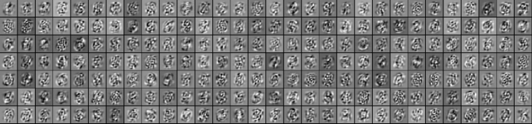
Figure 1: Some entries from the dictionary for RPCA with 1000 hidden units

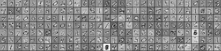
Figure 2: Some entries from the dictionary using the new k-sparse prior with 1000 hidden units and $k=20$

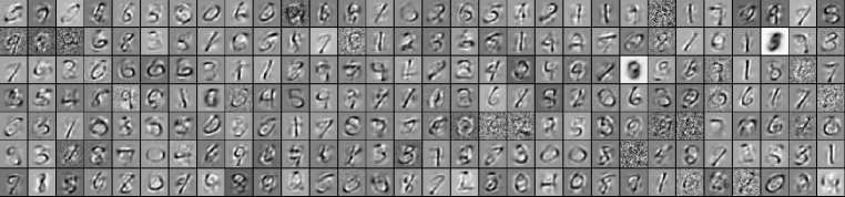
Figure 3: Some entries from the dictionary using the new k-sparse prior with 1000 hidden units and $k=40$

		k=100	k=40	k=20
RPCA	7.80
k-sparse		2.87	3.27	3.45

Table 1: Results for logistic regression on the sparse codes of the efficient RPCA and k-sparse implementation.

8 Conclusion and future work

The classification quality of an efficient version of RPCA has been presented. An additional addon was presented solving several problems that arised during the usage of RPCA. This solution consists of changing the regularizer from a l1-norm to a completely new prior using the k-sparse function. Due to the mathematical derivation of the network structure from the objective function this new prior automatically incoperates itself inside the transfer function. Now the sparse code has a much sparser structure but also the parameter decision got much more stable. This new k-sparse coding model resulted in much lower classification errors than the original efficient RPCA version.

Future work consists of testing this new k-sparse norm as prior also for regular sparse coding or non-negative matrix factorization. Another application could be to use it as regularizer for any other machine learning algorithm.