Influence of adaptive mesh refinement and the hydro solver on shear-induced mass stripping in a minor-merger scenario

Abstract

We compare two different codes for simulations of cosmological structure formation to investigate the sensitivity of hydrodynamical instabilities to numerics, in particular, the hydro solver and the application of adaptive mesh refinement (AMR). As a simple test problem, we consider an initially spherical gas cloud in a wind, which is an idealized model for the merger of a subcluster or galaxy with a big cluster. Based on an entropy criterion, we calculate the mass stripping from the subcluster as a function of time. Moreover, the turbulent velocity field is analyzed with a multi-scale filtering technique. We find remarkable differences between the commonly used PPM solver with directional splitting in the Enzo code and an unsplit variant of PPM in the Nyx code, which demonstrates that different codes can converge to systematically different solutions even when using uniform grids. For the test case of an unbound cloud, AMR simulations reproduce uniform-grid results for the mass stripping quite well, although the flow realizations can differ substantially. If the cloud is bound by a static gravitational potential, however, we find strong sensitivity to spurious fluctuations which are induced at the cutoff radius of the potential and amplified by the bow shock. This gives rise to substantial deviations between uniform-grid and AMR runs performed with Enzo, while the mass stripping in Nyx simulations of the subcluster is nearly independent of numerical resolution and AMR. Although many factors related to numerics are involved, our study indicates that unsplit solvers with advanced flux limiters help to reduce grid effects and to keep numerical noise under control, which is important for hydrodynamical instabilities and turbulent flows.

1 Introduction and astrophysical motivation

In the widely accepted paradigm of hierarchical formation of cosmic structure, large virialized objects like clusters of galaxies grow by accretion of smaller subclusters. In this process, which proceeds up to the current epoch, the merging of halos and subhalos is believed to be an important source of turbulence in the intra-cluster medium (hereafter ICM; e. g., Paul et al., 2011; Vazza et al., 2011) together with other mechanisms like the baroclinic injection of vorticity at curved shocks (Kang et al., 2007; Iapichino and Brüggen, 2012), outflows of active galactic nuclei (Heinz et al., 2006; Sijacki and Springel, 2006; Brüggen et al., 2009) and the motion of single galaxies through the ICM (Kim, 2007; Ruszkowski and Oh, 2011). The importance of cluster mergers goes beyond being mere stirring agents in the ICM. For example, they are strongly correlated with the occurrence of central cluster diffuse radio emission (radio halos; Cassano et al. 2010) via some still debated mechanism of cosmic ray acceleration (Brunetti and Jones, 2014). Moreover, major mergers launch shock waves in the ICM, which are observed as brightness and temperature edges in X-ray images (Markevitch, 2010). There is also the prospect of measuring turbulence with the up-coming Astro-H mission (Biffi et al., 2013; Shang and Oh, 2013).

The role of mergers as injectors of bulk flow and turbulence in the ICM has been recognized in hydrodynamical simulations of the build-up of galaxy clusters (e. g., Ricker, 1998; Norman and Bryan, 1999; Iapichino and Niemeyer, 2008; Vazza et al., 2011, 2012; Miniati, 2014). Complementary to cosmological simulations starting from realistic initial conditions, idealised cluster simulations are useful to study mergers in a simplified setup and with a better control on the problem parameters (Roettiger et al., 1996; Ricker and Sarazin, 2001; McCarthy et al., 2007). A special subclass of cluster mergers is constituted by minor mergers, where one the merging objects has a much smaller mass than the other. Although these processes do not have the same impact on the energy budget of the ICM as major mergers, they are interesting in their own right. For example, they are associated with observed structures like merger cold fronts (Markevitch and Vikhlinin, 2007; Russell et al., 2014). During minor mergers, the interface between the host ICM and the subcluster is subject to the Kelvin-Helmholtz instability, which results in gas stripping and injection of turbulence in the downstream region (Subramanian et al., 2006; Russell et al., 2014; Eckert et al., 2014). This process has been noticed in full cosmological simulations (Iapichino and Niemeyer, 2008; Maier et al., 2009) and has been studied in greater detail by means of idealised setups, following the infall of a low-mass subcluster or an elliptical galaxy into the static ICM of a big cluster as it is seen from an observer moving with the subcluster (Heinz et al., 2003; Takizawa, 2005; Xiang et al., 2007; Asai et al., 2007; Dursi and Pfrommer, 2008; Roediger et al., 2014a, b).

The study of Iapichino et al. (2008) belongs to the latter class of simulations. A particularly interesting aspect of this study is the transition from laminar flow to turbulence in the boundary layer of the subcluster, which is difficult to tackle for compressible hydro solvers with numerical viscosity. In this article, we further elaborate on this computational problem by comparing simulations carried out with the cosmological fluid dynamics codes Enzo and Nyx, which implement a split and an unsplit variant of the widely applied piecewise parabolic method (PPM, Colella and Woodward 1984). In order to gain a clearer insight into the simulations performed with the setup from Iapichino et al. (2008), we also address the simpler case of an unbound cloud in a wind as in Agertz et al. (2007). In this case, the cloud is initially defined as a spherical region of higher gas density in pressure equilibrium with the ambient medium. The code comparison by Agertz et al. (2007) was a seminal work that demonstrated striking differences between smoothed particle hydrodynamics (SPH) and grid-based codes.

Another question concerns an assumption that is often taken for granted in computational astrophysics, namely the equivalence between a run performed with a uniform grid and the corresponding simulation using adaptive mesh refinement (AMR) at the same effective spatial resolution. Recently, Miniati (2014) has questioned that dynamic refinement reproduces turbulent fluid properties, particularly if the refinement method is based on keeping the mass in a cell roughly constant. Thus, we want to investigate in a systematic way under which conditions statistical agreement between computations with AMR and uniform grids at the same effective resolutions can be achieved. By computing statistics related to the stripping of mass from the subcluster and by investigating the flow structure, a significant impact of refinement strategies in AMR simulations has been shown by Iapichino et al. (2008). In particular, AMR based on local gradients of density or temperature is not able to follow the formation of the turbulent subcluster wake, whereas this is possible with criteria based on the variability of structural invariants of the flow. This means that thresholds for refinement are calculated from statistical moments of scalars such as the squared vorticity (cf. Schmidt et al. 2009; Schmidt 2014).

To infer the impact of the different hydro solvers implemented in Enzo and in Nyx and to compare uniform-grid versus AMR runs, we compute the mass stripped from the subcluster as a function of time. For the definition of the cloud mass, we propose a criterion that is based on an entropy threshold. We find systematic differences, which are further analyzed by means of the multi-scale filtering approach of Vazza et al. (2012). After explaining our methodology in Section 2 in more detail, the results for the simple cloud without gravity and the subcluster are presented in Sections 3 and 4, respectively. Our conclusions are presented in the last section.

2 Numerical methods and simulations

We consider both gravitationally bound and unbound variants of the cloud in a wind, as defined by Iapichino et al. (2008). As initial condition, we set a spherically symmetric isothermal cloud in pressure equilibrium with a homogeneous background medium with temperature $k_{\rm B}T_{\rm b}=8.0\;\mathrm{keV}$ and density $\rho_{\rm b}=7.9\times 10^{-28}\;\mathrm{g\,cm^{-3}}$. In the simple case of an unbound cloud, we assume a sphere of radius $250\;\mathrm{kpc}$ with constant density $\rho_{\rm c}=6.3\times 10^{-27}\;\mathrm{g\,cm^{-3}}$. The condition of pressure equilibrium implies a temperature $k_{\rm B}T_{\rm c}=1.0\;\mathrm{keV}$ inside the cloud. To produce a wind in $x$-direction, an inflowing boundary condition with a uniform velocity $v_{\rm b}=1.6\times 10^{3}\,\mathrm{km\,s^{-1}}$ is imposed at the left face of the domain. The boundary conditions at the other faces of the domain are outflowing. Since the cloud is not anchored by a gravitational well, it drifts in the downstream direction. For this reason, we use an elongated box of size $16\times 4\times 4\;\mathrm{Mpc}$. Apart from the chosen scales, this setup is similar to the blob test of Agertz et al. (2007).

Iapichino et al. (2008), on the other hand, assume that the cloud is bound by an external gravitational potential, which corresponds to a static dark-matter halo with a King profile:

$$\rho_{\mathrm{dm}}(r)=\rho_{\mathrm{dm,c}}\left[1+\left(\frac{r}{r_{\rm core}}\right)^{2}\right]^{-3/2}\,.$$ (1)

The initial density profile of the cloud is obtained by integrating the equation of hydrostatic equilibrium for the central density $\rho_{\rm c}=0.1\rho_{\mathrm{dm,c}}=6.3\times 10^{-27}\,\mathrm{g\,cm^{-3}}$, constant temperature $k_{\rm B}T_{\rm b}=3.65\;\mathrm{keV}$, and the core radius $r_{\rm core}=250\,\mathrm{kpc}$. We use the same setup here, except for a cutoff at the radius $r_{\rm max}=6r_{\rm core}$. The Cartesian coordinates of the cloud centre ($r=0$) are $(0.4,0.5,0.5)\times 4\;\mathrm{Mpc}$ in a cubic domain of $4\;\mathrm{Mpc}$ linear size. For $r>r_{\rm max}$, the gravitational acceleration is set to zero and the state is given by the state of the background medium. The cutoff is necessary because of the applied boundary conditions, which are the same as in the case without gravity. In principle, the wind could be assumed to be in a turbulent state. However, the properties of turbulence in the ICM are quite uncertain and there is no suitable method that would allow us to self-consistently add turbulence to the background medium. Artificially added perturbations at the inflow boundary would largely decay before the could reach the cloud. Consequently, we consider only turbulence that is produced by hydrodynamical instabilities in this study. This has furthermore the advantage that perturbations of numerical origin can be investigated in a clear manner. For brevity, we subsequently refer to the cloud with static gravitational potential as “subcluster”.

To compute the gas-dynamical evolution for an adiabatic equation of state with $\gamma=5/3$, we apply the cosmological AMR codes Enzo (ascl:1010.072; O’Shea et al. 2005; Bryan et al. 2014) and Nyx (Almgren et al., 2013). As described in the method paper by Bryan et al. (2014), Enzo uses directionally split PPM (Colella and Woodward, 1984). A variety of Riemann solvers are available in the current code version. We are using the default two-shock approximation (see Toro, 1997), with the Harten-Lax-van Leer scheme as fallback. We do not make use of the dual energy formalism, as the flow in the problem under consideration does not have Mach numbers much higher than unity. The Nyx code, as described in Almgren et al. (2013), features an unsplit version of PPM with full corner coupling (Miller and Colella, 2002). The Riemann solver in Nyx also uses a two-shock approximation. Differences between Enzo and Nyx include the split vs unsplit nature of the integrator, as well as the details of the reference state used in the PPM profile, the flux limiters, and the exact discretization of the gravitational source terms in the energy equation. In addition, the construction of refined grid patches in both codes follows the same clustering algorithm as described in Berger and Rigoutsos (1992) but Nyx, unlike Enzo, does not require that each child grid have a unique parent. Moreover, there are different control parameters to constrain the size of grid patches as well as the buffer zones between consecutive refinement levels. Finally, the solution procedure for the multilevel gravitational field differs between the two codes. Both codes feature N-body solvers to compute the evolution of dark matter, but we use only a static gravitational potential. Self-gravity of the gas is not included either because the halo is the main source of gravity. Also other physical processes such as viscous damping, cooling, star formation, and magnetic fields are not considered here.

As shown by Iapichino et al. (2008), simple refinement by overdensity does not fully capture the frontal bow shock and the turbulent wake produced by vortex shedding from the cloud. For this reason, we apply refinement by the vorticity modulus and the rate of compression (Schmidt et al., 2009; Schmidt, 2014). The vorticity is the curl of the velocity, $\boldsymbol{\omega}=\boldsymbol{\nabla}\times\boldsymbol{v}$, and the rate of compression is the negative substantial time derivative of the divergence $d=\boldsymbol{\nabla}\cdot\boldsymbol{v}$. To compute the rate of compression, we evaluate the source terms in the dynamical equation for $d$, which follows by contracting the partial differential equation for the velocity with the divergence operator (see also Iapichino et al., 2011; Schmidt et al., 2013):

$$-\frac{\mathrm{D}d}{\mathrm{D}t}=\frac{1}{2}\left(|S|^{2}-\omega^{2}\right)+\boldsymbol{\nabla}\cdot\left(\frac{\boldsymbol{\nabla}P}{\rho}\right)-\boldsymbol{\nabla}\cdot\boldsymbol{g}_{\rm K}.$$ (2)

The first term on the right-hand side describes the competing effects of strain and vorticity, the following term accounts for the effect of the thermal gas pressure, and the last term corresponds to the gravity resulting from the King profile (see equation 1). For $q_{1}=\omega^{2}$ and $q_{2}=-\mathrm{D}d/\mathrm{D}t$, cells are tagged for refinement to the next higher level if

$$|q_{i}|\geq|\langle q_{i}\rangle_{n}|+\max\left(|\langle q_{i}\rangle_{n}|,\mathrm{std}_{n}q_{i}\right),$$ (3)

where the brackets $\langle\cdot\rangle_{n}$ denote the average over all cells at level $n$ and $\mathrm{std}_{n}q_{i}=\langle q_{i}^{2}\rangle_{n}-\langle q_{i}\rangle_{n}^{2}$ is the standard deviation from the average. The basic rationale of this method is that refinement should be triggered if the local value exceeds the typical fluctuation given by the standard deviation, but only if the fluctuation is significant, i. e., comparable to the mean or larger. Thus, we define the thresholds for refinement by level-wise statistics of the control variables vorticity and rate of compression, without any tunable parameters.

$N_{0}$	$n_{\rm max}$	AMR	$\Delta_{\rm min}\;[\mathrm{kpc}]$
unbound cloud
$512\times 128^{2}$	$0$	no	$31.3$
$512\times 128^{2}$	$1$	yes	$15.6$
$1024\times 256^{2}$	$0$	no	$15.6$
$512\times 128^{2}$	$2$	yes	$7.8$
$2048\times 512^{2}$	$0$	no	$7.8$
subcluster
$128^{3}$	$1$	yes	$15.6$
$256^{3}$	$0$	no	$15.6$
$128^{3}$	$2$	yes	$7.8$
$512^{3}$	$0$	no	$7.8$
$128^{3}$	$3$	yes	$3.9$

Table 1: Overview of simulation runs, ordered by increasing numerical resolution, where $N_{0}$ is the number of root-grid cells, $n_{\rm max}$ the maximum refinement level, and $\Delta_{\rm min}$ the cell size at highest refinement level.

We performed the simulations listed in Table 1, using both Enzo and Nyx. The smallest resolved length scale in the uniform-grid simulations with $2048\times 512^{2}$ (unbound cloud) or $512^{3}$ (subcluster) grid cells is $\Delta_{\rm min}\approx 7.8\;\mathrm{kpc}$. These simulations can be compared to AMR simulations with the same effective resolution, which is reached with root-grid resolutions of $512\times 128^{2}$ (unbound cloud) or $128^{3}$ (subcluster) at the second level of refinement. Since the domain volume for a given resolution is four times larger for the unbound cloud than for the subcluster, three levels of refinement ($\Delta_{\rm min}\approx 3.9\;\mathrm{kpc}$) were applied only in the case of the subcluster.

In order to better highlight the small-scale motions in the downstream of the stripped cloud, we employ a multi-scale filtering technique which makes no assumptions on the injection scale of chaotic motions (Vazza et al., 2012). The filter reconstructs the local mean velocity field around each cell by iteratively computing the local mean velocity field as

$$\overline{\boldsymbol{v}(L_{n})}=\frac{\sum_{i}(r<L_{n})w_{\rm i}\boldsymbol{v}_{i}}{\sum_{i}w_{i}},$$ (4)

where $w_{\rm i}$ is a weighting function (e. g., gas density or gas mass, but for our simulations we simply set $w_{\rm i}=1$ because of the small density contrast). The local small-scale velocity field is computed as $\delta\boldsymbol{v}(L_{\rm n})=\boldsymbol{v}-\overline{\boldsymbol{v}(L_{n})}$ for increasing values of $L_{n}$. The iterations are continued until the relative variation of the local turbulent velocity between two iterations is below the given tolerance parameter, which based on our tests we set to $\epsilon=0.1$. Additionally, the scheme stops iterating whenever the skewness of the velocity distribution with a stencil of $8^{3}$ cells is found to be larger than a tolerance parameter, as specified in Vazza et al. (2012). As final output, the maximum scale $L$ of turbulent eddies around each cell and the local turbulent velocity $\delta\boldsymbol{v}(L)$ are obtained.

3 Unbound cloud

The evolution of the unbound cloud in the AMR run with the highest resolution is illustrated in Figure 1. As reported by Agertz et al. (2007), the initially spherical cloud is rapidly compressed into an oblate shape. Because of the supersonic wind, a bow shock forms in front of the cloud. Subsequently, a complex pattern of shocks and interfering pressure waves emerges, for which the rate of compression is an excellent indicator. After a few Gyr, the waves are mostly dissipated. One can also see the formation of vortices and the stripping of gas from the cloud. This is a consequence of Kelvin-Helmholtz instabilities in the shear layers between the background flow and the cloud interior and Rayleigh-Taylor instabilities due to the acceleration of the denser cloud material by the low-density wind (see Agertz et al. 2007 for a detailed discussion of these processes). As a result, a turbulent mushroom-like structures develops, which is dragged by the wind in downstream direction. The density contrast gradually decreases because of the mixing of the cloud material into the background medium.

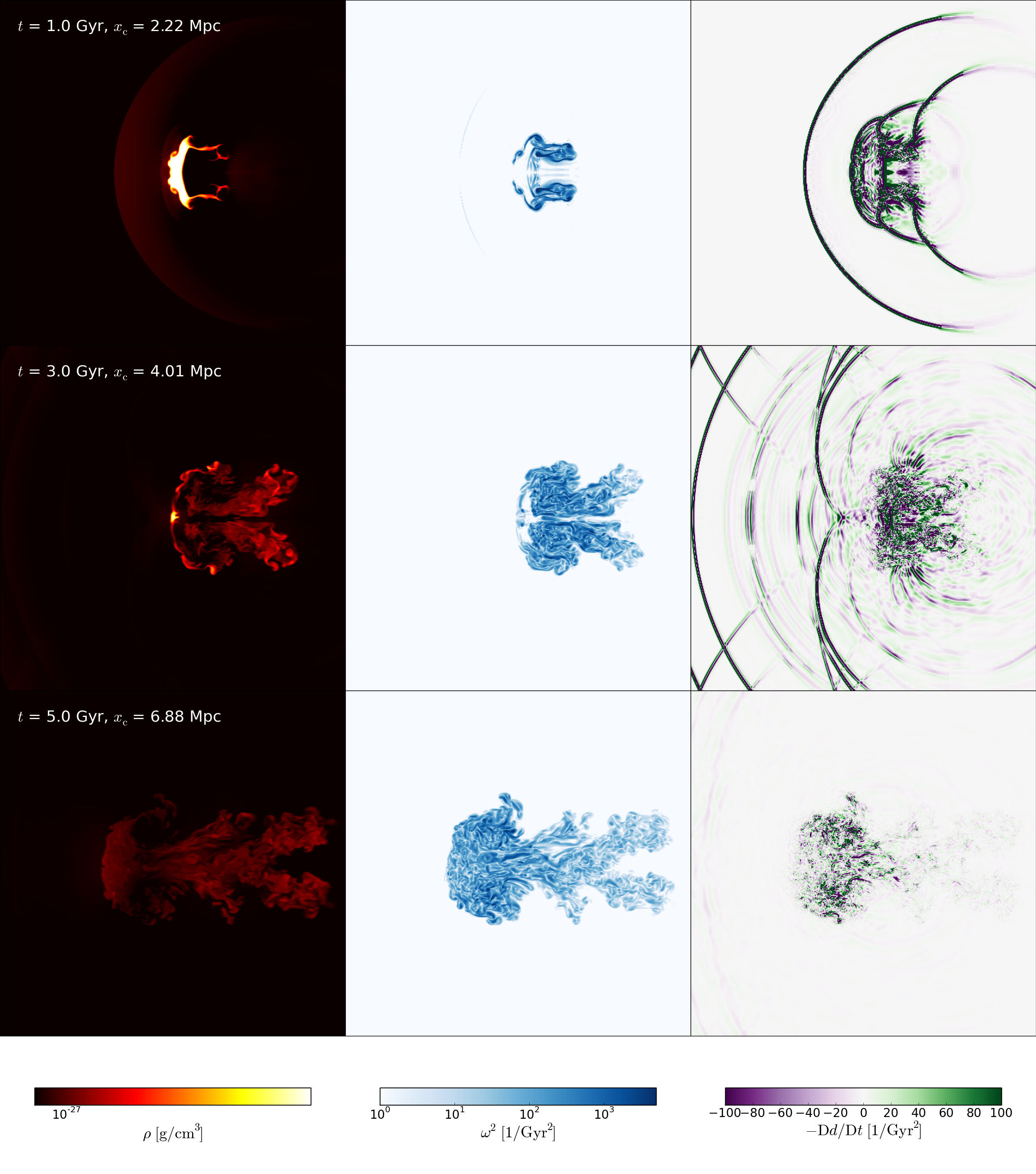
Figure 1: Highest-resolution AMR simulation of the unbound cloud performed with the code Nyx. Shown are the mass density $\rho$ (logarithmic scale), the squared vorticity modulus $\omega^{2}$, and the rate of compression $-\mathrm{D}d/\mathrm{d}t$ (see equation 2) in a $4\;\mathrm{Mpc}\times 4\;\mathrm{Mpc}$ region of the $xy$-plane for $t=1.0\;\mathrm{Gyr}$ (top), $3.0\;\mathrm{Gyr}$ (middle), and $5.0\;\mathrm{Gyr}$ (bottom). To follow the downstream drift of the cloud, the displayed region is centered at the coordinate $x_{\rm c}$ in $x$-direction.

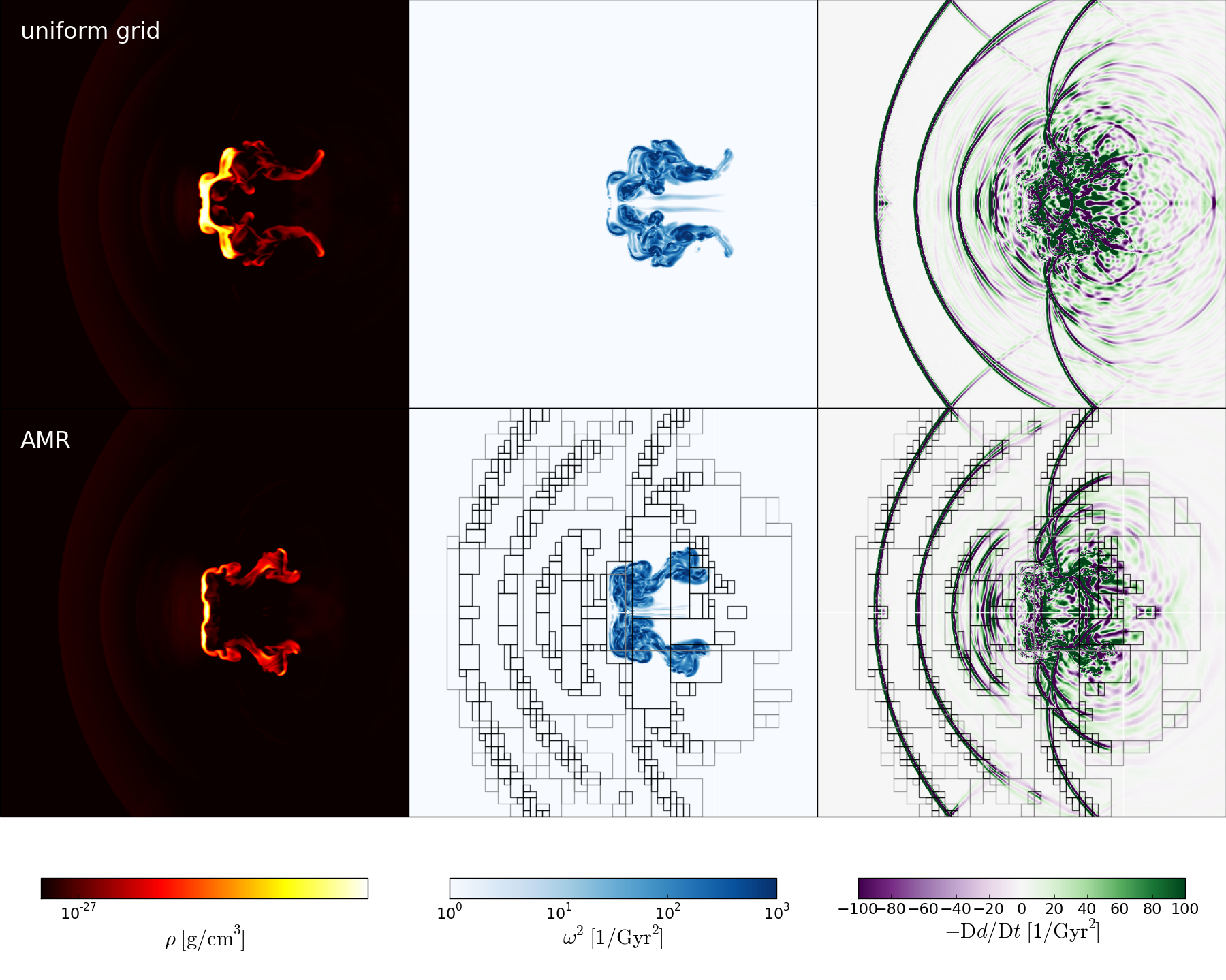
Figure 2: Highest-resolution uniform-grid (top) and AMR (bottom) simulations of the unbound cloud performed with the code Nyx. Shown are slices of the mass density $\rho$, the squared vorticity modulus $\omega^{2}$, and the rate of compression $-\mathrm{D}d/\mathrm{d}t$ for $t=2.0\;\mathrm{Gyr}$ (i. e., a stage in between the top and middle rows in Figure 1). The boxes in the bottom panels indicate grid patches produced by AMR at level 1 (gray boxes) and level 2 (black boxes). For example, from left to right the resolution increases upstream of the the first bow shock from level 0 to level 2 around the shock, then decreases to level 1 and increases again to level 2 around the second shock, etc.

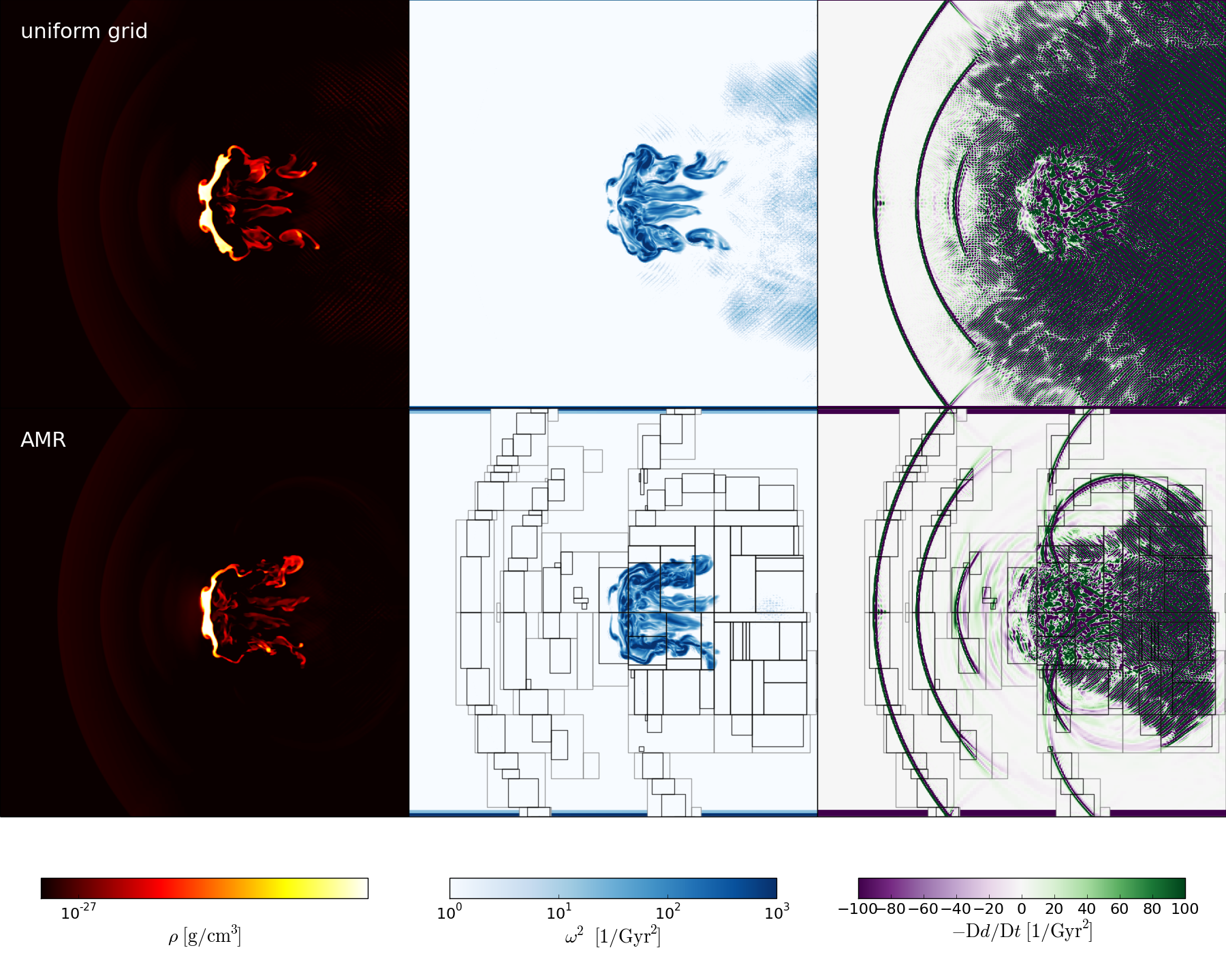
Figure 3: The same as in Figure 2 for the corresponding simulations performed with Enzo.

If a uniform grid with the same effective resolution as in the AMR run is used, the flow evolution is qualitatively similar. However, the comparison between the uniform-grid and AMR runs at $t=2.0\;\mathrm{Gyr}$ in Figure 2 shows palpable differences in the cloud morphology (density slices) and the flow structure (vorticity slices). In particular, it appears that more gas is ablated from the frontal cap in the AMR run. Shocks, which appear as large arcs in the slices of the compression rate, are nearly identical in both runs. Slices from the corresponding Enzo runs at the same instant of time are plotted in Figure 3. Compared to the Nyx runs, the shape of the cloud is markedly different. However, the deviation of the AMR run from the uniform-grid run appears to be less pronounced for Enzo. Deviations are, of course, inevitable because of the non-linear evolution of the flow instabilities, but the differences between the various runs are stronger than what one might expect. In the fully turbulent regime, after the cloud has largely dissolved, the differences in the flow structure tend to be alleviated (see Figure 4 for $t=4.0\;\mathrm{Gyr}$). This is possibly a consequence of the randomization caused by turbulence.

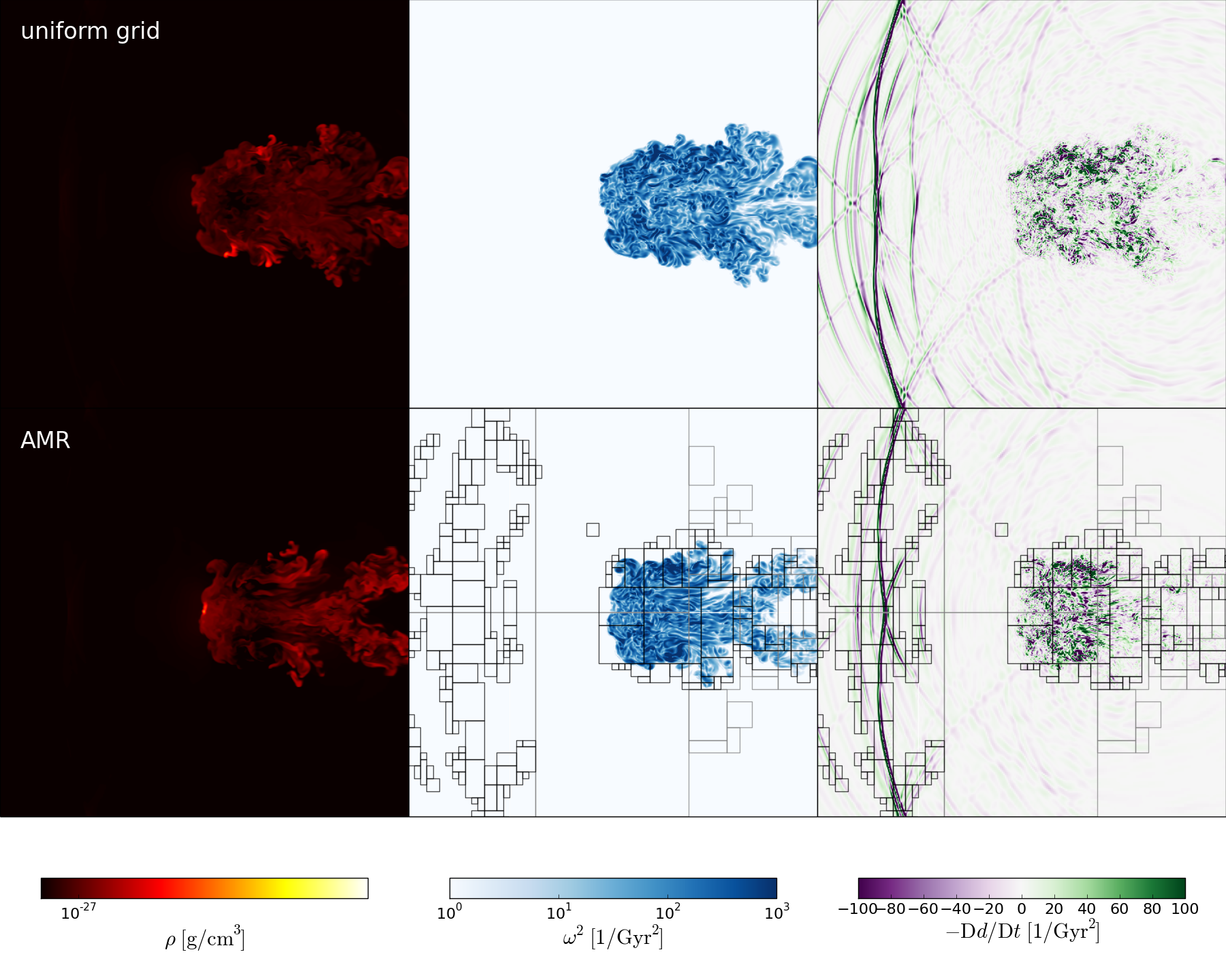
Figure 4: The same as in Figure 2 for the Nyx simulation at

$t=4.0\;\mathrm{Gyr}$.

A major discrepancy between Nyx and Enzo that becomes apparent in the slices shown in Figures 2 and 3 is the interference pattern of waves in the surroundings of the cloud. In both cases, the compression rate indicates pressure waves produced by the collision of the incoming gas with the denser cloud. However, while the wavelength separating local maxima or minima of $-\mathrm{D}d/\mathrm{d}t$ is clearly larger for Nyx, the wave amplitude is much smaller: $|\mathrm{D}d/\mathrm{d}t|\sim 10$ for Nyx, but $|\mathrm{D}d/\mathrm{d}t|\gg 100$ for Enzo. Apart from that, the wavelength apparently changes with the grid resolution in the case of Enzo (not shown here). This suggests that the waves in the Enzo runs might at least partially be of numerical origin.

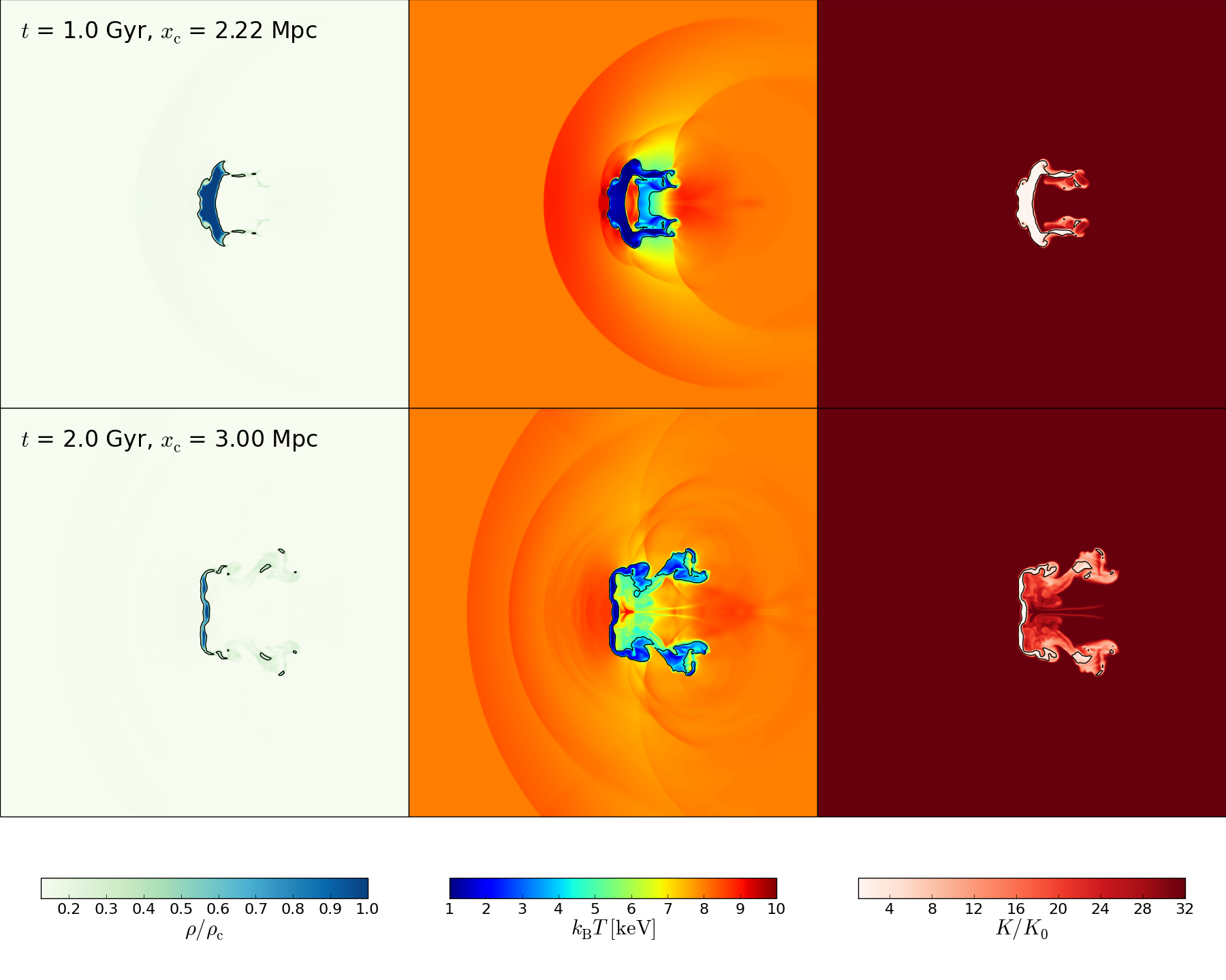
Figure 5: Slices of the density, temperature, and entropy for the highest-resolution AMR simulation performed with Nyx at two different instants. The density and entropy are normalized to the initial central density $\rho_{\rm c}$ and entropy $K_{0}$, respectively, of the cloud. Isosurfaces for $\rho/\rho_{\rm c}=0.32$ (left), $T=4.5\;\mathrm{keV}$ (middle), and $K/K_{0}=8.0$ (right) are indicated by black contour lines. The slices are centered at coordinates $x_{\rm c}$ in $x$-direction, as in Figures 1 and 4.

3.1 Mass stripping

An important question is whether robust statistics, which are not too sensitive to the numerical realization, can be inferred from the simulations. To characterize the mass stripping from the cloud, Agertz et al. (2007) and Iapichino et al. (2008) use the total mass of gas that has temperatures below and densities above given thresholds as statistical measure. The density and temperature thresholds chosen by Agertz et al. (2007) are $0.64\rho_{\rm c}$ and $0.9T_{\rm b}$, while Iapichino et al. (2008) set a lower threshold of $0.32\rho_{\rm c}$ for the density. The regions with $\rho/\rho_{\rm c}\geq 0.32$ at $t=1.0$ and $2.0\;\mathrm{Gyr}$ are shown for the Nyx AMR simulation with two levels of refinement in Figure 5. The temperature slices in the middle make clear that the threshold $0.9k_{\rm B}T_{\rm b}=7.2\;\mathrm{keV}$ encloses a lot of low-density material from the ambient medium, which is heated by adiabatic compression. For this reason, we consider a lower maximal temperature of $T_{\rm c}+0.5(T_{\rm b}-T_{\rm c})\approx 0.56T_{\rm b}$, corresponding to $4.5\;\mathrm{keV}$, to constrain the cloud interior. The resulting time evolution of the total mass $M(t)$ of the gas with $\rho/\rho_{\rm c}\geq 0.32$ and $k_{\rm B}T\leq 4.5\;\mathrm{keV}$ is plotted as dot-dashed line in Figure 6. At $t=1\;\mathrm{Gyr}$, the cloud is compressed and deformed (see Figure 5), but still retains a large fraction of the initial mass. During a phase of rapid mass loss, the cloud is fragmented and about half of its initial mass is mixed into the background medium. Eventually, after about $3\;\mathrm{Gyr}$, the cloud has lost most of its mass. Compared to the thresholds $0.64\rho_{\rm c}$ and $7.2\;\mathrm{keV}$ as in Agertz et al. (2007), $M(t)$ initially decreases more gradually and the lifetime of the cloud is longer.

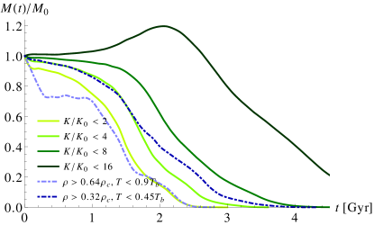
Figure 6: Time evolution of the cloud mass for different choices of the entropy threshold (solid lines) for the Nyx AMR simulation with one level of refinement. The dot-dashed lines are obtained if the cloud is defined by a lower threshold for the density and an upper threshold for the temperature.

In contrast to the temperature, the entropy is not increased by adiabatic compression (with the exception of shocks). However, the entropy of the gas in the cloud is raised as it is mixed into the background medium by turbulence. This suggests that the cloud interior can be defined by an entropy threshold. Indeed, the low-entropy material of the cloud stands out against the background medium in the slices of the entropy shown in Figure 5. Thus, we define the cloud interior by the criterion

$$K=\frac{T}{\rho^{2/3}}\leq K_{\rm max}=fK_{0},$$ (5)

where $K_{0}=T_{\rm c}/\rho_{\rm c}^{2/3}$ is the initial entropy in the centre of the cloud and $f>1$ a dimensionless factor. The cloud masses defined by the above criterion with $f=2$, $4$, $8$, and $16$ are plotted as functions of time in Figure 6. The cloud mass defined by $\rho/\rho_{\rm c}\geq 0.32$ and $k_{\rm B}T\leq 4.5\;\mathrm{keV}$ falls in between the cases $f=4$ and $f=8$. For $f=2$, there is a sudden drop of the cloud mass just after $t=0$, while $f=16$ does not sufficiently constrain the cloud interior to obtain a monotonously decreasing mass. We choose $f=8$ as fiducial value for our analysis because the mass is smoothly ramped down over a relatively long period of $4\;\mathrm{Gyr}$ (the corresponding entropy contours are overplotted in Figure 5).

The mass statistics for the simulations listed in the upper part of Table 1 are plotted in Figure 7. One can see in the left plot that the mass stripping in the Nyx simulations is relatively robust for different resolutions as well as uniform-grid vs. AMR simulations, although there is a relatively large deviation of the run with a uniform grid at maximal resolution ($\Delta_{\rm min}=7.8\;\mathrm{kpc}$), particularly in the early mass-loss phase between $1$ and $2\;\mathrm{Gyr}$. This might be a consequence of the differences in the cloud morphology that can be seen in Figure 2. The less pronounced differences in the corresponding Enzo simulations (see Figure 3) are reflected by a better agreement of $M(t)$ between the runs with the same effective resolution (right plot in Figure 7). However, not only is the dependence on effective resolution stronger in the case of Enzo, but there are striking systematic differences: The mass stripping progresses clearly faster if Nyx is used. This behavior is further investigated for the subcluster in Section 4.

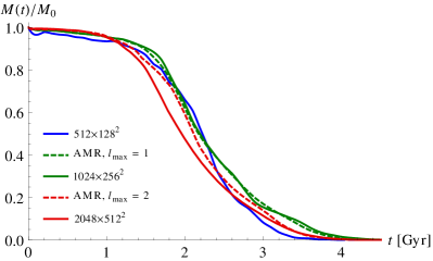
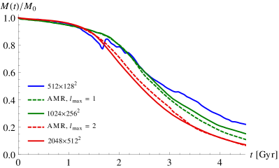
Figure 7: Time evolution of the cloud mass in AMR simulations (dashed lines) with $n_{\rm max}$ levels of refinement and in uniform-grid simulations (solid lines) with different resolutions for Nyx (left) and Enzo (right). Simulations with the same effective resolutions are shown in the same colours (online version). For all curves, the cloud interior is defined by $K/K_{0}<8$.

Figure 8: Maps of total velocity modulus (in units of cm/s) for a slice crossing the middle plane of the unbound cloud runs at time $t=3\;\mathrm{Gyr}$. The top panels show the maps for Enzo with a uniform grid of $1024\times 256^{2}$ cells (left) and with AMR, using 1 level of refinement (right). The bottom panels show the corresponding results for Nyx. The additional dashed selections display the subregions used for our analysis of turbulent velocity statistics.

Figure 9: Maps of turbulent velocity modulus relative to the upstream wind velocity $v_{\rm b}$ for the same runs and selections as in Fig. 8.

3.2 Turbulent velocity

To obtain a better understanding of the differences between the codes, we analyze turbulent flow statistics. Figure 8 shows the total velocity map for a slice through the middle plane of the unbound cloud runs (we consider here the intermediate resolution of $1024\times 256^{2}$ and the corresponding AMR run with 1 level of refinement) at the epoch of $3\;\mathrm{Gyr}$. Apart from the shock waves in the upstream region, the velocity field in the uniform-grid Enzo run shows a prominent pattern of small-scale perturbations, which fills a much larger volume than in the corresponding AMR case. This pattern also can be seen in the compression rate (not plotted here). The fluctuations are better highlighted by the filtering of velocity data with the algorithm presented in Section 2. For the same instant of time, Figure 9 presents slices showing the modulus of the turbulent field $\delta\boldsymbol{v}(L)$ resulting from the filtering algorithm. As expected, the filtering procedure reveals a ”noisy” pattern of interfering small-scale waves in Enzo, just downstream of the blob in the AMR run and even at the sides of the blob in the run with a uniform grid. These small-scale waves are totally absent in Nyx runs, where only a coherent pattern of sound waves originating from the cloud can be seen. Another interesting difference between the two codes is that the turbulent velocity field in the cloud interior and wake appears to be more irregular in the Nyx run. The higher symmetry for Enzo is possibly a consequence of the propensity of Kelvin-Helmholtz rolls to get aligned with the grid if directional splitting is used. Since the unsplit solver implemented in Nyx reduces the influence of the grid directions, it is conceivable that the turbulent flow randomizes faster. This could also explain the faster mass stripping in the Nyx runs (see Section 3.1).

The turbulent velocity profiles plotted in Fig. 10 are obtained by calculating the root mean square (rms) velocity for slices perpendicular to the wind direction. While the profiles agree within a few percent for most of the volume, the Enzo data show a striking excess of velocity dispersion downstream of the cloud. The corresponding region is marked as region B in Fig. 8. Figure 11 shows the volume distribution of correlation scales $L$ in the flow, as given by the filtering algorithm of Section 2. In comparison to Nyx, the Enzo run appears to have an excess of small-scale structure, which can be associated with the ”noisy” pattern in Fig. 9. For scales larger than about 25 cells, the two codes produce very similar distributions, confirming that the largest scales in the flow are reconstructed in a very similar way.

We further investigated the properties of the velocity field by computing 3D power spectra and second-order structure functions of the total (unfiltered) velocity field, defined as $S_{2}(l)=\langle|\delta\boldsymbol{v}(l)|^{2}\rangle$, where $\delta\boldsymbol{v}(l)$ is the velocity difference between two points separated by a distance $l$. For the spectra and structure functions, we selected two cubic subregions with $256^{3}$ cells in the simulation domain, as shown in Fig. 8. Region A contains the cloud and most of the turbulent wake, whereas the noisy pattern detected in the Enzo runs is encompassed by region B. The structure functions were computed for $10^{8}$ randomly chosen pairs of cells within each region, while the power spectra were computed with a standard FFT approach, assuming periodic boundary conditions. The results are shown in Fig. 12. For region A, the power spectra and structure functions obtained with the different codes are in good agreement for low to intermediate wavenumbers and length scales larger than a few $\Delta_{\rm min}$, respectively, regardless of using AMR or a uniform grid. However, there is a pronounced spike around $k\sim 70$, where $k=1$ corresponds to the size of the whole region. This indicates the onset of small-scale velocity fluctuations around the cloud in the uniform-grid Enzo run (see left top plot in Fig. 8). The slope of the spectra is roughly consistent with a Kolmogorov spectrum for intermediate wave numbers. However, the structure functions show no indication of a power law at all. Since the flow in subregion A is a mixture of turbulence and the surrounding wind, a clean power law cannot be expected. Apart from that, the numerical resolution is too low to resolve inertial-range scaling in the turbulent wake.

Even more striking differences between Enzo and Nyx are measured in region B (bottom plots in Fig. 12), where the noisy pattern of small-scale waves observed in Fig. 8 produces a very prominent peak for wavenumbers $k\sim 30$ to $100$ (i. e., scales of $2$ to $5$ grid cells). Since there are only pressure waves, but hardly any turbulence in this region, the spectrum should fall off steeply with the wave number, which is indeed seen for Nyx. The differences between the second-order structure functions in region B (lower right plot in Fig. 12) are even more pronounced. Compared to Nyx, the structure functions calculated from the Enzo data are almost flat and much larger in magnitude. However, the peak-like features that can be seen in the power spectra are not present. Possibly, the rapid fluctuations associated with the small-scale waves tend to be correlated over a few cells such that their contribution to $\delta\boldsymbol{v}(l)$ is suppressed. Moreover, the structure functions are very coarse for low $l$ compared to the large number of narrow wavenumber bins for high $k$. This might also obscure the peaks. There is no doubt, however, that the two codes produce substantially different levels of non-turbulent, noisy fluctuations, particularly in region B.

Figure 10: Profiles of the root mean square velocities within slices perpendicular to the wind direction for the same datasets as in Figure 9 ($t=3\;\mathrm{Gyr}$). The velocities are normalised to the upstream wind velocity, $v_{\rm b}$, in both cases.

Figure 11: Volume fractions of correlation scales in the flow (as reconstructed by the filtering algorithm explained in Section 2) for the datasets shown in Figure 9 ($t=3\;\mathrm{Gyr}$).

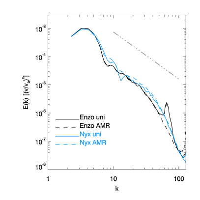
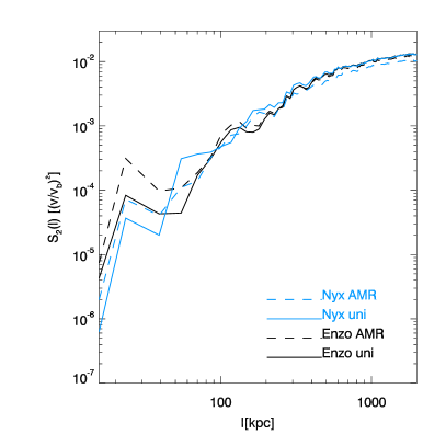
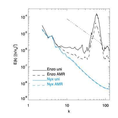
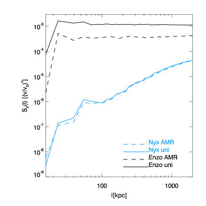
Figure 12: Power spectra of the velocity field (left panels) and second order structure functions (right panels) for two subvolumes of the computational domain at time $t=3.0\;\mathrm{Gyr}$ for the various Enzo and Nyx runs with a resolution of $15.6\;\mathrm{kpc}$ (see Table 1). Region A (top panels) is cloud-centered, while region B (bottom panels) contains the noisy pattern observed downstream in the Enzo run. The dot-dashed grey line shows the Kolmogorov slope ($k^{-5/3}$).

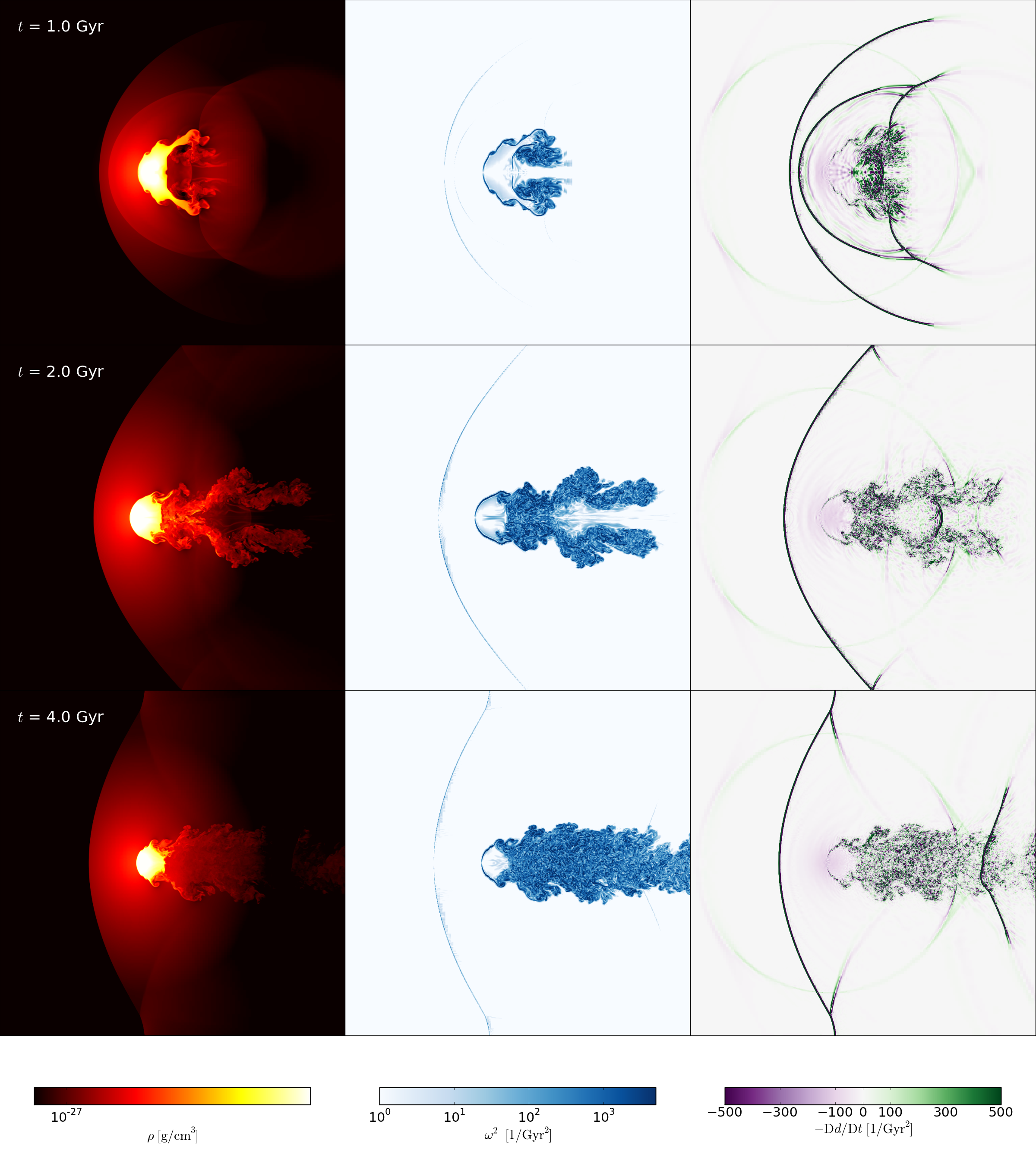
Figure 13: Highest-resolution AMR simulation of the subcluster performed with the code Nyx. Shown are slices of the mass density $\rho$, the squared vorticity modulus $\omega^{2}$, and the rate of compression $-\mathrm{D}d/\mathrm{d}t$ for $t=1.0\,\mathrm{Gyr}$ (top), $2.0\,\mathrm{Gyr}$ (middle), and $4.0\,\mathrm{Gyr}$ (bottom).

4 Subcluster

The evolution of the subcluster, i. e., the bound cloud in a static gravitational potential, is illustrated in Fig. 13 for the Nyx AMR simulation with three levels of refinement. As in the case of the unbound cloud, one can see that the initially spherical subcluster is deformed by the ram-pressure of the wind after $1\;\mathrm{Gyr}$ (top panels) and mass is stripped from the cloud by vortex shedding. However, the subsequent evolution is very different, as the subcluster is anchored by gravity. The gravitational potential produces a negative contribution to the rate of compression (see equation 2), which is visible near the center in the right panels. Also the cutoff of the potential at radius $r_{\rm max}$ can be discerned as a faint circle. Much stronger compression is caused by shocks and compressible turbulent fluctuations. At $t=2\;\mathrm{Gyr}$ (middle panels), there is a nearly stationary bow shock in front of the cloud and a turbulent wake begins to form. The final state at $t=4\;\mathrm{Gyr}$, when the simulation is terminated, is shown in the bottom panels. At this stage, the flow in downstream direction behind the cloud is fully turbulent.

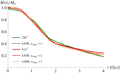
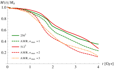
Figure 14: Mass of the gravitationally bound cloud as function of time in AMR (dashed and dot-dashed lines) and uniform-grid (solid lines) simulations with the resolutions listed in Table 1 for Nyx (left) and Enzo (right). Simulations with the same effective resolutions are shown in the same colour.

In Fig. 14, we compare the mass stripping in the different simulations performed with Nyx and Enzo (see Table 1). To define the cloud interior, we set $f=2$ in equation (5) because the entropy contrast between the cloud center and the background is smaller by about a factor of $4$ compared to the case without gravitational potential. Again we observe systematic differences between the two codes. Generally, the mass stripping progresses faster in the Nyx runs, with a steep decline from $t\approx 0.5\,\mathrm{Gyr}$ onwards. In this regime, instabilities at the cloud-background interface enter the non-linear regime and vortex shedding causes the ablation of relatively large chunks from the cloud (see top panels in Fig. 13). The mass-stripping levels off after about $2\,\mathrm{Gyr}$. The frontal surface of the cloud has become more or less smooth at this point and only small vortices are produced in a belt around the cloud (see middle panels in Fig. 13). For Enzo, we find a qualitatively similar behavior (right plot in Fig. 14), but the transition between the initial stripping and the turbulent wake regime is much more gradual. Similar to the simulations of the unbound cloud, the mass stripping progresses significantly slower compared to Nyx, particularly in the uniform-grid runs. This points to a genuine influence of the hydro solver. Moreover, the Enzo AMR runs show strong deviations from the corresponding uniform-grid runs with the same effective resolution. For Nyx, on the other hand, the mass stripping is nearly independent of numerical resolution and adaptivity. We further elaborate on these differences below.

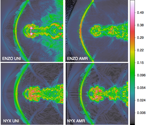
Figure 15: Maps of turbulent velocity modulus normalized by the upstream wind velocity $v_{\rm b}$ at $t=3\;\mathrm{Gyr}$ for simulations of the subcluster on a $512^{3}$ grid (left) and a $128^{3}$ root grid with 2 refinement levels (right).

As in the previous Section, we complement the mass statistics with an analysis of the turbulent velocity field by applying the multi-scale filtering method. A comparison of the turbulent velocities at $t=3\;\mathrm{Gyr}$ for an evolutionary stage in the the slow mass stripping phase highlights the differences between Nyx and Enzo, which are even more pronounced than in the case of the unbound cloud. For the $512^{3}$ uniform grid (left panels in Fig. 15), the flow has a rather high degree of symmetry in the Enzo run, while the subcluster appears to be more turbulent in the Nyx run. Moreover, Enzo produces a noisy pattern similar to what can be seen in Fig. 9 for the unbound cloud. One can also see that fluctuations are seeded when the wind enters the gravitational well. This spurious effect cannot be avoided because the circular boundary at radius $r_{\rm max}$ (see Section 2) cannot be mapped exactly to a Cartesian grid. As expected, directional splitting produces stronger fluctuations, particularly if AMR is used (top panels in Fig. 15). A conspicuous feature in the AMR run performed with Enzo is the strong fluctuations at the shock. It is likely that the noise induced by the gravitational cutoff upstream of the shock is amplified when it passes through the shock. This effect might contribute to the significantly stronger mass stripping from the cloud. For Nyx, on the other hand, the flow structure is similar in both runs (bottom panels in Fig. 15).

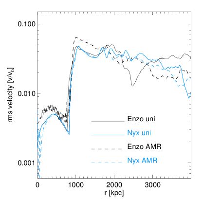
Figure 16: Profiles of the root mean square velocities within slices perpendicular to the wind direction for the same datasets as in Figure 17. The velocities are normalized to the upstream wind velocity $v_{\rm b}$.

Figure 16 shows the corresponding profiles of the rms velocity within planes perpendicular to the propagation axis of the wind. The profiles are quite similar in the upstream region, yet we see a small excess of pre-shock velocity fluctuations and a larger velocity dispersion at the shock edge around $x=1000\;\mathrm{kpc}$) in the Enzo AMR run. Moreover, the rms velocity is significantly larger between the bow shock and the cloud in this case, which is in agreement with the turbulent velocity maps shown in Fig. 15. Downstream of the subcluster core (initially centered at $x=1600\;\mathrm{kpc}$), the profiles are roughly comparable. However, the different flow structures in the Enzo and Nyx uniform-grid runs are reflected by differences in the turbulent velocity profiles.

Figure 17: Second-order structure function for the Enzo and Nyx for the same runs as in Figs. 15 and 16. The velocities are normalized by the upstream wind velocity $v_{\rm b}$.

The second-order structure functions plotted in Fig. 17 are peaked at length scales much greater than the core radius $r_{\rm core}=250\,\mathrm{kpc}$ of the subcluster. This indicates coherent structures that extend over the length of the tail of the subcluster, which is about $2000\;\mathrm{kpc}$. These structures contribute more to $S_{2}(l)$ in the case of the $512^{3}$ Enzo run than in the other runs. The structure functions are less stiff for both Enzo runs, which indicates an excess of small-scale structure, as suggested by the turbulent velocity maps in Fig. 15. To a lesser degree, differences can also be seen when comparing the two Nyx runs: AMR produces larger velocity fluctuations on small-scales, which is probably caused by spurious fluctuations due to grid refinement. Interestingly, the fluctuations on length scales larger than the core radius are slightly reduced. This suggests an enhanced decorrelation in the AMR run. In the case of Enzo, these differences are much more pronounced, which might explain the significantly stronger mass stripping and, as a consequence, the faster decrease of the size of the subcluster core compared to the constant-resolution case.

5 Conclusions

We performed numerical simulations of a simple cloud-in-a-wind problem with the cosmological AMR codes Enzo and Nyx. The setup follows Iapichino et al. (2008), who considered an idealized model for the minor merger of subcluster into the ICM of a big cluster. In this case, a static gravitational potential is applied to mimic the dark matter halo of the subcluster. As a variant of this problem, we also computed the evolution of an isothermal cloud without gravitational potential in an elongated box, similar to the scenario investigated by Agertz et al. (2007).

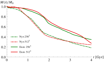
Figure 18: Comparisons of the mass stripping from the unbound cloud (left) and the subcluster (right) for the uniform-grid simulations with Enzo (solid lines) and Nyx (dot-dashed lines). Equivalent resolutions are shown in the same colors.

As in Iapichino et al. (2008) and Agertz et al. (2007), we computed the mass stripping from the cloud as basic statistical diagnostics of the effect of the wind on the cloud. An important difference to the previous studies is that we define the cloud interior by an entropy threshold rather than a lower bound on the density and an upper bound on the temperature. This leads to a smoother and almost monotonic evolution of the cloud mass. As shown in the plots in Fig. 18, the mass stripping reveals systematic differences between the codes for both the unbound and bound clouds even if numerical grids with uniform resolution are used. The sensitivity to resolution is generally stronger in the case of the unbound cloud (left plot), which is probably a consequence of the rapid destruction of the compact cloud by shear. Although the deviation between the two codes tends to become less for increasing resolution, the deviations are more pronounced than the differences between runs with given resolution. This trend can be seen very clearly for the subcluster (right plot), where the sensitivity to resolution is quite low for uniform-grid runs, but the evolution of the cloud mass differs substantially for Enzo and Nyx. The impact of the employed hydro solvers on the flow evolution is confirmed by analyzing statistical properties of the turbulent flow by means of the multi-scale filtering technique of Vazza et al. (2012). While the power spectra of turbulence on intermediate scales and the profiles of the RMS velocity fluctuation are generally in good agreement, we find deviations on scales of the order of the grid scale, which appear to be related to pronounced fluctuations in downstream regions in the case of Enzo.

The various discrepancies between the two codes we found in our study might stem from the following factors:

• Adaptive mesh refinement: Fine-coarse boundaries inevitably introduce some numerical noise. While the flow realizations clearly diverge when AMR simulations are compared to uniform-grid simulations, which is simply a consequence of non-linear dynamics, statistical properties are quite robust, at least for Nyx. In the case of the subcluster, we find large deviations between the AMR and uniform-grid runs performed with Enzo. Since this is not observed for the gravitationally unbound cloud, deviations might be caused by other sources of numerical noise, for example, the artificial cutoff of the gravitational potential, which is specific to the subcluster setup. The multi-scale filtering analysis suggests that fluctuations induced at cutoff radius are amplified by refinement in the vicinity of the bow shock, which in turn causes stronger mass stripping. In the Nyx AMR simulations, this effect appears to be much weaker.

• Directional splitting: Contrary to what one might expect, the unsplit solver implemented in Nyx tends to produce more asymmetric structures and faster mass stripping compared to the solver with directional splitting in Enzo. This can be understood as a consequence of the stronger alignment effects with the grid if directional splitting is used. Apart from that, also different flux limiters can play an important role for the evolution of instabilities, as demonstrated by Almgren et al. (2010) for the Rayleigh-Taylor instability. The evolution of the subcluster is strikingly different in Nyx and Enzo simulations: While a fully turbulent wake is obtained with Nyx, vortices tend to be more coherent in Enzo simulations, particularly if the grid is uniform. To a certain degree, AMR breaks up this structures, which might contribute to the discrepancies between the uniform-grid and AMR simulations performed with Enzo.

• Low Mach numbers: Although the wind has supersonic speed, the vortices shedded from the cloud and the turbulent motions in the wake have low Mach numbers ($\lesssim 0.1$). Standard PPM, as implemented in Enzo, does not optimally perform in this regime (Guillard and Murrone, 2004). The hydro solver implemented in Nyx was especially tuned to deal with hypersonic flow in cosmological simulations and, consequently, cannot be expected to perform much better than the solver in Enzo (see, for example, Nonaka et al. 2010 for the treatment of low-Mach flows). Nevertheless, Nyx appears to avoid some of the numerical artifacts produced by the PPM implementation in Enzo. Since the ICM is very hot, low-Mach flow is certainly encountered in simulations of cosmological structure formation (e. g. Lau et al., 2009).

The astrophysical implications found by Iapichino et al. (2008), namely that minor mergers contribute to turbulence production in the ICM, are confirmed by our simulations. The development of instabilities and gas stripping has recently been observed for minor mergers by Russell et al. (2014) and Eckert et al. (2014). As demonstrated by Roediger et al. (2014b), however, the viscosity of the ICM could significantly influence the instabilities and the turbulent wake.

As far as numerics is concerned, the lesson to be taken from our study is that even for simple, purely hydrodynamical models, significantly different solutions can result from numerical simulations if non-linear dynamics is involved. Even worse, our results for the mass stripping from the cloud demonstrate that different codes can “converge” toward different solutions with increasing numerical resolution. Consequently, the notion that numerical flow representations are, in a statistical sense, close to the exact solution if changes between one resolution level and the next become sufficiently small should be taken with a large grain of salt.

Despite its apparent simplicity, the cloud in a wind is a particularly tough problem for compressible hydro codes because it involves symmetries in the initial conditions, which are broken by numerics, a transition from laminar to turbulent flow, and a combination of supersonic wind with low-Mach turbulent velocity fluctuations. Although some of these difficulties are also encountered in full simulations of cosmological structure formation, the randomness of large-scale structure presumably reduces the impact of numerics. Nevertheless, it is important to further advance numerical methods and to regularly compare codes for complex astrophysical applications. This should complement the matching of more realistic simulations with complicated physics to astrophysical observations, which is only possible through many layers of modeling, data processing, and interpretation.

Enzo and Nyx pass standard hydro tests with known analytic solutions very well, yet show divergent behavior in a multi-dimensional non-linear flow. Such problems cannot be integrated into the now commonly used regression testing because they require non-negligible computational resources and their analysis is non-trivial. In particular, since we do not know the exact solutions, we can only resort to statistical comparisons. Although the results of our study reveal uncertainties that are inherent to numerical simulations, it turns out to be very difficult to disentangle the various factors discussed above. More systematic comparisons could be supported by code developers by providing more congruent sets of switches to select different solvers, flux limiters, fallbacks, and reconstruction. Furthermore, basic instances of non-linear hydrodynamics such as the Rayleigh-Taylor instability or simple planar shear layers, for which the growth rate of the Kelvin-Helmholtz instability can be computed in the linear and non-linear regimes, should be analyzed. Both types of instabilities are relevant for the subcluster in a wind and might shed further light on the root of the differences in the numerical solutions found in this work.

References

- Agertz et al. (2007) Agertz, O., Moore, B., Stadel, J., Potter, D., Miniati, F., and 14 coauthors,, 2007. Fundamental differences between SPH and grid methods. MNRAS 380, 963–978.
- Almgren et al. (2010) Almgren, A.S., Beckner, V.E., Bell, J.B., Day, M.S., Howell, L.H., Joggerst, C.C., Lijewski, M.J., Nonaka, A., Singer, M., Zingale, M., 2010. CASTRO: A New Compressible Astrophysical Solver. I. Hydrodynamics and Self-gravity. ApJ 715, 1221–1238.
- Almgren et al. (2013) Almgren, A.S., Bell, J.B., Lijewski, M.J., Lukić, Z., Van Andel, E., 2013. Nyx: A Massively Parallel AMR Code for Computational Cosmology. ApJ 765, 39. 1301.4498.
- Asai et al. (2007) Asai, N., Fukuda, N., Matsumoto, R., 2007. Three-dimensional Magnetohydrodynamic Simulations of Cold Fronts in Magnetically Turbulent ICM. ApJ 663, 816–823.
- Berger and Rigoutsos (1992) Berger, M., Rigoutsos, I., 1992. IEEE Trans. Sys. Man. & Cyber. 21.
- Biffi et al. (2013) Biffi, V., Dolag, K., Böhringer, H., 2013. Investigating the velocity structure and X-ray observable properties of simulated galaxy clusters with PHOX. MNRAS 428, 1395–1409. 1210.4158.
- Brüggen et al. (2009) Brüggen, M., Scannapieco, E., Heinz, S., 2009. Evolution of X-ray cavities. MNRAS 395, 2210–2220.
- Brunetti and Jones (2014) Brunetti, G., Jones, T.W., 2014. Cosmic rays in galaxy clusters and their non-thermal emission. ArXiv e-prints 1401.7519.
- Bryan et al. (2014) Bryan, G.L., Norman, M.L., O’Shea, B.W., Abel, T., Wise, J.H., Turk, M.J., Reynolds, D.R., Collins, D.C., Wang, P., Skillman, S.W., Smith, B., Harkness, R.P., Bordner, J., Kim, J.h., Kuhlen, M., Xu, H., Goldbaum, N., Hummels, C., Kritsuk, A.G., Tasker, E., Skory, S., Simpson, C.M., Hahn, O., Oishi, J.S., So, G.C., Zhao, F., Cen, R., Li, Y., The Enzo Collaboration, 2014. ENZO: An Adaptive Mesh Refinement Code for Astrophysics. ApJS 211, 19. 1307.2265.
- Cassano et al. (2010) Cassano, R., Ettori, S., Giacintucci, S., Brunetti, G., Markevitch, M., Venturi, T., Gitti, M., 2010. On the Connection Between Giant Radio Halos and Cluster Mergers. ApJ 721, L82–L85.
- Colella and Woodward (1984) Colella, P., Woodward, P.R., 1984. The piecewise parabolic method (PPM) for gas-dynamical simulations. J. Chem. Phys. 54, 174–201.
- Dursi and Pfrommer (2008) Dursi, L.J., Pfrommer, C., 2008. Draping of Cluster Magnetic Fields over Bullets and Bubbles-Morphology and Dynamic Effects. ApJ 677, 993–1018.
- Eckert et al. (2014) Eckert, D., Molendi, S., Owers, M., Gaspari, M., Venturi, T., Rudnick, L., Ettori, S., Paltani, S., Gastaldello, F., Rossetti, M., 2014. The stripping of a galaxy group diving into the massive cluster A2142. ArXiv e-prints 1408.1394.
- Guillard and Murrone (2004) Guillard, H., Murrone, A., 2004. On the behavior of upwind schemes in the low mach number limit: Ii. godunov type schemes. Comp. Fluids. 33, 655–675.
- Heinz et al. (2006) Heinz, S., Brüggen, M., Young, A., Levesque, E., 2006. The answer is blowing in the wind: simulating the interaction of jets with dynamic cluster atmospheres. MNRAS 373, L65–L69.
- Heinz et al. (2003) Heinz, S., Churazov, E., Forman, W., Jones, C., Briel, U.G., 2003. Ram pressure stripping and the formation of cold fronts. MNRAS 346, 13–17.
- Hopkins (2014) Hopkins, P.F., 2014. GIZMO: A New Class of Accurate, Mesh-Free Hydrodynamic Simulation Methods. ArXiv e-prints 1409.7395.
- Iapichino et al. (2008) Iapichino, L., Adamek, J., Schmidt, W., Niemeyer, J.C., 2008. Hydrodynamical adaptive mesh refinement simulations of turbulent flows - I. Substructure in a wind. MNRAS 388, 1079–1088.
- Iapichino and Brüggen (2012) Iapichino, L., Brüggen, M., 2012. Magnetic field amplification by shocks in galaxy clusters: application to radio relics. MNRAS 423, 2781–2788.
- Iapichino and Niemeyer (2008) Iapichino, L., Niemeyer, J.C., 2008. Hydrodynamical adaptive mesh refinement simulations of turbulent flows - II. Cosmological simulations of galaxy clusters. MNRAS 388, 1089–1100.
- Iapichino et al. (2011) Iapichino, L., Schmidt, W., Niemeyer, J.C., Merklein, J., 2011. Turbulence production and turbulent pressure support in the intergalactic medium. MNRAS 414, 2297–2308.
- Junk et al. (2010) Junk, V., Walch, S., Heitsch, F., Burkert, A., Wetzstein, M., Schartmann, M., Price, D., 2010. Modelling shear flows with smoothed particle hydrodynamics and grid-based methods. MNRAS 407, 1933–1945. 1004.1957.
- Kang et al. (2007) Kang, H., Ryu, D., Cen, R., Ostriker, J.P., 2007. Cosmological Shock Waves in the Large-Scale Structure of the Universe: Nongravitational Effects. ApJ 669, 729–740.
- Kim (2007) Kim, W.T., 2007. Heating and Turbulence Driving by Galaxy Motions in Galaxy Clusters. ApJ 667, L5–L8.
- Lau et al. (2009) Lau, E.T., Kravtsov, A.V., Nagai, D., 2009. Residual Gas Motions in the Intracluster Medium and Bias in Hydrostatic Measurements of Mass Profiles of Clusters. ApJ 705, 1129–1138. 0903.4895.
- Maier et al. (2009) Maier, A., Iapichino, L., Schmidt, W., Niemeyer, J.C., 2009. Adaptively Refined Large Eddy Simulations of a Galaxy Cluster: Turbulence Modeling and the Physics of the Intracluster Medium. ApJ 707, 40–54.
- Markevitch (2010) Markevitch, M., 2010. Intergalactic shock fronts. ArXiv e-prints 1010.3660.
- Markevitch and Vikhlinin (2007) Markevitch, M., Vikhlinin, A., 2007. Shocks and cold fronts in galaxy clusters. Phys. Rep. 443, 1–53.
- McCarthy et al. (2007) McCarthy, I.G., Bower, R.G., Balogh, M.L., Voit, G.M., Pearce, F.R., Theuns, T., Babul, A., Lacey, C.G., Frenk, C.S., 2007. Modelling shock heating in cluster mergers - I. Moving beyond the spherical accretion model. MNRAS 376, 497–522.
- McNally et al. (2012) McNally, C.P., Lyra, W., Passy, J.C., 2012. A Well-posed Kelvin-Helmholtz Instability Test and Comparison. ApJS 201, 18. 1111.1764.
- Miller and Colella (2002) Miller, G.H., Colella, P., 2002. A Conservative Three-Dimensional Eulerian Method for Coupled Solid-Fluid Shock Capturing. Journal of Computational Physics 183, 26–82.
- Miniati (2014) Miniati, F., 2014. The Matryoshka Run: A Eulerian Refinement Strategy to Study the Statistics of Turbulence in Virialized Cosmic Structures. ApJ 782, 21.
- Nonaka et al. (2010) Nonaka, A., Almgren, A.S., Bell, J.B., Lijewski, M.J., Malone, C.M., Zingale, M., 2010. MAESTRO: An Adaptive Low Mach Number Hydrodynamics Algorithm for Stellar Flows. ApJS 188, 358–383. 1005.0112.
- Norman and Bryan (1999) Norman, M.L., Bryan, G.L., 1999. Cluster Turbulence. LNP Vol. 530: The Radio Galaxy Messier 87 530, 106.
- O’Shea et al. (2005) O’Shea, B.W., Bryan, G., Bordner, J., Norman, M.L., Abel, T., Harkness, R., Kritsuk, A., 2005. Introducing Enzo, an AMR Cosmology Application, in: Adaptive Mesh Refinement – Theory and Applications, p. 341.
- Paul et al. (2011) Paul, S., Iapichino, L., Miniati, F., Bagchi, J., Mannheim, K., 2011. Evolution of Shocks and Turbulence in Major Cluster Mergers. ApJ 726, 17.
- Ricker (1998) Ricker, P.M., 1998. Off-Center Collisons between Clusters of Galaxies. ApJ 496, 670.
- Ricker and Sarazin (2001) Ricker, P.M., Sarazin, C.L., 2001. Off-Axis Cluster Mergers: Effects of a Strongly Peaked Dark Matter Profile. ApJ 561, 621–644.
- Roediger et al. (2014a) Roediger, E., Kraft, R.P., Nulsen, P.E.J., Forman, W.R., Machacek, M., Randall, S., Jones, C., Churazov, E., Kokotanekova, R., 2014a. Stripped elliptical galaxies as probes of ICM physics: I. Tails, wakes, and flow patterns in and around stripped ellipticals. ArXiv e-prints 1409.6300.
- Roediger et al. (2014b) Roediger, E., Kraft, R.P., Nulsen, P.E.J., Forman, W.R., Machacek, M., Randall, S., Jones, C., Churazov, E., Kokotanekova, R., 2014b. Stripped elliptical galaxies as probes of ICM physics: II. Stirred, but mixed? Viscous and inviscid gas stripping of the Virgo elliptical M89. ArXiv e-prints 1409.6312.
- Roettiger et al. (1996) Roettiger, K., Burns, J.O., Loken, C., 1996. The Observational Consequences of Merging Clusters of Galaxies. ApJ 473, 651.
- Russell et al. (2014) Russell, H.R., Fabian, A.C., McNamara, B.R., Edge, A.C., Sanders, J.S., Nulsen, P.E.J., Baum, S.A., Donahue, M., O’Dea, C.P., 2014. The bow shock, cold fronts and disintegrating cool core in the merging galaxy group RX J0751.3+5012. MNRAS 444, 629–641. 1407.5791.
- Ruszkowski and Oh (2011) Ruszkowski, M., Oh, S.P., 2011. Galaxy motions, turbulence and conduction in clusters of galaxies. MNRAS 414, 1493–1507.
- Schmidt (2014) Schmidt, W., 2014. Numerical Modelling of Astrophysical Turbulence. SpringerBriefs in Astronomy, Springer.
- Schmidt et al. (2013) Schmidt, W., Collins, D.C., Kritsuk, A.G., 2013. Local support against gravity in magnetoturbulent fluids. MNRAS 431, 3196–3215. 1302.4292.
- Schmidt et al. (2009) Schmidt, W., Federrath, C., Hupp, M., Kern, S., Niemeyer, J.C., 2009. Numerical simulations of compressively driven interstellar turbulence. I. Isothermal gas. A&A 494, 127–145.
- Shang and Oh (2013) Shang, C., Oh, S.P., 2013. Disentangling resonant scattering and gas motions in galaxy cluster emission line profiles. MNRAS 433, 1172–1184. 1211.2375.
- Sijacki and Springel (2006) Sijacki, D., Springel, V., 2006. Hydrodynamical simulations of cluster formation with central AGN heating. MNRAS 366, 397–416.
- Subramanian et al. (2006) Subramanian, K., Shukurov, A., Haugen, N.E.L., 2006. Evolving turbulence and magnetic fields in galaxy clusters. MNRAS 366, 1437–1454.
- Takizawa (2005) Takizawa, M., 2005. Hydrodynamic Simulations of a Moving Substructure in a Cluster of Galaxies: Cold Fronts and Turbulence Generation. ApJ 629, 791–796.
- Toro (1997) Toro, E.F., 1997. Riemann solvers and numerical methods for fluid dynamics: a practical introduction. New York: Springer.
- Turk et al. (2011) Turk, M.J., Smith, B.D., Oishi, J.S., Skory, S., Skillman, S.W., Abel, T., Norman, M.L., 2011. yt: A Multi-code Analysis Toolkit for Astrophysical Simulation Data. ApJS 192, 9.
- Vazza et al. (2011) Vazza, F., Brunetti, G., Gheller, C., Brunino, R., Brüggen, M., 2011. Massive and refined. II. The statistical properties of turbulent motions in massive galaxy clusters with high spatial resolution. A&A 529, A17.
- Vazza et al. (2012) Vazza, F., Roediger, E., Brüggen, M., 2012. Turbulence in the ICM from mergers, cool-core sloshing, and jets: results from a new multi-scale filtering approach. A&A 544, A103.
- Xiang et al. (2007) Xiang, F., Churazov, E., Dolag, K., Springel, V., Vikhlinin, A., 2007. On the width of cold fronts in clusters of galaxies due to conduction. MNRAS 379, 1325–1332.