Modelling Shear Flows with SPH and Grid Based Methods
Abstract
Given the importance of shear flows for astrophysical gas dynamics, we study the evolution of the Kelvin-Helmholtz instability (KHI) analytically and numerically. We derive the dispersion relation for the two-dimensional KHI including viscous dissipation. The resulting expression for the growth rate is then used to estimate the intrinsic viscosity of four numerical schemes depending on code-specific as well as on physical parameters. Our set of numerical schemes includes the Tree-SPH code VINE, an alternative SPH formulation developed by Price (2008), and the finite-volume grid codes FLASH and PLUTO. In the first part, we explicitly demonstrate the effect of dissipation-inhibiting mechanisms such as the Balsara viscosity on the evolution of the KHI. With VINE, increasing density contrasts lead to a continuously increasing suppression of the KHI (with complete suppression from a contrast of 6:1 or higher). The alternative SPH formulation including an artificial thermal conductivity reproduces the analytically expected growth rates up to a density contrast of 10:1. The second part addresses the shear flow evolution with FLASH and PLUTO. Both codes result in a consistent non-viscous evolution (in the equal as well as in the different density case) in agreement with the analytical prediction. The viscous evolution studied with FLASH shows minor deviations from the analytical prediction.
keywords:
hydrodynamics - instabilities - methods:analytical - methods: numericalISM:kinematics and dynamics
1 Introduction
Shear flows are an integral part of many astrophysical processes, from jets, the formation of cold streams, to outflows
of protostars (Dekel
et al., 2009; Agertz
et al., 2009; Diemand et al., 2008; Walch et al., 2010),
and cold gas clouds falling through the diffuse hot gas in dark matter halos (Bland-Hawthorn et al., 2007; Burkert et al., 2008).
Jets and outflows of young stars can entrain ambient material, leading to
mixing and possibly the generation of turbulence in e.g. molecular clouds (Burkert, 2006; Banerjee
et al., 2007; Gritschneder et al., 2009; Carroll
et al., 2009),
while the dynamical interaction of cold gas clouds with the background galactic halo
medium can lead to gas stripping of e.g. dwarf spheroidals (e.g. Grcevich & Putman 2009),
and the disruption of high-velocity clouds
(Quilis &
Moore, 2001; Heitsch &
Putman, 2009).
The KHI is believed to significantly influence the gas dynamics in all
of these different scenarios.
Moreover, viscous flows play a crucial role in e.g. gas accretion onto
galactic discs (Das &
Chattopadhyay, 2008; Park, 2009; Heinzeller et al., 2009), as
well as in dissipative processes
like the turbulent cascade. Typically, the gas viscosity seems to be
rather low in the interstellar medium, with typical flow Reynolds
numbers of .
To describe these complex processes in detail,
numerical schemes are applied to
follow the hydrodynamical evolution.
Numerous simulations use smoothed-particle hydrodynamics (SPH),
(Gingold &
Monaghan, 1977; Lucy, 1977; Benz, 1990; Monaghan, 1992, 2005),
because its Lagrangian approach allows us to follow the evolution to high densities and small spatial scales.
In combination with N-body codes, it is a perfect tool for
cosmological simulations (e.g. Hernquist &
Katz, 1989; Couchman
et al., 1995; Springel &
Hernquist, 2002; Marri &
White, 2003; Serna et al., 2003) and galaxy formation and evolution (Katz
et al., 1992; Evrard
et al., 1994; Navarro
et al., 1995; Steinmetz &
Navarro, 1999; Thacker &
Couchman, 2000; Steinmetz &
Navarro, 2002; Naab
et al., 2006).
SPH describes the physical properties of a fluid by smoothing over a representative
set of particles. However, this can lead to several problems.
It can fail to correctly model sharp density gradients such
as contact discontinuities, or velocity gradients occurring in
e.g. shear flows (see Agertz et al., 2007), thus suppressing shear instabilities such as the KHI.
An interesting problem to test the limitations of SPH as well as grid
codes is the passage of a cold dense gas
cloud moving through a hot and less dense ambient medium
(Murray et al., 1993; Vietri
et al., 1997; Agertz et al., 2007).
Such a configuration would
be typical for gas clouds raining onto galactic protodisks, for
High-Velocity Clouds in the Milky Way and for cold HI clouds in the
Galactic disk.
Murray et al. (1993) demonstrated using a grid code that in the absence of thermal instabilities and/or
gravity clouds moving through a diffuse gas should be disrupted by hydrodynamical shear flow instabilities within the
time they need to travel through their own mass.
Agertz et al. (2007) have shown that the KHI, and therefore the disintegration of such clouds is
suppressed in SPH simulations.
This problem, in particular the suppression of the KHI, has been subject to
recent discussion in the literature. Several solutions have been proposed, e.g.
Price (2008) discusses a mechanism, which involves
a special diffusion term (see also Wadsley et al., 2008).
Furthermore, Read
et al. (2009) identify two effects
occurring in the SPH formalism,
each one separately contributing to the instability suppression.
The first problem is related to the leading order error in the momentum equation, which should decrease
with increasing neighbor number. However, numerical instabilities prevent
its decline. By introducing appropriate kernels,
Read
et al. (2009) showed that this problem can be cured.
The second problem arises due to the entropy conservation.
Entropy conservation inhibits particle mixing and leads to a pressure discontinuity.
This can be avoided by using a temperature weighted density following
Ritchie &
Thomas (2001).
Recently, Abel (2010) has shown to solve
this problem by evaluating the pressure force with respect to the local
pressure. In contrast to standard SPH schemes this applies forces to particles only if there is a net force
acting upon them.
Another characteristic of SPH is the implementation of an artificial
viscosity (AV) term (Monaghan &
Gingold, 1983), which
is necessary in order to treat shock phenomena and to prevent particle
interpenetration.
AV can produce an artificial viscous dissipation in a flow
corresponding to a decrease of the Reynolds-number and
therefore a suppression of the KHI (Monaghan, 2005).
To confine this effect, a reduction of viscous
dissipation was proposed by Balsara (1995) and improved by Colagrossi (2004).
Thacker et al. (2000) studied different AV-implementations in SPH and pointed out that the actual choice of
the AV-implementation is the primary factor in
determining code performance.
An extension of SPH
which includes physical fluid viscosities was discussed by
e.g. Takeda
et al. (1994), Flebbe et al. (1994), Español &
Revenga (2003), Sijacki &
Springel (2006) and Lanzafame et al. (2006).
An alternative to conventional numerical schemes may arise from
a new class of hybrid schemes based on unstructured grids and combining
the strengths of SPH and grid codes (Springel, 2010).
Some of the problems listed above might be solved with this type of implementation.
In this paper we determine how accurate shear flows and
the corresponding incompressible KHI are described in common
numerical schemes.
Therefore, in § 2, we analytically derive the growth rates of the
KHI including viscosity. In § 3 we briefly describe the numerical
schemes and outline how
the simulations have been analyzed.
We then discuss our results. At first, we concentrate on
the standard SPH implementation, which does not contain a physical viscosity
but instead uses AV.
However, as mentioned above, AV does influence the evolution of the flow.
In § 4, we discuss the
ability of two numerical SPH-schemes to model the incompressible KHI,
namely the Tree-SPH method VINE (Wetzstein et al., 2009; Nelson
et al., 2009), and the SPH code of
Price (2008).
By comparing to the derived analytical solution, we asses
the effects of AV in VINE and estimate the intrinsic physical
viscosity caused by AV (4.1).
We then study the development of the KHI for different
density contrasts (4.2). We show that the instability is suppressed for
density contrasts equal to or larger than . We also discuss the
remedy suggested by Price (2008), hereafter P08.
In §5 we then study the same problem with
two grid codes, FLASH (Fryxell
et al., 2000) and
PLUTO (Mignone et al., 2007). As the intrinsic artificial viscosity
is negligible in these schemes, we study the non-viscous as well
as the viscous evolution of the KHI for equal (5.1) as well as
non-equal (5.2) density layers.
We summarize our findings in §6.
2 KHI – analytical description
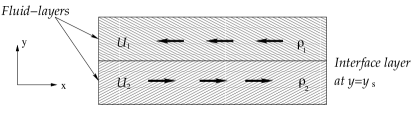
To derive the growth rate of the KHI in two dimensions including viscosity, we follow the analysis of Chandrasekhar (1961) (for a related analysis see also Funada & Joseph, 2001 and Kaiser et al., 2005). The fluid system is assumed to be viscous and incompressible. We use Cartesian coordinates in and , with two fluids at densities , , and velocities , moving anti-parallel along the -axis, separated by an interface layer at (see Fig. 1). We neglect the effect of self-gravity. The hydrodynamical equations for such a system are then given by the continuity equation
| (1) |
and the momentum equation
| (2) |
with the flow density , velocity , the thermal pressure and the kinematic viscosity .
2.1 Linear Perturbations
We linearize equations 1, and 2 with the perturbations
| (3) | |||||
| (4) | |||||
| (5) |
, express the perturbation in the velocity, and in the density and pressure, respectively. This yields the system of linearized equations as
| (6) | |||||
| (7) | |||||
| (8) | |||||
| (9) | |||||
| (10) |
Eqs. 6 and 7 represent the linearized Navier-Stokes equations, where the density may change discontinuously at the interface positions denoted by . Eq. 8 is the linearized continuity equation. In Eq. 9 the subscript distinguishes the value of the quantity at (the interface layer). The last equation, Eq. 10 expresses the incompressibility of the fluid. With perturbations of the form
| (11) |
and assuming that the flow is aligned with the perturbation vector, i.e. , we arrive at
| (12) |
where . The term, in Eq. 2.1 can be replaced with
| (13) |
The boundary condition at is determined by an integration over an infinitesimal element (), for the limit . Please note, that with Eq. 8 it follows for ,
| (14) |
After integration, the boundary condition becomes,
| (15) |
where is specifying the jump of any continuous quantity at ,
| (16) |
For we retrieve the corresponding expression as given by Chandrasekhar (1961).
2.2 Special case: constant velocities and densities
To simplify the derivation of the growth rate further, we consider the case of two fluid layers with constant densities and , and constant flow velocities and . In each region of constant and , Eq. 2.1 reduces to,
| (17) |
The layers are separated at , and must be continuous at the interface. Also, must be finite for , so that the solution of Eq. 2.2 has the following form,
| (18) | |||||
| (19) |
We assume that (which is the case if we consider two media with the same viscous properties). Inserting this in Eq. 2.1, the characteristic equation yields,
| (20) | |||
| (21) |
The parameters , are defined by,
| (22) |
| physical parameters | dimensionless | in cgs units |
|---|---|---|
| Box size | 2 | 2 cm |
| Mass | 4 | 2780.81 g |
| velocity | 0.387 | 0.40 km/s |
| time | 1 | 9.8 s |
Solving for n, we get the expression for the mode of the linear KHI:
| (23) |
applying leads to
| (24) | |||||
The mode is exponentially growing/decaying with time, if the square root of becomes imaginary,
| (25) | |||||
The first term describes oscillations (which is not of interest for the growth), the second term the growth/decay, with a damping due to the viscosity. We use this formula for the comparison with our numerical studies for different density shearing layers. For equal density shearing layers , Eq. 25 leads to
| (26) |
In § 4 and § 5 we use the velocity in direction of the perturbation, which in the above analysis refers to the -direction and therefore, to the -velocity component () when comparing with simulations. The exponential term in Eq. 11 () describes the time evolution of the KHI. In the following, we therefore compare with the analytical expectation .
3 KHI - numerical description
We use two independent numerical approaches - particle based and grid based - to follow the hydrodynamics of the system. In the following, all physical parameters are given in code units (see table 1 for conversion to physical units).
3.1 SPH models - VINE & P08
The parallel Tree-SPH code VINE (Wetzstein et al., 2009; Nelson et al., 2009) has been successfully applied to a number of astrophysical problems on various scales (Naab et al., 2006; Jesseit et al., 2007; Gritschneder et al., 2009; Walch et al., 2010; Kotarba et al., 2009). In VINE the implementation of AV is based on the description by Monaghan & Gingold (1983), and it includes the modifications by Lattanzio et al. (1986). AV is not a real physical viscosity, but implemented to allow the treatment of shock phenomena. A viscous term,
| (27) |
is added to the SPH momentum equations. The quantity prevents a singularity if , while present the mean smoothing length between two particles. For follows,
| (28) |
, and are the mean density and the mean sound
speed, respectively.
The AV-parameter controls the shear and the bulk
viscosity, whereas the parameter regulates the shock-capturing
mechanism.
In the following we set , and if not otherwise specified.
AV reduces the Reynolds-number of the flow,
resulting in the damping of the KHI (Monaghan, 2005).
Balsara (1995) proposed a corrective term, improving the behavior of the AV in shear flows.
Further improvements are discussed in Monaghan (2005)
and references therein.
VINE can be run with and without the ’Balsara-viscosity’.
To prevent the so-called ’artificial pairing’ in SPH (e.g. Schuessler &
Schmitt, 1981), we implement a
correction developed by Thomas &
Couchman (1992).
Details can be found in Wetzstein et al. (2009) and Nelson
et al. (2009).
The SPH code presented in P08 uses a different implementation of AV as
explained in Morris (1997) to prevent the side effects of artificial dissipation.
Additionally, a diffusion term called ’artificial thermal conductivity’ is implemented (see § 4.2), which
has been shown to prevent the KHI suppression in shear flows with large density
contrasts (Price, 2008).
3.2 Grid-based models - FLASH & PLUTO
We choose the publicly available, MPI-parallel FLASH code version 2.5
(Fryxell
et al., 2000). FLASH is based on the block-structured AMR technique implemented in
the PARAMESH library (MacNeice et al., 2000).
However, we do not make use of the AMR refinement technique, but use
uniform grids throughout this paper.
In FLASH’s hydrodynamic module the Navier-Stokes equations are solved
using the piecewise parabolic method (Colella &
Woodward, 1984), which incorporates a Riemann solver to compute fluxes between
individual cells.
We use a Riemann tolerance value of and a CFL of .
Due to FLASH’s hydrodynamic scheme, the intrinsic numerical viscosity
is reduced to a minimum.
This allows us to study the influence of a physical viscosity on the
growth of the KHI.
We therefore modify the hydrodynamical equations based on the
FLASH module ’diffuse’ to explicitly include a viscous term, which
scales
with a given kinematic viscosity (see 5.1 and 5.2).
As an additional test, we apply
the Godunov-type high resolution shock capturing scheme PLUTO
(Mignone et al., 2007). It is a multiphysics, multialgorithm modular
code, especially designed for the treatment of discontinuities. For
the simulations described in this paper, we employ different
Riemann-solvers and time-stepping methods on a uniform, static grid.
3.3 Initial conditions and analysis method
Our numerical ICs are identical to the ones used for the derivation of the analytical growth rates (see §2, Fig. 1 and table 1). To excite the instability, we apply a velocity perturbation in direction:
| (29) |
where is the wavenumber and is the perturbation amplitude of the -velocity triggering the
instability. The parameter controls how quickly the perturbation decreases with
(see discussion Appendix A).
It is set to if not otherwise specified.
Initial pressure and density are set to and , resulting in a
sound speed of with an adiabatic exponent of .
Since the analysis of §2 is only valid for an incompressible
fluid, the flow speed must be subsonic. We chose , and the initial perturbation is .
We tested the assumption of incompressibility by calculating , which vanishes
for incompressible flows.
This is satisfied in the linear regime, the primary focus of our work.
The wavenumber is equal to , where is the box length.
The simulated box ranges from in both directions. We use
periodic boundary conditions. If not otherwise specified the AV
parameters are set to and .
To analyze the SPH and grid simulations consistently, we
bin the SPH particles on a grid, using the cloud-in-cell method
(Hockney &
Eastwood, 1988).
For the grid codes, the same initial conditions are used. A resolution
of is adopted during the calculation, but we rebin to a
grid for the analysis.
We measure the fastest-growing mode, which is
the mode of the velocity perturbation in
direction via a Fourier analysis. For more information see
Appendix B.
We perform two sets of simulations with (i) equal
density layers (see § 4.1 for SPH and
§ 5.1 for grid codes) and (ii) unequal density layers
(see § 4.2 for SPH and § 5.2 for
grid codes). In the latter case we assume pressure equilibrium. For
SPH, we investigate the effects of equal mass and different mass
particles (see § 4.2).


4 SPH-Simulations of the KHI
In the following, we model the evolution of the KHI in systems with (§4.1) and (§4.2). We apply VINE, if not otherwise specified, and use the analytical growth rates (Eqs. 25, and 26) derived in § 2 to determine the effect of AV.
4.1 Fluid layers with equal densities:
In the case of we vary the following parameters: the resolution, which can be either enhanced by using more particles, or decreasing the smoothing length , and the AV-parameters and . We vary one parameter at a time, while the other ones are set to the fiducial values (see 3.1). In the context of AV we discuss the importance of the Balsara-viscosity. In Appendix A we also discuss the influence of different , which determines the strength of the initial vy-perturbation (Eq. 29).
-
•
Dependence on resolution:
According to the smoothing procedure in the SPH scheme, each particle requires a certain number of neighboring particles for the calculation of its physical quantities. In VINE, these range from to . The corresponding mean value of neighbors, , determines the smoothing length . For a constant particle number, increasing leads to a larger smoothing length, while at the same time the effective resolution is decreased.
In Fig. 2 we show the time evolution of the -amplitude, which describes the growth of the KHI. For the amplitudes decrease since the SPH particles lose kinetic energy by moving along the -direction into the area of the opposite stream (see Appendix A). Therefore we only consider when fitting the growth rates of the KHI. The left panel of Fig. 2 shows the amplitude growth for , , and , respectively. (The commonly used value in two dimensions is ). All three cases appear to be similar. Thus, different do not have a substantial impact on the KHI-amplitude growth.
The right panel of Fig. 2 shows the dependence on particle number, for the fiducial case of (dotted line) and for an increased resolution of (solid line). The difference for the fitted viscosity is small ().


-
•
Dependence of KHI on , :
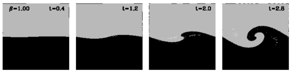
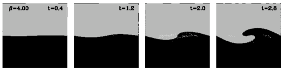
In Fig. 3, Fig. 4 and Fig. 5 we show the KHI-evolution for different values of and without the Balsara-viscosity. Increasing the AV-parameter or results in a successive suppression of the KHI. Values of and lead to a decay of the initial perturbation. However, does not affect the growth as much as . Therefore, we first concentrate on as the operating term on the KHI.
Can we assign an equivalent physical viscosity to the SPH scheme, i.e. can we determine how ”viscous” the fluid described by SPH is intrinsically? To quantify its value, the analytical slope (Eq. 26), with the viscosity being the free parameter, is fitted to the simulated growing amplitudes. We show the best fits for and in the left panel of Fig. 5, for which we find the intrinsic viscosity of and . Here we assumed the time range of , for which we determine the fits, to be well in the linear regime.
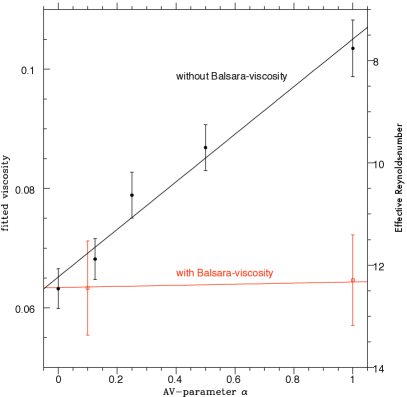
In Fig. 6 we present the derived values of as a function of . In summary, increases linearly with increasing plotted box size is from in both directions, the resolution is . , and the corresponding slope is . We also derive an offset of , which is the remaining intrinsic viscosity for . For each simulation, we also show the effective Re number of the flow (see Fig. 6, right y-axis), which was computed from . The parameter describes the characteristic scale of the perturbation, in our case the wavelength and is the velocity of the flow. Clearly, the Reynolds-numbers we reach with our models are well below the commonly expected numbers for turbulent flows ().
The effective viscosity of the flow is also influenced by different values of . Changing by a factor of two (e.g. from to ) results in an increase in effective viscosity by a factor of (see right panel of Fig. 5). -
•
Dependence on the Balsara-viscosity:
We showed that AV leads to artificial viscous dissipation, resulting in the damping of the KHI. To prevent this, we use the Balsara-viscosity, see also section 3.1. In Fig. 7 we show the corresponding amplitudes for three examples of AVs: (, ), (, ) and (, ). Clearly, the Balsara viscosity reduces the damping of the KHI, rendering almost independently of and (see also Fig. 6).

4.2 Fluid layers with variable densities:
While the previously addressed case of equal densities helped us to understand the
detailed evolution of the KHI as modeled with SPH, the astrophysically more interesting
case are shear flows with different densities.
The resolution of the diffuse region is lower by a factor of
, where is the ratio of the densities in dense and
diffuse medium (e.g. corresponds to a density contrast of ).
We return to our standard set of parameters, in which case
and .
For these low AV parameters we do not need the Balsara-viscosity (see
4.1).
(Nonetheless, we did run test simulations with the Balsara switch,
which we found to confirm our
former finding, since the growth of the KHI was not affected).
In the following, we (i) analyze the growth of the KHI for different
values of DC (with equal mass particles) and address the problem
of KHI suppression, while in (ii) we test the influence of equal mass or spatial
resolution.
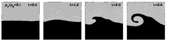
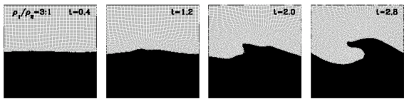
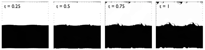
(i) KHI growth as a function of :
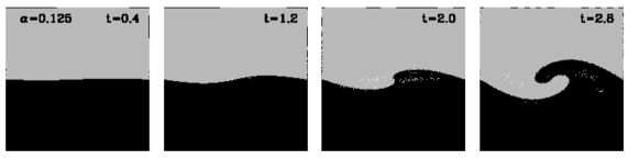
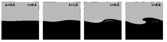
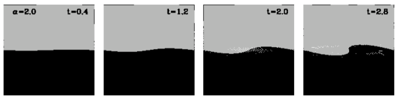
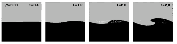
We show the KHI evolution for increasing in
Fig. 8.
For the KHI does not develop anymore.
This SPH problem of KHI suppression has been
studied in great detail (e.g. Agertz et al., 2007; Price, 2008; Wadsley et al., 2008; Read
et al., 2009; Abel, 2010).
SPH particles located at the
interface have neighbors at both sides of the
boundary (i.e. from the dense- and less dense region). Therefore, the
density at the boundary is smoothed during the evolution. However,
the corresponding entropy (or, depending on the specific code, the
thermal energy) is artificially fixed in these (isothermal) setups
which results in an artificial contribution to the SPH pressure force term, due to which the two
layers are driven apart.
One possible solution is to either adjust the density (Ritchie &
Thomas, 2001; Read
et al., 2009), or to
smooth the entropy (thermal energy)
(Price, 2008; Wadsley et al., 2008; Abel, 2010).
A remedy has been discussed by Price (2008), who proposed to add
a diffusion term, which is called artificial thermal conductivity (ATC),
to adjust the thermal energy. (For a detailed study of ATC see Price, 2008).
With this method, the KHI should develop according to the test cases of P08.
In Fig. 9 we test whether the P08 approach is
indeed in agreement with our analytical prediction. Note that P08 has a method
implemented to account for the artificial viscous dissipation
caused by AV (similar to the Balsara-viscosity). Thus, the viscous effects of AV are strongly reduced.
For and using particles in the dense layer we indeed find good
agreement between measured and analytical growth rates. If
the standard SPH scheme is used, a correction term like ATC has to be
included to obtain a KHI in shear flows with different
densities, which is consistent with the analytical prediction.
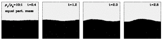
(ii) KHI growth using equal and different particle masses:
First, we investigate the development of the KHI for the standard SPH
case of equal mass resolution throughout
the computational domain, and therefore fewer particles in the low
density fluid layer (see top panel of Fig. 10 for
, where the dense medium is resolved with particles).
This results in a varying spatial resolution, due to the fact that
SPH derives the hydrodynamic quantities within a smoothing length set by
a fixed number of nearest neighbors. This construct –
as has been discussed in detail earlier in e.g. Agertz et al. 2007 –
specifically lowers the Reynolds-number of the shear flow across density
discontinuities, thus affecting the evolution of the KHI.
As can be seen in the top panel of Fig. 10, the KHI
is completely suppressed.
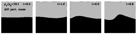
Second, we test the case of equal spatial resolution in both fluid
layers, and therefore unequal particle masses within the
computational domain (Fig. 10, lower panel).
Again, we find the KHI to grow too slowly with respect to the
analytical estimate. However, the suppression is less effectively in the latter case.
5 GRID-Simulations of the KHI
For comparison to the SPH treatment of Kelvin-Helmholtz instabilities, we study an identical setup of fluid layers with the grid-based codes FLASH and PLUTO (see §3.2). We reuse the previously specified initial conditions with a grid resolution of cells in the standard case. For FLASH, we additionally include physical viscosity of various strenghth in some of the simulations (see §3.2). Note, that for the following examples we use if not otherwise specified, which does not affect the growth of the amplitudes in the linear regime (for further information see discussion in the Appendix A).
5.1 Fluid layers with equal densities
5.1.1 Non-viscous evolution


The left panel of Fig. 11 shows the non-viscous KHI-evolution, using FLASH (solid line), PLUTO (dotted line), and for comparison VINE (dashed line). In the VINE example, the AV has been set to zero (). The expected analytical growth (Eq. 26) reduces with to (indicated by the thick dashed dotted line). The FLASH and PLUTO amplitudes develop in a similar pattern and are almost undistinguishable. Their fitted slopes within the linear regime (which lies roughly between ) results in . FLASH and PLUTO show a consistent growth in agreement with the analytical prediction. VINE on the other hand exhibits a slightly slower growth. This deviation is due to the intrinsic viscosity () that was estimated in 4.1.
5.1.2 Viscous evolution
The right panel of Fig. 11 shows the
viscous KHI-amplitudes using FLASH.
The corresponding analytical predictions (Eq. 26) are shown by
the thick dashed-dotted lines for the examples with and .
To quantify the growth of the KHI in the FLASH simulations,
we again fit the slopes of the KHI-amplitude in the linear regime
(between ). The result along with the corresponding error is plotted in
Fig. 12.
For small viscosities (), we find the growth rates of the KHI in FLASH to
be in good agreement with the analytical prediction.
In this viscosity range, the dominant term in the analytical prediction (Eq. 26) is .
Therefore, any influence of is marginal, and the amplitudes do
not change considerably. FLASH treats the fluid as if .
However, with increasing viscosity, the amplitudes should be damped.
This behavior is in fact visible in the right panel of
Fig. 11
(as well as in Fig. 12). The growth rates of the KHI
agree very well with the analytical prediction.


5.2 Fluid layers with different densities
5.2.1 Non-viscous evolution
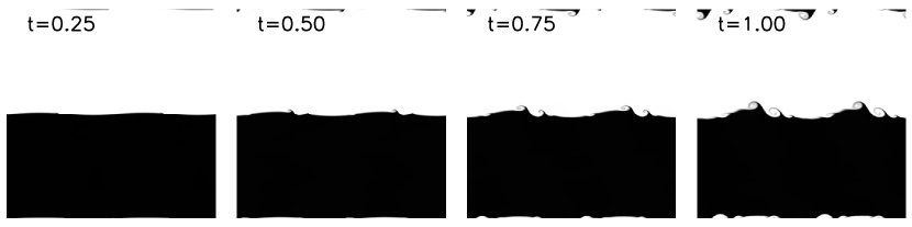
Finally, we investigate a density contrast of , similar to the
example studied with VINE (see § 4.2).
Fig. 13 shows the non-viscous evolution of the KHI
for the case (upper line for FLASH, bottom line for PLUTO).
It can be seen that for both codes the interface layer starts to roll-up and the instability
is developed. This is in disagreement with the previously discussed case using SPH, where the KHI is completely
suppressed for DC (see 4.2).
The left panel of Fig. 14 presents the corresponding
amplitudes for FLASH (solid line) and PLUTO (dotted line) compared to the analytical
prediction (thick dashed-dotted line), which in this case reduces to
| (30) |
For FLASH we show two different resolutions ( and ).
The amplitudes resulting in the case of low and high resolution are effectively indistinguishable.
This is an important result, as it demonstrates that small scale
perturbations, which arise due to numerical noise and which could
violate the linear analysis (as we then might follow the
growth of higher order modes rather than the initial perturbation) are
not important. Therefore, we have shown that our simulations are
converged as we would otherwise expect the growth of the KHI to be slightly dependent on the
grid resolution (see e.g. the recent findings of Robertson et al. (2010), who had to
smooth the density gradient between the two fluid layers in order
to achieve convergence in terms of grid resolution).
Moreover, both FLASH and PLUTO evolve similarly. For all three
examples the slope of the amplitude evolution can be approximated to
, which is in good agreement with the analytical expectation.
Note that we do not show the comparison with the VINE amplitude since the KHI
does not evolve for (see 4.2).
Many grid codes offer a variety of hydrodynamical solvers. We
therefore tested the influence of different numerical schemes on
the growth of the KHI using PLUTO (see right panel of
Fig. 14 ).
We show three different examples; ’sim000’ is a Lax-Friedrichs scheme
together with a second order Runge-Kutta solver (tvdlf); ’sim001’
implements a two-shock Riemann solver with linear reconstruction
embedded in a second order Runge-Kutta scheme;
’sim002’ also implements a two-shock Riemann solver, but with
parabolic reconstruction, and embedded in a third order Runge-Kutta
scheme. Both, ’sim001’ and ’sim002’ show a similar growth of the KHI
in agreement with the analytical prediction (see
Fig. 14, top right panel). The more
diffusive scheme used in ’sim000’ causes a small delay in the growth
of the KHI, but results in a similar slope within the linear regime (up to ).
5.2.2 Viscous evolution
Fig. 15 shows the viscous KHI-amplitudes using FLASH, which are increasingly suppressed with . The corresponding analytical prediction (Eq. 25) is shown for , and (thick dashed-dotted lines). For the simulated growth rate is slightly enhanced by a factor of as compared to the analytical prediction (see also Fig. 12). However, for higher viscosities () we find good agreement between simulation and analytical prediction.
6 Conclusions
We have studied the Kelvin-Helmholtz instability applying different numerical schemes.
We use two methods for our SPH models, namely the
Tree-SPH code VINE (Wetzstein et al., 2009; Nelson
et al., 2009),
and the code developed by Price (2008).
The grid based simulations of the KHI rely on FLASH
(Fryxell
et al., 2000), while as a test for the non-viscous evolution we
also apply PLUTO (Mignone et al., 2007).
We first extended the analytical prescription of the KHI by
Chandrasekhar (1961) to include a constant viscosity. With this
improvement we were able to measure the intrinsic viscosity of our
subsequently performed numerical simulations. We test both SPH as well
as grid codes with this method.
We then concentrated on the KHI-evolution with SPH.
We performed a resolution study to measure the dependence of
the KHI growth on the mean number of SPH neighbors () and the total
number of particles, respectively. We found that our simulations were
well resolved and that a different number of
did not significantly influence the KHI growth rate.
In case of equal density shearing layers we then measured the
intrinsic viscosity in VINE by evaluating our simulations against the analytical prediction in the linear regime.
Without using the Balsara viscosity the AV parameters and effectively lead to a damping of the KHI.
The commonly suggested and used settings of , and
result in a strong suppression of the KHI.
More quantitatively, we derive values of for .
Different values of do not have a strong impact on
.
By introducing the Balsara-viscosity the dissipative effects of the AV
can be reduced significantly, effectively rendering the results to be
independent of and . However, the constant floor viscosity of prevails.
Furthermore for a given , we estimated the effective
Reynolds-number () of the flow.
For the minimum SPH viscosity of
we derive a maximum Reynolds number of .
This is very small compared to typical Reynolds numbers of real turbulent flows ().
For different density shearing layers we confirmed the results
discussed in Agertz et al. (2007), i.e. the KHI is completely
suppressed for shear flows with different densities (in the case of
VINE for ).
Here, using the Balsara switch does not solve the problem. This
indicates that other changes to the SPH formalism are required in
order to correctly model shearing layers of different densities. To demonstrate this we applied the
solution of Price (2008)
to our initial conditions for DC=10. In this case the KHI was
suppressed in VINE. However, we found good agreement between the
analytically predicted amplitude evolution and the simulation of
Price (2008) for .
The second part of this paper addresses the non-viscous- and viscous KHI
evolution using grid codes.
In the case of equal density shearing layers, we found the non-viscous growth rates
for shear flows with FLASH and PLUTO to be in good agreement with the analytical prediction.
In the viscous case, the FLASH-amplitudes show only a minor dependency on the
viscosity if .
Increasing the viscosity leads to a damped evolution, with the simulated
growth coinciding with the analytical prediction.
For non-viscous shear flows (with a density contrast of ) the
KHI does develop for FLASH and PLUTO in agreement with the analytical
prediction. In the viscous case FLASH (also analyzed with )
slightly overpredicts the
corresponding growth rates for by a constant factor of
.
The comparison between VINE, FLASH and PLUTO in the equal density case, where and , demonstrated that VINE does
have an intrinsic viscosity (which we estimated to ).
Acknowledgments
I would like to thank Volker Springel for his useful suggestions, and Thorsten Naab for his support. Many thanks also to Oscar Agertz for helpful discussions, as well as Eva Ntormousi. This research was supported by the DFG priority program SPP 1177 and by the DFG cluster of excellence ’Origin and Structure of the Universe’. Part of the simulations were run on the local SGI ALTIX 3700 Bx2 which was also partly funded by this cluster of excellence. FLASH was developed by the DOE-supported ASC/Alliance Center for Astrophysical Thermonuclear Flashes at the University of Chicago. S.Walch gratefully acknowledges the support of the EC-funded Marie Curie Research Training Network Constellation (MRTN-CT-2006-035890). M. Wetzstein gratefully acknowledges support from NSF grant 0707731.
References
- Abel (2010) Abel T., 2010, ArXiv e-prints
- Agertz et al. (2007) Agertz O., Moore B., Stadel J., Potter D., Miniati F., Read J., Mayer L., Gawryszczak A., Kravtsov A., Nordlund Å., Pearce F., Quilis V., Rudd D., Springel V., Stone J., Tasker E., Teyssier R., Wadsley J., Walder R., 2007, MNRAS, 380, 963
- Agertz et al. (2009) Agertz O., Teyssier R., Moore B., 2009, MNRAS, 397, L64
- Balsara (1995) Balsara D. S., 1995, Journal of Computational Physics, 121, 357
- Banerjee et al. (2007) Banerjee R., Klessen R. S., Fendt C., 2007, ApJ, 668, 1028
- Benz (1990) Benz W., 1990, in Buchler J. R., ed., Numerical Modelling of Nonlinear Stellar Pulsations Problems and Prospects Smooth Particle Hydrodynamics - a Review. pp 269–+
- Bland-Hawthorn et al. (2007) Bland-Hawthorn J., Sutherland R., Agertz O., Moore B., 2007, ApJL, 670, L109
- Burkert (2006) Burkert A., 2006, Comptes Rendus Physique, 7, 433
- Burkert et al. (2008) Burkert A., Naab T., Johansson P. H., Jesseit R., 2008, ApJ, 685, 897
- Carroll et al. (2009) Carroll J. J., Frank A., Blackman E. G., Cunningham A. J., Quillen A. C., 2009, ApJ, 695, 1376
- Chandrasekhar (1961) Chandrasekhar S., 1961, Hydrodynamic and Hydromagnetic Stability. Dover Publications
- Colagrossi (2004) Colagrossi A., 2004, Dottorato di Ricerca in Meccanica Teorica ed Applicata XVI CICLO, A meshless Lagrangian method for free-surface and interface flows with fragmentation, Phd Thesis. Universita di Roma, La Sapienza
- Colella & Woodward (1984) Colella P., Woodward P. R., 1984, Journal of Computational Physics, 54, 174
- Couchman et al. (1995) Couchman H. M. P., Thomas P. A., Pearce F. R., 1995, ApJ, 452, 797
- Das & Chattopadhyay (2008) Das S., Chattopadhyay I., 2008, New Astronomy, 13, 549
- Dekel et al. (2009) Dekel A., Birnboim Y., Engel G., Freundlich J., Goerdt T., Mumcuoglu M., Neistein E., Pichon C., Teyssier R., Zinger E., 2009, Nature, 457, 451
- Diemand et al. (2008) Diemand J., Kuhlen M., Madau P., Zemp M., Moore B., Potter D., Stadel J., 2008, Nature, 454, 735
- Español & Revenga (2003) Español P., Revenga M., 2003, Phys. Rev. E, 67, 026705
- Evrard et al. (1994) Evrard A. E., Summers F. J., Davis M., 1994, ApJ, 422, 11
- Flebbe et al. (1994) Flebbe O., Muenzel S., Herold H., Riffert H., Ruder H., 1994, ApJ, 431, 754
- Fryxell et al. (2000) Fryxell B., Olson K., Ricker P., Timmes F. X., Zingale M., Lamb D. Q., MacNeice P., Rosner R., Truran J. W., Tufo H., 2000, ApJS, 131, 273
- Funada & Joseph (2001) Funada T., Joseph D. D., 2001, Journal of Fluid Mechanics, 445, 263
- Gingold & Monaghan (1977) Gingold R. A., Monaghan J. J., 1977, MNRAS, 181, 375
- Gritschneder et al. (2009) Gritschneder M., Naab T., Burkert A., Walch S., Heitsch F., Wetzstein M., 2009, MNRAS, 393, 21
- Gritschneder et al. (2009) Gritschneder M., Naab T., Walch S., Burkert A., Heitsch F., 2009, ApJL, 694, L26
- Heinzeller et al. (2009) Heinzeller D., Duschl W. J., Mineshige S., 2009, MNRAS, 397, 890
- Heitsch & Putman (2009) Heitsch F., Putman M. E., 2009, ApJ, 698, 1485
- Hernquist & Katz (1989) Hernquist L., Katz N., 1989, ApJS, 70, 419
- Hockney & Eastwood (1988) Hockney R. W., Eastwood J. W., 1988, Computer simulation using particles. Institute of Physics Publishing
- Jesseit et al. (2007) Jesseit R., Naab T., Peletier R. F., Burkert A., 2007, MNRAS, 376, 997
- Kaiser et al. (2005) Kaiser C. R., Pavlovski G., Pope E. C. D., Fangohr H., 2005, MNRAS, 359, 493
- Katz et al. (1992) Katz N., Hernquist L., Weinberg D. H., 1992, ApJL, 399, L109
- Kotarba et al. (2009) Kotarba H., Lesch H., Dolag K., Naab T., Johansson P. H., Stasyszyn F. A., 2009, MNRAS, 397, 733
- Lanzafame et al. (2006) Lanzafame G., Belvedere G., Molteni D., 2006, AAP, 453, 1027
- Lattanzio et al. (1986) Lattanzio J., Monaghan J., Pongracic H., Schwartz M., 1986, SIAM Journal on Scientific and Statistical Computing, 7, 591
- Lucy (1977) Lucy L. B., 1977, AJ, 82, 1013
- MacNeice et al. (2000) MacNeice P., Olson K. M., Mobarry C., de Fainchtein R., Packer C., 2000, Computer Physics Communications, 126, 330
- Marri & White (2003) Marri S., White S. D. M., 2003, MNRAS, 345, 561
- Mignone et al. (2007) Mignone A., Bodo G., Massaglia S., Matsakos T., Tesileanu O., Zanni C., Ferrari A., 2007, ApJS, 170, 228
- Monaghan (1992) Monaghan J. J., 1992, ARA& A, 30, 543
- Monaghan (2005) Monaghan J. J., 2005, Reports of Progress in Physics, 68, 1703
- Monaghan & Gingold (1983) Monaghan J. J., Gingold R. A., 1983, Journal of Computational Physics, 52, 374
- Morris (1997) Morris J., 1997, Journal of Computational Physics, 136, 41
- Murray et al. (1993) Murray S. D., White S. D. M., Blondin J. M., Lin D. N. C., 1993, ApJ, 407, 588
- Naab et al. (2006) Naab T., Jesseit R., Burkert A., 2006, MNRAS, 372, 839
- Navarro et al. (1995) Navarro J. F., Frenk C. S., White S. D. M., 1995, MNRAS, 275, 56
- Nelson et al. (2009) Nelson A. F., Wetzstein M., Naab T., 2009, ApJS, 184, 326
- Park (2009) Park M., 2009, ApJ, 706, 637
- Price (2008) Price D. J., 2008, Journal of Computational Physics, 227, 10040
- Quilis & Moore (2001) Quilis V., Moore B., 2001, ApJL, 555, L95
- Read et al. (2009) Read J. I., Hayfield T., Agertz O., 2009, ArXiv 0906.0774
- Ritchie & Thomas (2001) Ritchie B. W., Thomas P. A., 2001, MNRAS, 323, 743
- Robertson et al. (2010) Robertson B. E., Kravtsov A. V., Gnedin N. Y., Abel T., Rudd D. H., 2010, MNRAS, 401, 2463
- Schuessler & Schmitt (1981) Schuessler I., Schmitt D., 1981, AAP, 97, 373
- Serna et al. (2003) Serna A., Domínguez-Tenreiro R., Sáiz A., 2003, ApJ, 597, 878
- Sijacki & Springel (2006) Sijacki D., Springel V., 2006, MNRAS, 371, 1025
- Springel (2010) Springel V., 2010, MNRAS, 401, 791
- Springel & Hernquist (2002) Springel V., Hernquist L., 2002, MNRAS, 333, 649
- Steinmetz & Navarro (1999) Steinmetz M., Navarro J. F., 1999, ApJ, 513, 555
- Steinmetz & Navarro (2002) Steinmetz M., Navarro J. F., 2002, New Astronomy, 7, 155
- Takeda et al. (1994) Takeda H., Miyama S. M., Sekiya M., 1994, Progress of Theoretical Physics, 92, 939
- Thacker & Couchman (2000) Thacker R. J., Couchman H. M. P., 2000, ApJ, 545, 728
- Thacker et al. (2000) Thacker R. J., Tittley E. R., Pearce F. R., Couchman H. M. P., Thomas P. A., 2000, MNRAS, 319, 619
- Thomas & Couchman (1992) Thomas P. A., Couchman H. M. P., 1992, MNRAS, 257, 11
- Vietri et al. (1997) Vietri M., Ferrara A., Miniati F., 1997, ApJ, 483, 262
- Wadsley et al. (2008) Wadsley J. W., Veeravalli G., Couchman H. M. P., 2008, MNRAS, 387, 427
- Walch et al. (2010) Walch S., Naab T., Whitworth A., Burkert A., Gritschneder M., 2010, MNRAS, 402, 2253
- Wetzstein et al. (2009) Wetzstein M., Nelson A. F., Naab T., Burkert A., 2009, ApJS, 184, 298
Appendix A Dependence of KHI-amplitudes on


Dependence of KHI on :
This parameter determines the strength of the initial
-perturbation (Eq. 29).
In Fig. 2
we show the time evolution of the vy-amplitude, which describes the
growth of the KHI. For the amplitudes decrease since the
SPH particles lose kinetic energy by moving along the y-direction into the area of the opposite stream.
If the magnitude of the initial perturbation is low (i.e. small
), then the decrease in the amplitude is stronger than for
e.g. , where the initial perturbation is large and
the decrease less prominent. But independently of the value
of the subsequent growth of the instability is similar, and we obtain
comparable results neglecting the decreasing initial part.
Fig. 16 shows the dependency of the KHI-amplitudes using different values of , for VINE (left side) and
FLASH (right side). For this example we use equal density layers, where for FLASH a viscosity of has been taken.
Clearly visible is the initial drop caused by a low value of . This is the case for both codes, and arises
due to the transformation of energy to build up the KHI. The
fitted slopes do not vary much with . To extract the slopes,
we concentrate on the time evolution after this initial drop.
Appendix B Measuring the KHI-amplitudes

To measure the amplitude growth of the KHI, we apply a Fourier-Transformation (FT) to
the -velocity component of the grid points. The FT allows to select the desired modes
reducing the numerical noise.
The region of our focus, and contains one
mode of the -perturbation (Eq. 29) triggering the instability, see Fig. 17.
The shaded regions comprise the particles subject to the FT (at
and ).
The maximum of the FT gives the dominant mode and its
corresponding velocity amplitude, which we compare with the analytical
model.