Fourier Theory on the Complex Plane III
Low-Pass Filters, Singularity Splitting
and Infinite-Order Filters

Abstract

When Fourier series are employed to solve partial differential equations, low-pass filters can be used to regularize divergent series that may appear. In this paper we show that the linear low-pass filters defined in a previous paper can be interpreted in terms of the correspondence between Fourier Conjugate (FC) pairs of Definite Parity (DP) Fourier series and inner analytic functions, which was established in earlier papers. The action of the first-order linear low-pass filter corresponds to an operation in the complex plane that we refer to as “singularity splitting”, in which any given singularity of an inner analytic function on the unit circle is replaced by two softer singularities on that same circle, thus leading to corresponding DP Fourier series with better convergence characteristics. Higher-order linear low-pass filters can be easily defined within the unit disk of the complex plane, in terms of the first-order one. The construction of infinite-order filters, which always result in $C^{\infty}$ real functions over the unit circle, and in corresponding DP Fourier series which are absolutely and uniformly convergent to these functions, is presented and discussed.

1 Introduction

In a previous paper [1] a one-to-one correspondence between FC (Fourier Conjugate) pairs of DP (Definite Parity) Fourier series and inner analytic functions on the open unit disk was established. In a subsequent paper [2] the questions related to the convergence of such series were examined in the light of this correspondence. In those papers certain techniques were presented for the recovery of the real functions from the coefficients of their DP Fourier series, which work even if the series are divergent. This included a technique we called “singularity factorization” that from the (possibly divergent) DP Fourier series of a given real function leads to certain expressions involving alternative trigonometric series, with better convergence characteristics, that converge to that same real function. The reader is referred to those papers for many of the concepts and notations used in this paper.

In another previous paper [3] certain low-pass filters acting in the space of integrable real functions were introduced, and their use for the regularization of divergent Fourier series in boundary value problems was discussed. In the present paper we will show that these low-pass filters can be interpreted and realized within the open unit disk of the complex plane in a very simple way, in the context of the correspondence between FC pairs of DP Fourier series and inner analytic functions within that disk, which was discussed in the aforementioned earlier papers [1] and [2]. In line with our discussion in those papers, about ways of recovering the real functions from their Fourier coefficients when the Fourier series do not converge, or converge poorly, here we will show that the use of low-pass filters can be interpreted as one more such technique. However, unlike the previous ones it involves a certain type of approximation, and its application changes the series and functions in a specific way, that is small in a certain sense, as described in [3]. From a purely mathematical standpoint the discussion of these filters consists of the examination of the properties of a certain set of integral operators acting in the space of integrable real functions.

Let us review briefly the facts about the filters, when defined on a periodic interval. As given in [3], the first-order linear low-pass filter is defined in the following way, if we adopt as the domain of our real functions the periodic interval $[-\pi,\pi]$. Given a real function $f(\theta)$ of the real angular variable $\theta$ in that interval, of which we require no more than that it be integrable, we define from it a filtered function $f_{\epsilon}^{(1)}(\theta)$ as

$$f_{\epsilon}^{(1)}(\theta)=\frac{1}{2\epsilon}\int_{\theta-\epsilon}^{\theta+\epsilon}d\theta^{\prime}\,f\!\left(\theta^{\prime}\right),$$ (1)

where the angular parameter $\epsilon\leq\pi$ is a strictly positive real parameter which we will refer to as the range of the filter. One can also define $f_{0}^{(1)}(\theta)$ by continuity, as the $\epsilon\to 0$ limit of this expression. The filter can be understood as a linear integral operator acting in the space of integrable real functions, as is done in [3]. It may be written as an integral over the whole periodic interval involving a kernel $K_{\epsilon}^{(1)}\!\left(\theta-\theta^{\prime}\right)$ with compact support,

$$f_{\epsilon}^{(1)}(\theta)=\int_{-\pi}^{\pi}d\theta^{\prime}\,K_{\epsilon}^{(1)}\!\left(\theta-\theta^{\prime}\right)f\!\left(\theta^{\prime}\right),$$

where the kernel is defined as $K_{\epsilon}^{(1)}\!\left(\theta-\theta^{\prime}\right)=1/(2\epsilon)$ for $\left|\theta-\theta^{\prime}\right|<\epsilon$, and as $K_{\epsilon}^{(1)}\!\left(\theta-\theta^{\prime}\right)=0$ for $\left|\theta-\theta^{\prime}\right|>\epsilon$. Since we are in the periodic interval, it should be noted that what we mean here by “compact support” is the fact that the kernel is different from zero only within an interval contained in the periodic interval. We may have at most that the two intervals coincide, with $\epsilon=\pi$, and in general we will assume that we have $\epsilon\leq\pi$. The most interesting case, however, is that in which we have $\epsilon\ll\pi$. We may say then that this kernel is a discontinuous even function of $\left(\theta-\theta^{\prime}\right)$ that has unit integral and compact support. As shown in [3], it can be expressed in terms of a point-wise convergent Fourier series,

$$K_{\epsilon}^{(1)}\!\left(\theta-\theta^{\prime}\right)=\frac{1}{2\pi}+\frac{1}{\pi}\sum_{k=1}^{\infty}\left[\frac{\sin(k\epsilon)}{(k\epsilon)}\right]\cos\!\left[k\left(\theta-\theta^{\prime}\right)\right].$$

The filter defined above has several interesting properties, which are the reasons for its usefulness, the most important and basic ones of which are listed and demonstrated in [3]. In this paper we will refer to and use these properties as the occasion arises. Also, as part of the demonstrations discussed in Section 3 we will have the opportunity to examine some more of these properties in Appendix B.

As discussed in [3], since the first-order filter defined here is a linear operator, one can construct higher-order filters by simply applying it multiple times to a given real function. This leads directly to the definition of higher-order filters, for example the second-order one, with range $2\epsilon$, and assuming that $\epsilon\leq\pi/2$,

$$f_{2\epsilon}^{(2)}(\theta)=\int_{-\infty}^{\infty}d\theta^{\prime}\,K_{2\epsilon}^{(2)}\!\left(\theta-\theta^{\prime}\right)f\!\left(\theta^{\prime}\right),$$

where, as a consequence of the definition of the first-order filter, the second-order kernel with range $2\epsilon$ is given by the application of the first-order filter to the first-order kernel,

$$K_{2\epsilon}^{(2)}\!\left(\theta-\theta^{\prime\prime}\right)=\int_{-\infty}^{\infty}d\theta^{\prime}\,K_{\epsilon}^{(1)}\!\left(\theta-\theta^{\prime}\right)K_{\epsilon}^{(1)}\!\left(\theta^{\prime}-\theta^{\prime\prime}\right).$$

This second-order kernel is a continuous but non-differentiable even function of $\left(\theta-\theta^{\prime}\right)$. Due to the properties of the first-order filter regarding its action on Fourier expansions [10, 11], the second-order kernel is also given by the absolutely and uniformly convergent Fourier series

$$K_{2\epsilon}^{(2)}\!\left(\theta-\theta^{\prime}\right)=\frac{1}{2\pi}+\frac{1}{\pi}\sum_{k=1}^{\infty}\left[\frac{\sin(k\epsilon)}{(k\epsilon)}\right]^{2}\cos\!\left[k\left(\theta-\theta^{\prime}\right)\right],$$

so long as $\epsilon\leq\pi/2$. Both the first and second-order kernels are even functions of $\left(\theta-\theta^{\prime}\right)$ with unit integral and compact support. The range of the first-order filter is given by $\epsilon$, and if one just applies the filter twice as we did here, that range doubles do $2\epsilon$. However, one may compensate for this by simply applying twice the first-order filter with parameter $\epsilon/2$, thus resulting in a second-order filter with range $\epsilon$, given by the absolutely and uniformly convergent Fourier series

$$K_{\epsilon}^{(2)}\!\left(\theta-\theta^{\prime}\right)=\frac{1}{2\pi}+\frac{1}{\pi}\sum_{k=1}^{\infty}\left[\frac{\sin(k\epsilon/2)}{(k\epsilon/2)}\right]^{2}\cos\!\left[k\left(\theta-\theta^{\prime}\right)\right],$$

so long as $\epsilon\leq\pi$. This procedure can be iterated $N$ times to produce an order-$N$ filter with range $N\epsilon$. Given the properties of the first-order filter regarding its action on Fourier expansions [10, 11], the Fourier representation of the order-$N$ kernel can easily be written explicitly,

$$K_{N\epsilon}^{(N)}\!\left(\theta-\theta^{\prime}\right)=\frac{1}{2\pi}+\frac{1}{\pi}\sum_{k=1}^{\infty}\left[\frac{\sin(k\epsilon)}{(k\epsilon)}\right]^{N}\cos\!\left[k\left(\theta-\theta^{\prime}\right)\right],$$ (2)

so long as $\epsilon\leq\pi/N$. This definition can be extended down to the case of the order-zero kernel, with $N=0$, which is simply the Dirac delta “function”, and which is in fact given, as shown in [2], by the divergent Fourier series

$$\delta\!\left(\theta-\theta^{\prime}\right) = K_{0}^{(0)}\!\left(\theta-\theta^{\prime}\right)$$

$$= \frac{1}{2\pi}+\frac{1}{\pi}\sum_{k=1}^{\infty}\cos\!\left[k\left(\theta-\theta^{\prime}\right)\right].$$

This can be understood as the kernel of an order-zero filter, which is the identity almost everywhere. If we simply exchange $\epsilon$ by $\epsilon/N$ in the expression in Equation (2) we get the order-$N$ filter with range $\epsilon$, written in terms of its Fourier expansion,

$$K_{\epsilon}^{(N)}\!\left(\theta-\theta^{\prime}\right)=\frac{1}{2\pi}+\frac{1}{\pi}\sum_{k=1}^{\infty}\left[\frac{\sin(k\epsilon/N)}{(k\epsilon/N)}\right]^{N}\cos\!\left[k\left(\theta-\theta^{\prime}\right)\right],$$

so long as $\epsilon\leq\pi$. Note that this series converges ever faster as $N$ increases, and that it can be differentiated $N-2$ times still resulting in absolutely and uniformly convergent series, and $N-1$ times still resulting in point-wise convergent series. The series for $K_{0}^{(0)}\!\left(\theta-\theta^{\prime}\right)$ is the only one which is not convergent, and of the remaining ones that for $K_{\epsilon}^{(1)}\!\left(\theta-\theta^{\prime}\right)$ is the only one which is not absolutely or uniformly convergent, although it is point-wise convergent. For $N\geq 2$ all the Fourier series of the kernels, regardless of range, are absolutely and uniformly convergent to functions which are $C^{N-2}$ everywhere. All these kernels, regardless of order or range, are even functions of $\left(\theta-\theta^{\prime}\right)$ with unit integral and compact support, so long as $\epsilon\leq\pi$.

Therefore, one is led to think of the possibility that in the limit $N\to\infty$ this sequence of order-$N$ kernels with constant range $\epsilon$ could converge to a $C^{\infty}$ kernel function $K_{\epsilon}^{(\infty)}\!\left(\theta-\theta^{\prime}\right)$ with compact support. The corresponding infinite-order filter would then map any merely integrable function to a $C^{\infty}$ function. Although it turns out to be possible to construct a infinite-order kernel with such a property, it is not to be obtained by the limit described here, as we will see later in Section 3.

2 The Low-Pass Filter on the Complex Plane

According to the correspondence established in [1], to each FC pair of DP Fourier series corresponds an inner analytic function $w(z)$ within the open unit disk. Each operation performed on the DP Fourier series corresponds to a related operation on the inner analytic function, possibly represented by its Taylor series around the origin. For example, differentiation of the DP Fourier series with respect to their real variable $\theta$ corresponds to logarithmic differentiation of $w(z)$ with respect to $z$, as shown in [2]. If we imagine that the first-order low-pass filter is to be implemented on the DP real functions $f_{\rm c}(\theta)$ and $f_{\rm s}(\theta)$ associated to the DP Fourier series, where for $z=\rho\exp(\mbox{\boldmath$\imath$}\theta)$ and $\rho=1$ we have

$$w(z)=f_{\rm c}(\theta)+\mbox{\boldmath$\imath$}f_{\rm s}(\theta),$$

then it is clear that a corresponding filtering operation over $w(z)$ must exist within the open unit disk. In this section we will give the definition of this filtering operation on the complex plane, and derive some of its properties.

Consider then an inner analytic function $w(z)$, with $z=\rho\exp(\mbox{\boldmath$\imath$}\theta)$ and $0\leq\rho\leq 1$. We define from it the corresponding filtered complex function, using the real angular range parameter $0<\epsilon\leq\pi$, by

$$w_{\epsilon}(z)=-\,\frac{\mbox{\boldmath$\imath$}}{2\epsilon}\int_{z_{\ominus}}^{z_{\oplus}}dz^{\prime}\,\frac{1}{z^{\prime}}\,w\!\left(z^{\prime}\right),$$ (3)

involving an integral over the arc of circle illustrated in Figure 1, where the two extremes are given by

$$z_{\ominus} = z\,{\rm e}^{-\mbox{\boldmath$\imath$}\epsilon}$$

$$= \rho\,{\rm e}^{\mbox{\boldmath$\imath$}(\theta-\epsilon)},$$

$$z_{\oplus} = z\,{\rm e}^{\mbox{\boldmath$\imath$}\epsilon}$$

$$= \rho\,{\rm e}^{\mbox{\boldmath$\imath$}(\theta+\epsilon)}.$$

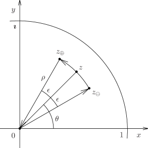
Figure 1: Illustration of the definition of the first-order linear low-pass filter within the unit disk of the complex plane. The average is taken over the arc of circle from $z_{\ominus}$ to $z_{\oplus}$.

It is important to observe that this definition can be implemented at all the points of the unit disk, with the single additional proviso that at $z=0$ the filter be defined as the identity. Note that the definition in Equation (3) has the form of a logarithmic integral, which is the inverse operation to the logarithmic derivative, as defined and discussed in [2]. What we are doing here is to map the value of the function $w(z)$ at $z$ to the average of $w(z)$ over the symmetric arc of circle of angular length $2\epsilon$ around $z$, with constant $\rho$. This defines a new complex function $w_{\epsilon}(z)$ at that point. Since on the arc of circle we have that $z^{\prime}=\rho\exp(\mbox{\boldmath$\imath$}\theta^{\prime})$ and hence that $dz^{\prime}=\mbox{\boldmath$\imath$}z^{\prime}d\theta^{\prime}$, we may also write the definition as

$$w_{\epsilon}(z)=\frac{1}{2\epsilon}\int_{\theta-\epsilon}^{\theta+\epsilon}d\theta^{\prime}\,w\!\left(\rho,\theta^{\prime}\right),$$

which makes the averaging process explicitly clear. As one might expect, just as the logarithmic differentiation of inner analytic functions corresponds to derivatives with respect to $\theta$, the logarithmic integration corresponds to integrals on $\theta$. Note that for $\epsilon=\pi$ the complex filtered function $w_{\epsilon}(z)$ is simply a constant function, possibly with removable singularities on the unit circle. Since our real functions here, being the real or imaginary parts of inner analytic functions, are zero-average functions, that constant is actually zero, for all inner analytic functions.

Let us show that $w_{\epsilon}(z)$ is an inner analytic function, as defined in [1]. Note that since $w(z)$ is an inner analytic function, it has the property that $w(0)=0$. Therefore we see that because $w(0)=0$ the integrand in Equation (3) is analytic within the open unit circle, if defined by continuity at $z=0$. Consider therefore the integral over the closed oriented circuit shown in Figure 1,

$$\int_{0}^{z_{\ominus}}dz^{\prime}\,\frac{1}{z^{\prime}}\,w\!\left(z^{\prime}\right)+\int_{z_{\ominus}}^{z_{\oplus}}dz^{\prime}\,\frac{1}{z^{\prime}}\,w\!\left(z^{\prime}\right)+\int_{z_{\oplus}}^{0}dz^{\prime}\,\frac{1}{z^{\prime}}\,w\!\left(z^{\prime}\right)=0.$$ (4)

Since the contour is closed and the integrand is analytic on it and within it, this integral is zero due to the Cauchy-Goursat theorem. It follows that we have

$$\int_{z_{\ominus}}^{z_{\oplus}}dz^{\prime}\,\frac{1}{z^{\prime}}\,w\!\left(z^{\prime}\right)=\int_{0}^{z_{\oplus}}dz^{\prime}\,\frac{1}{z^{\prime}}\,w\!\left(z^{\prime}\right)-\int_{0}^{z_{\ominus}}dz^{\prime}\,\frac{1}{z^{\prime}}\,w\!\left(z^{\prime}\right).$$

These last two integrals give the logarithmic primitive of $w(z)$ at the two ends of the arc, as defined in [2]. According to that definition the logarithmic primitive of $w(z)$ is given by

$$w^{-1\!\mbox{\Large$\cdot$}\!}(z)=\int_{0}^{z}dz^{\prime}\,\frac{1}{z^{\prime}}\,w\!\left(z^{\prime}\right),$$

where we are using the notation for the logarithmic primitive introduced in that paper. The logarithmic primitive $w^{-1\!\mbox{\Large$\cdot$}\!}(z)$ is an inner analytic function within the open unit disk, as shown in [2]. It follows that we have

$$\int_{z_{\ominus}}^{z_{\oplus}}dz^{\prime}\,\frac{1}{z^{\prime}}\,w\!\left(z^{\prime}\right)=w^{-1\!\mbox{\Large$\cdot$}\!}(z_{\oplus})-w^{-1\!\mbox{\Large$\cdot$}\!}(z_{\ominus}).$$

Since the logarithmic primitive $w^{-1\!\mbox{\Large$\cdot$}\!}(z)$ is an inner analytic function, and since the functions $z_{\ominus}(z)$ and $z_{\oplus}(z)$ are also rotated inner analytic functions, as can easily be verified, it is reasonable to think that the right-hand side of this equation is an inner analytic function. We have therefore for the filtered complex function

$$w_{\epsilon}(z)=-\,\frac{\mbox{\boldmath$\imath$}}{2\epsilon}\left[w^{-1\!\mbox{\Large$\cdot$}\!}(z_{\oplus})-w^{-1\!\mbox{\Large$\cdot$}\!}(z_{\ominus})\right],$$ (5)

which indicates that $w_{\epsilon}(z)$ is an inner analytic function as well. In fact, the analyticity of $w_{\epsilon}(z)$ is evident, since it is a linear combination of two analytic functions within the open unit disk. We must also show that $w_{\epsilon}(0)=0$ and that $w_{\epsilon}(z)$ reduces to a real function on the interval $(-1,1)$ of the real axis, which are the additional properties defining an inner analytic function, as given in [1]. It is easy to check directly that $w_{\epsilon}(0)=0$, since $w^{-1\!\mbox{\Large$\cdot$}\!}(0)=0$, given that the logarithmic primitive is an inner analytic function. In order to establish the remaining property, we replace $z$ by a real $x$ in the filtered function, and taking the complex conjugate of that function with argument $x$ we get

$$w_{\epsilon}^{*}(x)=\frac{\mbox{\boldmath$\imath$}}{2\epsilon}\left[w^{-1\!\mbox{\Large$\cdot$}\!}\!\left(x\,{\rm e}^{\mbox{\boldmath$\imath$}\epsilon}\right)-w^{-1\!\mbox{\Large$\cdot$}\!}\!\left(x\,{\rm e}^{-\mbox{\boldmath$\imath$}\epsilon}\right)\right]^{*}.$$

Now, since $w^{-1\!\mbox{\Large$\cdot$}\!}(z)$ is an inner analytic function, it follows that $w^{-1\!\mbox{\Large$\cdot$}\!}(x)$ is a real function. Therefore the only relevant participation of the number $\imath$ in the quantity within the brackets in the expression above is that introduced explicitly via the arguments. We have therefore, taking the complex conjugates on the right-hand side,

$$w_{\epsilon}^{*}(x) = \frac{\mbox{\boldmath$\imath$}}{2\epsilon}\left[w^{-1\!\mbox{\Large$\cdot$}\!}\!\left(x\,{\rm e}^{-\mbox{\boldmath$\imath$}\epsilon}\right)-w^{-1\!\mbox{\Large$\cdot$}\!}\!\left(x\,{\rm e}^{\mbox{\boldmath$\imath$}\epsilon}\right)\right]$$

$$= -\,\frac{\mbox{\boldmath$\imath$}}{2\epsilon}\left[w^{-1\!\mbox{\Large$\cdot$}\!}\!\left(x\,{\rm e}^{\mbox{\boldmath$\imath$}\epsilon}\right)-w^{-1\!\mbox{\Large$\cdot$}\!}\!\left(x\,{\rm e}^{-\mbox{\boldmath$\imath$}\epsilon}\right)\right]$$

$$= w_{\epsilon}(x),$$

so that $w_{\epsilon}(z)$ reduces to a real function on the interval $(-1,1)$ of the real axis. This establishes, therefore, that the filtered complex function $w_{\epsilon}(z)$ is in fact an inner analytic function. In addition to this, since logarithmic integration softens the singularities of $w(z)$ by one degree, as discussed in [2], we see that $w_{\epsilon}(z)$ will have all its singularities softened by one degree as compared to those of $w(z)$.

Observe that, if we take the limit $\rho\to 1$ to the unit circle in such a way that $z$ tends to a singularity of $w(z)$ at the position $\theta$, it immediately follows that $w_{\epsilon}(z)$ has two singularities, each softened by one degree, at the positions $(\theta-\epsilon)$ and $(\theta+\epsilon)$. What we have here is what we will refer to as the process of singularity splitting, for we see that the application of the filter has the effect of interchanging a harder singularity at $\theta$ by two softer singularities at $(\theta-\epsilon)$ and $(\theta+\epsilon)$. In particular, this will always decrease the degree of hardness, or increase the degree of softness, of all the dominant singularities on the unit circle, by one degree. This in turn is important because the dominant singularities determine the level and mode of convergence of the DP Fourier series, as discussed in [2].

Observe that the filtering operation does not stay within a single integral-differential chain of inner analytic functions, as defined in [2], since it changes the location of the singularities of the inner analytic function it is applied to. Instead, it passes to another such chain, while at the same time changing to the next link in the new chain, in the softening direction, since it softens the singularities by one degree. The new function reached in this way is not directly related to the original one by straight logarithmic integration. The new function is, however, close to the original function, so long as $\epsilon$ is small, according to a criterion that has a clear physical meaning, as explained in [3].

Since the complex-plane definition of the first-order low-pass filter in the open unit disk reproduces the definition of the filter as given in Equation (1) directly in terms of the corresponding real functions on the unit circle, it also reproduces all the properties of the filter when acting on the real functions, which were discussed and demonstrated in [3]. In some cases there are corresponding properties of the filter in terms of the complex functions. By construction it is clear that, just as $w(z)$, the function $w_{\epsilon}(z)$ is periodic in $\theta$, with period $2\pi$, which is a generalization to the complex plane of one of the properties of the filter [9]. In addition to this, since it acts on inner analytic functions, which are analytic and thus always continuous and differentiable, it is quite clear that the filter becomes the identity operation in the $\epsilon\to 0$ limit. We can see this from the complex-plane definition in Equation (5). If we consider the variation of $\theta$ between $z_{\oplus}$ and $z_{\ominus}$, which is given in terms of the parameter $\epsilon$ by $\delta\theta=2\epsilon$, and we take the $\epsilon\to 0$ limit of that expression, we get

$$\lim_{\epsilon\to 0}w_{\epsilon}(z) = -\mbox{\boldmath$\imath$}\,\lim_{\epsilon\to 0}\frac{w^{-1\!\mbox{\Large$\cdot$}\!}(z_{\oplus})-w^{-1\!\mbox{\Large$\cdot$}\!}(z_{\ominus})}{2\epsilon}$$

$$= -\mbox{\boldmath$\imath$}\,\lim_{\delta\theta\to 0}\frac{w^{-1\!\mbox{\Large$\cdot$}\!}(z_{\oplus})-w^{-1\!\mbox{\Large$\cdot$}\!}(z_{\ominus})}{\delta\theta}$$

$$= z\lim_{\delta z\to 0}\frac{w^{-1\!\mbox{\Large$\cdot$}\!}(z_{\oplus})-w^{-1\!\mbox{\Large$\cdot$}\!}(z_{\ominus})}{\delta z},$$

where we used the fact that in the limit $\delta z=\mbox{\boldmath$\imath$}z\delta\theta$. The limit above defines the logarithmic derivative, so that we have

$$\lim_{\epsilon\to 0}w_{\epsilon}(z) = z\,\frac{d}{dz}w^{-1\!\mbox{\Large$\cdot$}\!}(z)$$

$$= w(z),$$

since we have the logarithmic derivative of the logarithmic primitive, and the operations of logarithmic differentiation and logarithmic integration are the inverses of one another. This establishes that in the $\epsilon\to 0$ limit the filter becomes the identity when acting on the inner analytic functions, which is a generalization to the complex plane of another property of the filter [7]. In fact, this property within the open unit disk is somewhat stronger than the corresponding property on the unit circle, since in this case we have exactly the identity in all cases, while in the real case we had only the identity almost everywhere.

Taken in the light of the classification of singularities and modes of convergence which was given in [2], we can see immediately the consequences of this process of singularity splitting on the mode of convergence of the DP Fourier series associated to the inner analytic function, and on the analytic character of the corresponding DP real functions. Let us recall from the earlier papers [1] and [2] that given an inner analytic function

$$w(z)=f_{\rm c}(\rho,\theta)+\mbox{\boldmath$\imath$}f_{\rm s}(\rho,\theta),$$

where $z=\rho\exp(\mbox{\boldmath$\imath$}\theta)$, and its Taylor series around $z=0$,

$$w(z)=\sum_{k=1}^{\infty}a_{k}z^{k},$$

which is convergent at least on the open unit disk, it follows that on the unit circle we have the real functions $f_{\rm c}(\theta)=f_{\rm c}(1,\theta)$ and $f_{\rm s}(\theta)=f_{\rm s}(1,\theta)$, associated to the FC pair of DP Fourier series

$$f_{\rm c}(\theta) = \sum_{k=1}^{\infty}a_{k}\cos(k\theta),$$

$$f_{\rm s}(\theta) = \sum_{k=1}^{\infty}a_{k}\sin(k\theta).$$

After the action of the filter we have corresponding relations for the filtered functions,

$$w_{\epsilon}(z) = f_{\epsilon,{\rm c}}(\rho,\theta)+\mbox{\boldmath$\imath$}f_{\epsilon,{\rm s}}(\rho,\theta)$$

$$= \sum_{k=1}^{\infty}a_{\epsilon,k}z^{k},$$

$$f_{\epsilon,{\rm c}}(\theta) = \sum_{k=1}^{\infty}a_{\epsilon,k}\cos(k\theta),$$

$$f_{\epsilon,{\rm s}}(\theta) = \sum_{k=1}^{\infty}a_{\epsilon,k}\sin(k\theta).$$

The results obtained in [2] relate the nature of the dominant singularities of $w(z)$ on the unit circle with the mode of convergence of the corresponding DP Fourier series and with the analytical character of the corresponding DP real functions $f_{\rm c}(\theta)$ and $f_{\rm s}(\theta)$, for a large class of inner analytic functions and corresponding DP real functions. The same relations also hold for $w_{\epsilon}(z)$, of course. Assuming that the functions at issue here are within that class, we may derive some of the properties of the first-order low-pass filter, as defined on the complex plane.

For one thing, if the original real functions are continuous, then according to the classification introduced in [2] the original inner analytic function has dominant singularities that are soft, with any degree of softness starting from borderline soft singularities (that is, with degree of softness zero), and the DP Fourier series are absolutely and uniformly convergent. In this case the action of the filter results in an inner analytic function with dominant singularities that have a degree of softness equal to $1$ or larger, thus implying that the corresponding filtered real functions are differentiable. We thus reproduce in the complex formalism one of the properties of the first-order filter [5], namely that if a real function is continuous then the corresponding filtered function is differentiable.

In addition to this, if the original real functions are integrable but not continuous, then according to the classification introduced in [2] the original inner analytic function has dominant singularities that are borderline hard ones (that is, with degree of hardness zero), and the DP Fourier series are convergent almost everywhere, but not absolutely or uniformly convergent. In this case the action of the filter results in an inner analytic function with dominant singularities which are borderline soft, thus implying that the corresponding filtered real functions are continuous. Also, in this case the filtered DP Fourier series become absolutely and uniformly convergent. We thus reproduce in the complex formalism another one of the properties of the first-order filter [6], namely that if a real function is discontinuous then the corresponding filtered function is continuous.

Since the filter acts only on the variable $\theta$, some of the properties of the filter defined on the real line, and hence on the unit circle, are translated transparently to the complex formalism. For example, the action on the filter on the Fourier expansions encoded into the angular part of the complex Taylor expansions is determined by its action on the elements of the Fourier basis, as shown in [10, 11]. If we apply the filter as defined in Equation (4) to the functions of the basis we get

$$\frac{1}{2\epsilon}\int_{\theta-\epsilon}^{\theta+\epsilon}d\theta^{\prime}\,\cos\!\left(k\theta^{\prime}\right) = \left[\frac{\sin(k\epsilon)}{(k\epsilon)}\right]\cos(k\theta),$$

$$\frac{1}{2\epsilon}\int_{\theta-\epsilon}^{\theta+\epsilon}d\theta^{\prime}\,\sin\!\left(k\theta^{\prime}\right) = \left[\frac{\sin(k\epsilon)}{(k\epsilon)}\right]\sin(k\theta).$$

This means that the elements of that basis are eigenfunctions of the filter, interpreted as an operator. It also determines the eigenvalues, given by the ratio shown within brackets, which is known as the sinc function of the variable $(k\epsilon)$. What this means is that the filter acts of an extremely simple way on the Fourier expansions. It then follows that the same is true, of course, for the Taylor series of the corresponding inner analytic functions. If we write the Taylor expansion of a given inner analytic function in polar coordinates, with $z=\rho\exp(\mbox{\boldmath$\imath$}\theta)$, we get

$$w(z)=\sum_{k=1}^{\infty}a_{k}\rho^{k}\left[\cos(k\theta)+\mbox{\boldmath$\imath$}\sin(k\theta)\right],$$

and from this follows at once the corresponding expansion for the filtered function

$$w_{\epsilon}(z)=\sum_{k=1}^{\infty}a_{k}\left[\frac{\sin(k\epsilon)}{(k\epsilon)}\right]\rho^{k}\left[\cos(k\theta)+\mbox{\boldmath$\imath$}\sin(k\theta)\right].$$

What this means is that the Taylor coefficients $a_{\epsilon,k}$ of $w_{\epsilon}(z)$ are given by

$$a_{\epsilon,k}=\left[\frac{\sin(k\epsilon)}{(k\epsilon)}\right]a_{k},$$

in terms of the Taylor coefficients $a_{k}$ of $w(z)$, a fact that can be shown directly from the definition of the coefficients, as one can see in Section A.1 of Appendix A. If we take the $\rho\to 1$ limit this corresponds to the filtered real functions

$$f_{\epsilon,{\rm c}}(\theta) = \sum_{k=1}^{\infty}a_{k}\left[\frac{\sin(k\epsilon)}{(k\epsilon)}\right]\cos(k\theta),$$

$$f_{\epsilon,{\rm s}}(\theta) = \sum_{k=1}^{\infty}a_{k}\left[\frac{\sin(k\epsilon)}{(k\epsilon)}\right]\sin(k\theta).$$

It follows therefore that the same relation holds for the Fourier coefficients of $f_{\epsilon,{\rm c}}(\theta)$ and $f_{\epsilon,{\rm s}}(\theta)$, in terms of the Fourier coefficients of $f_{\rm c}(\theta)$ and $f_{\rm s}(\theta)$.

Figure 2: The iteration of the first-order filter to produce an order-$N$ filter, showing the structure of the Pascal triangle and the linear increase of the range. The original singularity is at $\theta^{\prime}$. The numbers near the vertices of the triangles represent the number of softened singularities superposed at that point.

2.1 Higher-Order Filters

If one simply iterates $N$ times the procedure in Equation (5), which is equivalent to the definition of the first-order linear low-pass filter within the unit disk of the complex plane, one gets the corresponding higher-order filters in the complex-plane representation. For example, a second-order filter with range $2\epsilon$ can be obtained by applying the first-order filter twice, and results in the complex-plane definition

$$w_{2\epsilon}^{(2)}(z)=\left(\frac{-\mbox{\boldmath$\imath$}}{2\epsilon}\right)^{2}\left[w^{-2\mbox{\Large$\cdot$}\!}\!\left(z\,{\rm e}^{2\mbox{\boldmath$\imath$}\epsilon}\right)-2w^{-2\mbox{\Large$\cdot$}\!}\!\left(z\right)+w^{-2\mbox{\Large$\cdot$}\!}\!\left(z\,{\rm e}^{-2\mbox{\boldmath$\imath$}\epsilon}\right)\right].$$

Note that only the second logarithmic primitive of $w(z)$ appears here, and hence that all singularities are softened by two degrees. A corresponding second-order filter with range $\epsilon$ can then be obtained by the exchange of $\epsilon$ by $\epsilon/2$,

$$w_{\epsilon}^{(2)}(z)=\left(\frac{-\mbox{\boldmath$\imath$}}{\epsilon}\right)^{2}\left[w^{-2\mbox{\Large$\cdot$}\!}\!\left(z\,{\rm e}^{\mbox{\boldmath$\imath$}\epsilon}\right)-2w^{-2\mbox{\Large$\cdot$}\!}\!\left(z\right)+w^{-2\mbox{\Large$\cdot$}\!}\!\left(z\,{\rm e}^{-\mbox{\boldmath$\imath$}\epsilon}\right)\right].$$

It is now possible to define an $N^{\rm th}$ order filter, with range $N\epsilon$, by iterating this procedure repeatedly. If we look at it in terms of the singularities on the unit circle, the iteration corresponds to recursive singularity splitting as shown in Figure 2. In this diagram we can see the structure of the Pascal triangle, and the linear increase of the resulting range with $N$. Note that at the $N^{\rm th}$ iteration there are $N+1$ softened singularities within the interval $[-N\epsilon,N\epsilon]$ of the variable $\left(\theta-\theta^{\prime}\right)$. It is important to observe that, while the singularities become progressively softer as one goes down the diagram, it is also the case that more and more singularities are superposed at the same point, particularly near the central vertical line of the triangle. From the structure of the Pascal triangle the coefficients of the superposition are easily obtained, so that from this diagram it is not too difficult to obtain the expression for the $N^{\rm th}$ order filter, with range $N\epsilon$, which turns out to be

$$w_{N\epsilon}^{(N)}(z)=\left(\frac{-\mbox{\boldmath$\imath$}}{2\epsilon}\right)^{N}\sum_{n=0}^{N}\frac{(-1)^{n}N!}{n!(N-n)!}\,w^{-N\mbox{\Large$\cdot$}\!}\!\left(z\,{\rm e}^{\mbox{\boldmath$\imath$}[N-2n]\epsilon}\right).$$

In this case the range of the changes introduced in the real functions by the order-$N$ filter has the value $N\epsilon$. This means that, given a fixed value of $\epsilon$, the iteration of the first-order filter cannot be done indefinitely inside the periodic interval $[-\pi,\pi]$ without the range eventually becoming larger than the period. However, one may reduce the resulting range back to $\epsilon$ by simply using for the construction the linear filter with range $\epsilon/N$, resulting in

$$w_{\epsilon}^{(N)}(z)=\left(\frac{-\mbox{\boldmath$\imath$}N}{2\epsilon}\right)^{N}\sum_{n=0}^{N}\frac{(-1)^{n}N!}{n!(N-n)!}\,w^{-N\mbox{\Large$\cdot$}\!}\!\left(z\,{\rm e}^{\mbox{\boldmath$\imath$}[1-2n/N]\epsilon}\right).$$

With this renormalization of the parameter $\epsilon$ it is now possible to do the iteration of the first-order filter indefinitely inside the periodic interval $[-\pi,\pi]$, keeping the range constant, and therefore to define filters of arbitrarily high orders. In this case a singularity at $\theta^{\prime}$ on the unit circle will be split into $N+1$ singularities softened by $N$ degrees, homogeneously distributed within the interval $[-\epsilon,\epsilon]$ of the variable $\left(\theta-\theta^{\prime}\right)$. One may even consider iterating the filter an infinite number of times in this way, keeping the range constant. However, this does not work quite as one might expect at first. A detailed discussion of this case can be found in Section 3.

Note that since these higher-order filters are obtained by the repeated application of the first-order one, they inherit from it many of its properties. For example, they are all the identity when applied to linear real functions on the unit circle [4], and they all maintain the periodicity of periodic functions [9]. Also, they all have the elements of the Fourier basis as eigenfunctions and hence they all commute with the second-derivative operator, as demonstrated in [3]. In terms of the DP Fourier series, if one considers the $N$-fold repeated application of the first-order filter to the original real function, since each instance of the first-order filter contributes the same factor to the coefficients, as shown in [3], one simply gets for the filtered real functions

$$f_{N\epsilon,{\rm c}}^{(N)}(\theta) = \sum_{k=1}^{\infty}a_{k}\left[\frac{\sin(k\epsilon)}{(k\epsilon)}\right]^{N}\cos(k\theta),$$

$$f_{N\epsilon,{\rm s}}^{(N)}(\theta) = \sum_{k=1}^{\infty}a_{k}\left[\frac{\sin(k\epsilon)}{(k\epsilon)}\right]^{N}\sin(k\theta).$$

This will of course imply that the filtered DP Fourier series converge significantly faster than the original ones, and to significantly smoother functions. In this case the range of the changes introduced in the real functions has the value $N\epsilon$. Once more one may reduce the resulting range back to $\epsilon$, using the linear filter with range $\epsilon/N$, thus leading to

$$f_{\epsilon,{\rm c}}^{(N)}(\theta) = \sum_{k=1}^{\infty}a_{k}\left[\frac{\sin(k\epsilon/N)}{(k\epsilon/N)}\right]^{N}\cos(k\theta),$$

$$f_{\epsilon,{\rm s}}^{(N)}(\theta) = \sum_{k=1}^{\infty}a_{k}\left[\frac{\sin(k\epsilon/N)}{(k\epsilon/N)}\right]^{N}\sin(k\theta).$$

This modification changes only the range of the alterations introduced in the real functions by the order-$N$ filter, and not the level of smoothness of the resulting filtered functions, which depends only on $N$.

Since they are themselves real functions defined on a circle of radius $\rho\leq 1$ in the complex plane, centered at the origin, the kernels of the order-$N$ filters can also be represented by inner analytic functions within the corresponding open disk. This is a simple extension of the structure we developed in the earlier papers [1] and [2]. If $z_{1}=\rho_{1}\exp(\mbox{\boldmath$\imath$}\theta_{1})$ is a point on the circle $\rho_{1}\leq 1$ and $z=\rho\exp(\mbox{\boldmath$\imath$}\theta)$ a point inside the corresponding disk, the kernels of constant range $\epsilon$ can be written as the real parts of the complex kernels

$$\kappa_{\epsilon}^{(N)}\!\left(z,z_{1}\right)=\frac{1}{2\pi}+\frac{1}{\pi}\sum_{k=1}^{\infty}\left[\frac{\sin(k\epsilon/N)}{(k\epsilon/N)}\right]^{N}\left(\frac{z}{z_{1}}\right)^{k},$$

where it should be noted that the coefficients are real. Except for the constant term this is the Taylor series of an inner analytic function inside the disk of radius $\rho_{1}$, rotated by the angle $\theta_{1}$. If we take the limit $\rho\to\rho_{1}$ we get

$$\kappa_{\epsilon}^{(N)}(\theta-\theta_{1}) = \frac{1}{2\pi}+\frac{1}{\pi}\sum_{k=1}^{\infty}\left[\frac{\sin(k\epsilon/N)}{(k\epsilon/N)}\right]^{N}\,{\rm e}^{\mbox{\boldmath$\imath$}k(\theta-\theta_{1})}$$

$$= \frac{1}{2\pi}+\frac{1}{\pi}\sum_{k=1}^{\infty}\left[\frac{\sin(k\epsilon/N)}{(k\epsilon/N)}\right]^{N}\cos[k(\theta-\theta_{1})]+$$

$$\hskip 16.00008pt+\mbox{\boldmath$\imath$}\,\frac{1}{\pi}\sum_{k=1}^{\infty}\left[\frac{\sin(k\epsilon/N)}{(k\epsilon/N)}\right]^{N}\sin[k(\theta-\theta_{1})],$$

and therefore we have

$$\Re\!\left[\kappa_{\epsilon}^{(N)}(\theta-\theta_{1})\right]=K_{\epsilon}^{(N)}(\theta-\theta_{1}).$$

Note that using this complex-plane representation it is easy to prove that the kernels of the order-$N$ filters have unit integral. We consider the integral over the circle $C_{1}$ of radius $\rho_{1}$, that appears in the Cauchy integral formula for $\kappa_{\epsilon}^{(N)}(z,z_{1})$ around $z=0$,

$$\frac{1}{2\pi\mbox{\boldmath$\imath$}}\oint_{C_{1}}dz\,\frac{1}{z}\,\kappa_{\epsilon}^{(N)}(z,z_{1})=\kappa_{\epsilon}^{(N)}(0,z_{1}).$$

Since we have the value $\kappa_{\epsilon}^{(N)}(0,z_{1})=1/(2\pi)$, we get

$$\frac{1}{\mbox{\boldmath$\imath$}}\oint_{C_{1}}dz\,\frac{1}{z}\,\kappa_{\epsilon}^{(N)}(z,z_{1})=1.$$

If we now write the integral explicitly over the circle, with $z=\rho_{1}\exp(\mbox{\boldmath$\imath$}\theta)$ and $dz=\mbox{\boldmath$\imath$}zd\theta$, we get

$$\int_{-\pi}^{\pi}d\theta\,\kappa_{\epsilon}^{(N)}(\theta-\theta_{1})=1.$$

Finally, if we consider explicitly the real and imaginary parts we get

$$\int_{-\pi}^{\pi}d\theta\,\left\{\Re\!\left[\kappa_{\epsilon}^{(N)}(\theta-\theta_{1})\right]+\mbox{\boldmath$\imath$}\Im\!\left[\kappa_{\epsilon}^{(N)}(\theta-\theta_{1})\right]\right\} = 1\;\;\;\Rightarrow$$

$$\int_{-\pi}^{\pi}d\theta\,\Re\!\left[\kappa_{\epsilon}^{(N)}(\theta-\theta_{1})\right] = 1,$$

$$\int_{-\pi}^{\pi}d\theta\,\Im\!\left[\kappa_{\epsilon}^{(N)}(\theta-\theta_{1})\right] = 0.$$

Since the real part is $K_{\epsilon}^{(N)}(\theta-\theta_{1})$, the result follows,

$$\int_{-\pi}^{\pi}d\theta\,K_{\epsilon}^{(N)}(\theta-\theta_{1})=1,$$

for all $N$.

3 The Infinite-Order Filter

Let us now discuss the possibility of constructing infinite-order filters with compact support. As was mentioned before, it would be an interesting thing to have the definition of an infinite-order linear low-pass filter. If we consider the linear low-pass filter of order $N$ and a fixed range $\epsilon$, that can be described in terms of the inner-analytic functions as

$$w_{\epsilon}^{(N)}(z)=\left(\frac{-\mbox{\boldmath$\imath$}N}{2\epsilon}\right)^{N}\sum_{n=0}^{N}\frac{(-1)^{n}N!}{n!(N-n)!}\,w^{-N\mbox{\Large$\cdot$}\!}\!\left[z\,{\rm e}^{\mbox{\boldmath$\imath$}(1-2n/N)\epsilon}\right],$$ (6)

it is natural to ask that happens if we take the $N\to\infty$ limit. This cannot be described simply as an infinite iteration of the first-order linear filter, since the limiting process changes the range of that filter to zero. On the other hand, all the filtered complex functions $w_{\epsilon}^{(N)}(z)$ exist and are inner analytic, as a sequence indexed by $N$, for all $N$, so that it is reasonable to think that the limit should also exist and should also be an inner analytic function, at least inside the open unit disk of the complex plane. However, it is important to keep in mind that it is far less clear what happens when one takes the limit from the open unit disk to the unit circle, after one first takes the $N\to\infty$ limit.

In this section we will endeavor to construct an infinite-order filter with compact support. If this endeavor succeeds, then there is an interesting consequence of the eventual construction of such an infinite-order filter, regarding the construction of $C^{\infty}$ functions with compact support. If it turns out to be possible to define this infinite-order filter with a finite range $\epsilon$ in terms of an integral involving a well-defined infinite-order kernel with compact support,

$$f_{\epsilon}^{(\infty)}(\theta)=\int_{-\pi}^{\pi}d\theta^{\prime}\,K_{\epsilon}^{(\infty)}\!\left(\theta-\theta^{\prime}\right)f(\theta^{\prime}),$$

then it would in principle be possible to use this filter operator to transform any integrable function into a $C^{\infty}$ function, making changes only within a finite range $\epsilon$ that can be as small as one wishes. In our current case here this infinite-order kernel would be written as the limit

$$K_{\epsilon}^{(\infty)}\!\left(\theta-\theta^{\prime}\right) = \lim_{N\to\infty}K_{\epsilon}^{(N)}\!\left(\theta-\theta^{\prime}\right)$$

$$= \frac{1}{2\pi}+\frac{1}{\pi}\lim_{N\to\infty}\sum_{k=1}^{\infty}\left[\frac{\sin(k\epsilon/N)}{(k\epsilon/N)}\right]^{N}\cos\!\left[k\left(\theta-\theta^{\prime}\right)\right].$$

The idea here is that the kernel $K_{\epsilon}^{(\infty)}\!\left(\theta-\theta^{\prime}\right)$ would then be itself a $C^{\infty}$ function, and that due to the properties of the first-order filter, it would also have unit integral. However, the fact is that the limit above does not behave as one might expect at first. If we consider the $N\to\infty$ limit of the coefficients, we have

$$\lim_{N\to\infty}\left[\left(\frac{N}{k\epsilon}\right)\sin\!\left(\frac{k\epsilon}{N}\right)\right]^{N}$$

$$= \lim_{N\to\infty}\left[\left(\frac{N}{k\epsilon}\right)\sum_{j=0}^{\infty}\frac{(-1)^{j}}{(2j+1)!}\left(\frac{k\epsilon}{N}\right)^{2j+1}\right]^{N}$$

$$= \lim_{N\to\infty}\left[\sum_{j=0}^{\infty}\frac{(-1)^{j}}{(2j+1)!}\left(\frac{k\epsilon}{N}\right)^{2j}\right]^{N}$$

$$= \lim_{N\to\infty}\left[1-\frac{1}{6}\left(\frac{k\epsilon}{N}\right)^{2}+\frac{1}{120}\left(\frac{k\epsilon}{N}\right)^{4}-\frac{1}{720}\left(\frac{k\epsilon}{N}\right)^{6}+\ldots\right]^{N}.$$

If one expands the power $N$, there is one term equal to $1$ and all other terms have powers of $N$ in the denominator. If we write the terms that have up to four powers of $N$ in the denominator, we get

$$\lim_{N\to\infty}\left[\left(\frac{N}{k\epsilon}\right)\sin\!\left(\frac{k\epsilon}{N}\right)\right]^{N}$$

$$= \lim_{N\to\infty}\left[1-\frac{1}{6}\,N\left(\frac{k\epsilon}{N}\right)^{2}+\frac{1}{36}\,\frac{N(N-1)}{2}\left(\frac{k\epsilon}{N}\right)^{4}\right.+$$

$$\hskip 30.00005pt+\left.\frac{1}{120}\,N\left(\frac{k\epsilon}{N}\right)^{4}-\frac{1}{720}\,N(N-1)\left(\frac{k\epsilon}{N}\right)^{6}+\ldots\right].$$

A more rigorous analysis of this limit would require more careful consideration of the convergence of this series, since in principle one must be careful with the interchange of the $N\to\infty$ limit and the $j\to\infty$ limit of the series. However, it turns out that this rough discussion suffices for our purposes here. As one can see, all terms except the first have at least one factor of $N$ in the denominator, and therefore we should expect that

$$\lim_{N\to\infty}\left[\left(\frac{N}{k\epsilon}\right)\sin\!\left(\frac{k\epsilon}{N}\right)\right]^{N}=1,$$

for all $k$. This implies that we have for the finite-range kernel, in the $N\to\infty$ limit,

$$K_{\epsilon}^{(\infty)}\!\left(\theta-\theta^{\prime}\right) = \lim_{N\to\infty}K_{\epsilon}^{(N)}\!\left(\theta-\theta^{\prime}\right)$$

$$= \frac{1}{2\pi}+\frac{1}{\pi}\sum_{k=1}^{\infty}\cos\!\left[k\left(\theta-\theta^{\prime}\right)\right],$$

which is in fact the Fourier expansion of the Dirac delta “function”, which is something of an unexpected outcome! In other words, the limit of this sequence of progressively smoother functions is not even a function, but a singular object instead. This is actually very similar to the representation of the delta “function” by an infinite sequence of normalized Gaussian functions.

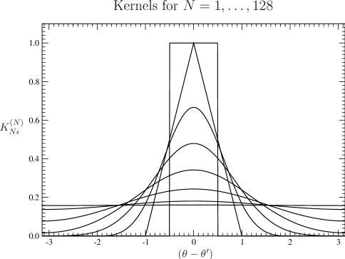
Figure 3: The kernels of several filters with increasing range $N\epsilon$, obtained via the use of their Fourier series, for $\epsilon=0.5$, for values of $N$ increasing exponentially, in the set $\{1,2,4,8,16,32,64,128\}$, plotted as functions of $\left(\theta-\theta^{\prime}\right)$ within the periodic interval $[-\pi,\pi]$.

A little numerical exploration is useful at this point to establish some simple mathematical facts about these infinite-order kernels. For completeness, let us go momentarily back to the straightforward multiple superposition of the first-order filter. If we take the $N\to\infty$ limit of the kernel of order $N$ with range $N\epsilon$, we might try to define a first infinite-order kernel with infinite range as

$$K_{\infty}^{(\infty)}\!\left(\theta-\theta^{\prime}\right)=\frac{1}{2\pi}+\frac{1}{\pi}\lim_{N\to\infty}\sum_{k=1}^{\infty}\left[\frac{\sin(k\epsilon)}{(k\epsilon)}\right]^{N}\cos\!\left[k\left(\theta-\theta^{\prime}\right)\right].$$

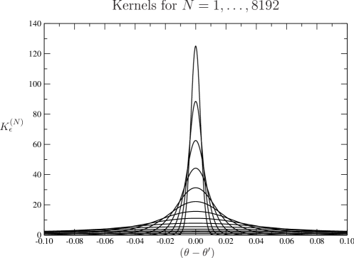
Figure 4: The kernels of several filters with constant range $\epsilon$, obtained via the use of their Fourier series, for $\epsilon=0.5$, for values of $N$ increasing exponentially, in the set $\{1,2,4,8,16,32,64,128,256,512,1024,2048,4096,8192\}$, plotted as functions of $\left(\theta-\theta^{\prime}\right)$ over a small sub-interval within the periodic interval $[-\pi,\pi]$.

Since this Fourier series converges very fast, and ever faster as $N$ increases, it is very easy to use it to plot the corresponding functions. Doing this one gets the sequence of functions shown in Figure 3. As expected, the range increases without bound and the kernel gets distributed more and more over the whole periodic interval, approaching a constant function with unit integral. This means that only the constant term of the Fourier expansion survives the limit, and that all the other Fourier coefficients converge to zero. There is nothing too surprising about this, since it is consistent with the fact that

$$\lim_{N\to\infty}\left[\frac{\sin(k\epsilon)}{(k\epsilon)}\right]^{N}=0,$$

so long as $\sin(k\epsilon)<(k\epsilon)$, which is true since $k>0$ and $\epsilon>0$. Once again a more rigorous analysis of this limit would require more careful consideration of the convergence of the series, since in principle one must be careful with the interchange of the $N\to\infty$ limit and the $k\to\infty$ limit of the series. However, here too it turns out that this rough discussion suffices for our purposes. It is quite clear that, if we could repeat the experiment on the whole real line instead of the periodic interval, the kernel would approach a normalized Gaussian function that in turn would approach zero everywhere, becoming ever wider and lower as $N\to\infty$.

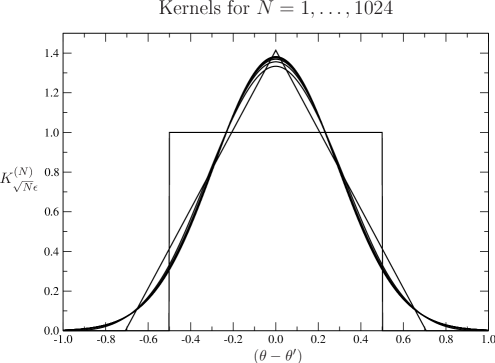
Figure 5: The kernels of several filters with Gaussian range $\sqrt{N}\epsilon$, obtained via the use of their Fourier series, for $\epsilon=0.5$, for values of $N$ increasing exponentially, in the set $\{1,2,4,8,16,32,64,128,256,512,1024\}$, plotted as functions of $\left(\theta-\theta^{\prime}\right)$ over a sub-interval within the periodic interval $[-\pi,\pi]$.

If we now consider once again the $N\to\infty$ limit of the kernel of order $N$ with constant range $\epsilon$, we might try to define an infinite-order kernel of finite range $\epsilon$ as

$$K_{\epsilon}^{(\infty)}\!\left(\theta-\theta^{\prime}\right)=\frac{1}{2\pi}+\frac{1}{\pi}\lim_{N\to\infty}\sum_{k=1}^{\infty}\left[\frac{\sin(k\epsilon/N)}{(k\epsilon/N)}\right]^{N}\cos\!\left[k\left(\theta-\theta^{\prime}\right)\right].$$

Our previous analysis indicated that this has the delta “function” as its limit. Plotting this kernel one gets the sequence of functions shown in Figure 4. As one can see, the kernel in fact diverges to positive infinity at zero. It also seems to go to zero everywhere else. Since it still has constant integral, and since it can be easily verified that its maximum at zero diverges to infinity as $\sqrt{N}$, we must conclude that it in fact approaches a Dirac delta “function”. More precisely, the sequence of kernels approaches a normalized Gaussian function that in turns approaches the delta “function”, becoming ever taller and narrower as $N\to\infty$, with constant area under the graph. What we have here is a singular limit, in a way going full circle, from the delta “function” at $N=0$ and back to it at $N\to\infty$. Therefore the $N\to\infty$ limit of this order-$N$ kernel is not a $C^{\infty}$ function, but a singular object instead, which is certainly an unexpected and surprising result.

This suggests that one may take an intermediate limit, which perhaps will converge to a non-singular localized function, by superposing $N$ filters with range $\sqrt{N}\epsilon$, thus obtaining a second infinite-order kernel with infinite range, given by

$$K_{\infty}^{(\infty)}\!\left(\theta-\theta^{\prime}\right)=\frac{1}{2\pi}+\frac{1}{\pi}\lim_{N\to\infty}\sum_{k=1}^{\infty}\left[\frac{\sin\!\left(k\epsilon/\sqrt{N}\right)}{\left(k\epsilon/\sqrt{N}\right)}\right]^{N}\cos\!\left[k\left(\theta-\theta^{\prime}\right)\right].$$

In fact, this exercise results in the sequence of functions seen in Figure 5, which approaches very fast a function very similar to a normalized Gaussian function with finite and non-zero width. Again it is quite clear that, if we could repeat this construction on the whole real line, then the limit would be a normalized Gaussian function, but in our case here it is a bit deformed by its containment within the periodic interval. When its width is small when compared to the length $2\pi$ of the periodic interval the Gaussian approaches zero very fast when we go significantly away from its point of maximum, so that we may consider this case to be paracompact, and even use this filter successfully in the practice of physics applications. However, the exact mathematical fact is that the range of this filter does tend to infinity when $N\to\infty$, and therefore to the whole extent of the periodic interval, if we execute all this operation within it.

It is possible to interpret qualitatively what happens in these three cases in terms of the expression for the corresponding superpositions of inner analytic functions. In the case of the straight multiple superposition of the first-order kernel we have for the representation of the order-$N$ filter on the complex plane

$$w_{N\epsilon}^{(N)}(z)=\left(\frac{-\mbox{\boldmath$\imath$}}{2\epsilon}\right)^{N}\sum_{n=0}^{N}\frac{(-1)^{n}N!}{n!(N-n)!}\,w^{-N\mbox{\Large$\cdot$}\!}\!\left(z\,{\rm e}^{\mbox{\boldmath$\imath$}[N-2n]\epsilon}\right),$$

where we may assume that the coefficients do not diverge with $N$, since the function tends to a constant everywhere on the unit circle in the $N\to\infty$ limit. In the case of the superposition of the first-order kernel with decreasing range $\epsilon/N$, resulting on a fixed range $\epsilon$ for the order-$N$ kernel, the representation of the order-$N$ filter in the complex plane is

$$w_{\epsilon}^{(N)}(z)=\left(\frac{-\mbox{\boldmath$\imath$}N}{2\epsilon}\right)^{N}\sum_{n=0}^{N}\frac{(-1)^{n}N!}{n!(N-n)!}\,w^{-N\mbox{\Large$\cdot$}\!}\!\left(z\,{\rm e}^{\mbox{\boldmath$\imath$}[1-2n/N]\epsilon}\right),$$

so that the extra factor of $N^{N}$ is clearly related to the divergence at a point on the unit circle, when we make $N\to\infty$. In the case of the superposition of the first-order kernel with decreasing range $\epsilon/\sqrt{N}$, resulting on a range $\sqrt{N}\epsilon$ for the order-$N$ kernel, the representation of the order-$N$ filter in the complex plane is

$$w_{\sqrt{N}\epsilon}^{(N)}(z)=\left(\frac{-\mbox{\boldmath$\imath$}\sqrt{N}}{2\epsilon}\right)^{N}\sum_{n=0}^{N}\frac{(-1)^{n}N!}{n!(N-n)!}\,w^{-N\mbox{\Large$\cdot$}\!}\!\left(z\,{\rm e}^{\mbox{\boldmath$\imath$}\left[\sqrt{N}-2n/\sqrt{N}\right]\epsilon}\right).$$

Note that in this case we gained a factor of $N^{N/2}$ rather than $N^{N}$, which the consequence that over the unit circle the kernel neither approaches a constant everywhere nor diverges to infinity somewhere. In this case the coefficients seem to have well-defined finite limits.

We must therefore conclude that, with this type of multiple superposition of the first-order filter, and the corresponding superposition of the singularities of the inner analytic functions in the complex plane, we are unable to define an infinite-order kernel that is both a finite and smooth real function, and that at the same time is localized within a compact support, thus generating an infinite-order filter with a finite range $\epsilon$. In order to understand why, it is useful to look at the singularities, on the unit circle of the complex plane, of the sequence of inner analytic functions generated by the repeated application of the first-order filter, starting with the inner analytic function corresponding to the zero-order kernel, which is a Dirac delta “function” and thus has a single first-order pole at some point on the unit circle, as shown in [1].

If we look at the diagram in Figure 2, we see that as the multiple application of the first-order filter goes on, more and more softened singularities are superposed at the points near the center of the diagram. Each singularity is progressively softer, but they are superposed in increasing numbers, thus generating a coefficient in the corresponding term in the superposition shown in Equation (6). For each finite $N$ these coefficients may be large, but they are finite, and therefore they do not disturb the softness of the corresponding singularities. However, if one of the coefficients diverges in the $N\to\infty$ limit, then the corresponding singularity is no longer soft in the limit. Let us recall that the definition of a soft singularity, as given in [2], is that the limit of the inner analytic function to that point be finite. Because of the diverging coefficients, in this type of superposition this may fail to be so in the $N\to\infty$ limit, even if the singularities are soft for each finite value of $N$.

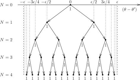
Figure 6: The scaled iteration of the first-order filter to produce an order-$N$ filter, showing the range $\epsilon_{N}$ tending to the limit $\epsilon$. The original singularity is at $\theta^{\prime}$. The numbers near the vertices of the triangles show that there is just one softened singularity at each such point.

We are therefore led to the idea of changing the method of iteration of the first-order filters in such a way that the softened singularities never get superposed. It is not too difficult to see that one may accomplish this by superposing filters with progressively smaller ranges, as illustrated by the diagram in Figure 6. Given a value of $\epsilon$, this diagram corresponds to a process in which we start by applying the first-order filter with range $\epsilon/2$, followed by the first-order filter of range $\epsilon/4$, then by the filter of range $\epsilon/8$, and so on, where the range of the $N^{\rm th}$ filter applied is given by $\epsilon/2^{N}$. Note that at the $N^{\rm th}$ iteration there are $2^{N}$ singularities homogeneously distributed within the interval $(-\epsilon,\epsilon)$. Since the ranges are scaled down exponentially, we call this a scaled filter, and the corresponding kernel a scaled kernel.

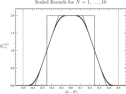
Figure 7: The kernels of several scaled filters with range $\epsilon_{N}\to\epsilon$, obtained via the use of their Fourier series, for $\epsilon=0.5$, for values of $N$ increasing linearly, in the set $\{1,2,3,4,5,6,7,8,9,10\}$, plotted as functions of $\left(\theta-\theta^{\prime}\right)$ over the support interval $[-\epsilon,\epsilon]$. The dashed lines mark the ends of the support interval.

At the $N^{\rm th}$ iteration there are $2^{N}$ singularities, each one softened by $N$ degrees, spaced from one another by $\epsilon/2^{N-1}$, and spaced from the ends of the $[-\epsilon,\epsilon]$ interval by $\epsilon/2^{N}$. They are, therefore, regularly distributed within the interval $(-\epsilon,\epsilon)$, centered at $2^{N}$ consecutive sub-intervals of length $\epsilon/2^{N-1}$. In the $N\to\infty$ limit the singularities will tend to become homogeneously distributed within the interval $(-\epsilon,\epsilon)$, and indeed will tend to a countable infinity of infinitely soft singularities distributed densely within that interval. Since at the $N^{\rm th}$ step there are $2^{N}$ such singularities, we see that their number grows exponentially fast. However, the singularities never get superposed. The corresponding superposition in terms of inner analytic functions in the complex plane is given by

$$\bar{w}_{\epsilon_{N}}^{(N)}(z) = \left(\frac{-2^{1}\mbox{\boldmath$\imath$}}{\epsilon}\right)\left(\frac{-2^{2}\mbox{\boldmath$\imath$}}{\epsilon}\right)\times\ldots\times\left(\frac{-2^{N-1}\mbox{\boldmath$\imath$}}{\epsilon}\right)\left(\frac{-2^{N}\mbox{\boldmath$\imath$}}{\epsilon}\right)\times$$

$$\hskip 70.0001pt\times\sum_{n=1}^{2^{N}}(-1)^{n-1}w^{-N\mbox{\Large$\cdot$}\!}\!\left(z\,{\rm e}^{\mbox{\boldmath$\imath$}\left[1-(2n-1)/2^{N}\right]\epsilon}\right)$$

$$= \left(\frac{-\mbox{\boldmath$\imath$}}{\epsilon}\right)^{N}2^{N(N+1)/2}\sum_{n=1}^{2^{N}}(-1)^{n-1}w^{-N\mbox{\Large$\cdot$}\!}\!\left(z\,{\rm e}^{\mbox{\boldmath$\imath$}\left[1-(2n-1)/2^{N}\right]\epsilon}\right).$$

Using the property of the first-order filter regarding its action on Fourier expansions [10, 11], it is not difficult to write the Fourier expansion of this new scaled kernel, at the $N^{\rm th}$ step of the construction process, which has a range $\epsilon_{N}$ such that $\epsilon/2\leq\epsilon_{N}<\epsilon$,

$$\bar{K}_{\epsilon_{N}}^{(N)}\!\left(\theta-\theta^{\prime}\right)=\frac{1}{2\pi}+\frac{1}{\pi}\sum_{k=1}^{\infty}\left[\frac{\sin\!\left(k\epsilon/2^{1}\right)}{\left(k\epsilon/2^{1}\right)}\right]\times\ldots\times\left[\frac{\sin\!\left(k\epsilon/2^{N}\right)}{\left(k\epsilon/2^{N}\right)}\right]\cos\!\left[k\left(\theta-\theta^{\prime}\right)\right],$$

where the coefficients include a product of $N$ different sinc factors. This product can be written as

$$\left[\frac{\sin\!\left(k\epsilon/2^{1}\right)}{\left(k\epsilon/2^{1}\right)}\right]\times\ldots\times\left[\frac{\sin\!\left(k\epsilon/2^{N}\right)}{\left(k\epsilon/2^{N}\right)}\right] = \frac{2^{1+\ldots+N}}{(k\epsilon)^{N}}\,\sin\!\left(\frac{k\epsilon}{2^{1}}\right)\times\ldots\times\sin\!\left(\frac{k\epsilon}{2^{N}}\right)$$

$$= \frac{2^{N(N+1)/2}}{(k\epsilon)^{N}}\prod_{n=1}^{N}\sin\!\left(\frac{k\epsilon}{2^{n}}\right).$$

It follows that we have for this order-$N$ scaled kernel

$$\bar{K}_{\epsilon_{N}}^{(N)}\!\left(\theta-\theta^{\prime}\right)=\frac{1}{2\pi}+\frac{1}{\pi}\sum_{k=1}^{\infty}\frac{2^{N(N+1)/2}}{(k\epsilon)^{N}}\left[\,\prod_{n=1}^{N}\sin\!\left(\frac{k\epsilon}{2^{n}}\right)\right]\cos\!\left[k\left(\theta-\theta^{\prime}\right)\right].$$ (7)

As expected, this kernel indeed has a well-defined limit when $N\to\infty$, with support in the finite interval $\left[\theta^{\prime}-\epsilon,\theta^{\prime}+\epsilon\right]$, as one can see in the graph of Figure 7. The sequence of kernels converges exponentially fast to a definite function, with a rather unusual shape.

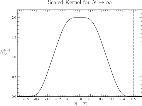
Figure 8: The best approximation of the kernel of the scaled filter with constant range $\epsilon$, in the $N\to\infty$ limit, obtained via the use of its Fourier series, for $\epsilon=0.5$, for a large value of $N$ ($100$), plotted as a function of $\left(\theta-\theta^{\prime}\right)$ over the support interval $[-\epsilon,\epsilon]$. The dashed lines mark the ends of the support interval.

It is possible to demonstrate explicitly the convergence of the sequence of scaled kernels $\bar{K}_{\epsilon_{N}}^{(N)}\!\left(\theta-\theta^{\prime}\right)$ to a well-defined regular function $\bar{K}_{\epsilon}^{(\infty)}\!\left(\theta-\theta^{\prime}\right)$ in the $N\to\infty$ limit. The proof is rather lengthy and is presented in full in Appendix B. It depends on the following facts about this limit, that we may establish here in order to give a general idea of the structure of the proof. First of all, due to one of the properties of the first-order filter [8] all kernels in the sequence have unit integral. Second, the range $\epsilon_{N}$ of the order-$N$ kernel is given by the combined ranges of all the kernels used to build it, and is therefore given by

$$\epsilon_{N}=\frac{\epsilon}{2}+\frac{\epsilon}{4}+\ldots+\frac{\epsilon}{2^{N-1}}+\frac{\epsilon}{2^{N}},$$

which is a geometric progression with ratio $1/2$. We have therefore

$$\epsilon_{N} = \epsilon\,\frac{{\displaystyle\frac{\displaystyle 1}{\displaystyle 2}}-{\displaystyle\frac{\displaystyle 1}{\displaystyle 2^{N+1}}}}{1-{\displaystyle\frac{\displaystyle 1}{\displaystyle 2}}}$$

$$= \epsilon\left(1-\frac{1}{2^{N}}\right).$$

It follows therefore that in the $N\to\infty$ limit $\epsilon_{N}$ tends to $\epsilon$,

$$\lim_{N\to\infty}\epsilon_{N}=\epsilon.$$

Therefore all the kernels in the sequence remain identically zero everywhere outside the interval $(-\epsilon,\epsilon)$, so that we may conclude that the limiting function has support within that interval. Next we observe that, since the filtered function is defined as an average of the original function, it can never assume values which are larger than the maximum of the function it is applied on, or smaller than its minimum. Therefore, since the first kernel we start with, with range $\epsilon/2$, is limited within the interval $[0,1/\epsilon]$, so are all the subsequent kernels of the construction sequence.

As a consequence all these considerations, the non-zero parts of the graphs of all the kernels in the construction sequence are contained within the rectangle defined by the support interval $[-\epsilon,\epsilon]$ and the range of values $[0,1/\epsilon]$, which has area $2$. The area of the graph of every kernel in the construction sequence is $1$, so that it occupies one half of the area of the rectangle. Since every scaled kernel in the construction sequence is a continuous and differentiable function, it becomes clear that the $N\to\infty$ limit of the sequence of kernels must also be a regular function within this rectangle. It follows from the discussion in Appendix B that the limit of the sequence exists and is a regular, continuous and differentiable function, resulting in the infinite-order scaled kernel with range $\epsilon$

$$\bar{K}_{\epsilon}^{(\infty)}\!\left(\theta-\theta^{\prime}\right)=\lim_{N\to\infty}\bar{K}_{\epsilon_{N}}^{(N)}\!\left(\theta-\theta^{\prime}\right).$$

This infinite-order scaled kernel has the deceptively simple look shown in Figure 8. Despite appearances it contains no completely straight segments within its support interval. Once it is shown that it is a $C^{\infty}$ function, it follows that its derivatives of all orders are zero at the two extremes of the support interval, where they must match the correspondingly zero derivatives of the two external segments, on either side of the support interval, where the kernel is identically zero.

A technical note about the graphs representing the $N\to\infty$ limit of various quantities is in order at this point. They were obtained numerically from the corresponding Fourier series, using the scaled filter of order $N=100$. This means that the last first-order filter used in the multiple superposition has a range of $\epsilon/2^{100}$. This is less than $\epsilon/10^{30}$ and is therefore many orders of magnitude below any graphical resolution one might hope for, in any medium. Certainly the errors related to the summation of the Fourier series, which were set at $10^{-12}$, are the dominant ones, but still extremely small. We may conclude that these graphs are faithful representations of the corresponding quantities for all conceivable graphical purposes. The programs used in creating all the graphs shown in this paper are freely available online [12].

It is quite simple to see that this kernel is a $C^{\infty}$ function. Its Fourier series, given as the $N\to\infty$ limit of the Fourier expansion in Equation (7), is certainly absolutely and uniformly convergent, and any finite-order term-wise derivative of it results in another series with the same properties. Since the convergence of the resulting series is the additional condition, besides uniform convergence, that suffices to guarantee that one can differentiate the series term-wise in order to obtain the derivative of the function, we may conclude that derivatives of all finite orders exist and are given by continuous and differentiable functions. This proof of infinite differentiability of the $\bar{K}_{\epsilon}^{(\infty)}\!\left(\theta-\theta^{\prime}\right)$ kernel now ensures that the kernel and all its multiple derivatives are in fact zero at the points $\left(\theta-\theta^{\prime}\right)=\pm\epsilon$.

An independent discussion of the existence of the derivatives of all finite orders can be found in Section B.7 of Appendix B. There one can see also that the derivatives of all orders are zero at the central point of maximum, as well as at the two extremes of the support interval. We also show in Section B.8 of Appendix B that the infinite-order scaled kernel is not analytic as a function on the periodic interval, in the real sense of the term. We do this by showing that there is a countable infinity of points, distributed densely in the support interval, where only a finite number of derivatives is different from zero. We also discuss briefly there the question of whether or not the infinite-order scaled kernel can be extended analytically to the complex plane. We discuss this in terms of the fact that it is the limit of an inner analytic function when one takes the limit to the border of the unit disk.

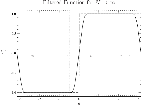
Figure 9: The filtered square wave and the parameters related to the action of the infinite-order scaled filter, obtained via the use of its Fourier series, for $\epsilon=0.5$, for a large value of $N$ ($100$), plotted as a function of $\theta$ over the periodic interval $[-\pi,\pi]$. The original function is shown with the dashed line and the filtered function with the solid line. The dotted lines mark the intervals where the function was changed by the filter.

Given that the infinite-order scaled kernel is a $C^{\infty}$ function, one may then define an infinite-order filter based on this infinite-order scaled kernel. However, in this case it is not so simple to determine the form of the coefficients directly in the $N\to\infty$ limit. In fact, the question of whether or not it is possible to write the coefficients directly in the $N\to\infty$ limit, in some simple form, is an open one. Note that, as was mentioned before, one must be careful with the interchange of the $N\to\infty$ limit and the $k\to\infty$ limit of the series. In any case, it follows that given any merely integrable function $f(\theta)$, the filtered function

$$f_{\epsilon}^{(\infty)}(\theta)=\int_{-\infty}^{\infty}d\theta^{\prime}\,\bar{K}_{\epsilon}^{(\infty)}\!\left(\theta-\theta^{\prime}\right)f\!\left(\theta^{\prime}\right),$$

is necessarily a $C^{\infty}$ function, in the real sense of the term. It is easy to see this, since the differentiations with respect to $\theta$ at the right-hand side will act only on the infinite-order scaled kernel, which is a $C^{\infty}$ function. Therefore all the finite-order derivatives of $f_{\epsilon}^{(\infty)}(\theta)$ exist, since they may be written as

$$\frac{d^{n}}{d\theta^{n}}f_{\epsilon}^{(\infty)}(\theta)=\int_{-\infty}^{\infty}d\theta^{\prime}\left[\frac{d^{n}}{d\theta^{n}}\bar{K}_{\epsilon}^{(\infty)}\!\left(\theta-\theta^{\prime}\right)\right]f\!\left(\theta^{\prime}\right),$$

where the $n^{\rm th}$ derivative of the infinite-order scaled kernel is a limited, continuous and differentiable function with compact support, being therefore an integrable function. In addition to this, the changes made in $f(\theta)$ in order to produce $f_{\epsilon}^{(\infty)}(\theta)$ have a finite range $\epsilon$ that can be made as small as one wishes.

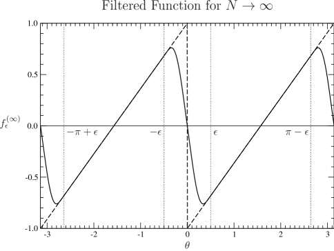
Figure 10: The filtered sawtooth wave wave and the parameters related to the action of the infinite-order scaled filter, obtained via the use of its Fourier series, for $\epsilon=0.5$, for a large value of $N$ ($100$), plotted as a function of $\theta$ over the periodic interval $[-\pi,\pi]$. The original function is shown with the dashed line and the filtered function with the solid line. The dotted lines mark the intervals where the function was changed by the filter.

Let us now consider the action of such a filter on inner analytic functions. There is no difficulty in determining what happens to the singularities of the inner analytic functions on the unit circle, as a consequence of the application of this infinite-order scaled filter. It is quite clear that a single singularity of the inner analytic function at $\theta$ would be smeared into a denumerable infinity of softened singularities within the interval $[\theta-\epsilon,\theta+\epsilon]$ on the unit circle. This set of singularities would occupy the interval densely, and they would be infinitely soft, since they are the result of an infinite sequence of logarithmic integrations. Since each logarithmic integration renders the real function on the unit circle differentiable to one more order, in the limit one gets over that circle an infinitely differentiable real function of $\theta$. So the resulting complex function of $z$ must be an inner analytic function which has only infinitely soft singularities on the unit circle and that is a $C^{\infty}$ function of $\theta$ when restricted to that circle. The same is true for the kernel itself, if we start with a single first-order pole at $\theta$, which is the case for the order-zero kernel. Note that in either case this real function is $C^{\infty}$ right on top of a densely-distributed set of singularities of the corresponding inner analytic function, which is somewhat unexpected, even if they are infinitely soft singularities.

As a simple example, let us consider the unit-amplitude square wave, which is a discontinuous periodic function, as one can see in Figure 9, that shows the filtered function superposed with the original one. The filtered function was obtained from its Fourier series, which due to the properties of the first-order filter is easily obtained, being given by

$$f_{\epsilon_{N}}(\theta)=\frac{4}{\pi}\sum_{j=0}^{\infty}\frac{2^{N(N+1)/2}}{k^{N+1}\epsilon^{N}}\left[\,\prod_{n=1}^{N}\sin\!\left(\frac{k\epsilon}{2^{n}}\right)\right]\sin\!\left(k\theta\right),$$

where $k=2j+1$, for a large value of $N$. The graph of the original function has two straight horizontal segments and two points of discontinuity at $\theta=0$ and at $\theta=\pm\pi$. It follows that the corresponding inner analytic function has two borderline hard singularities at these two points. Let us consider all the instances of the first-order linear low-pass filter used for the construction of the infinite-order scaled kernel, for all construction steps $N$ and any value of $\epsilon<\pi$. Since the linear low-pass filters are all the identity on the segments that are linear functions, up to a distance of $\epsilon$ to one of the singularities, the function would never be changed at all outside the two intervals $[-\epsilon,\epsilon]$ and $[\pi-\epsilon,-\pi+\epsilon]$, when one applies to it any of the order-$N$ scaled filters. After the end of the process of application of the infinite-order scaled filter these two intervals would contain segments of $C^{\infty}$ functions of $\theta$, and in fact the whole resulting function would be a $C^{\infty}$ function of $\theta$, over the whole unit circle.

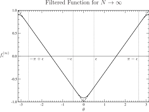
Figure 11: The filtered triangular wave and the parameters related to the action of the infinite-order scaled filter, obtained via the use of its Fourier series, for $\epsilon=0.5$, for a large value of $N$ ($100$), plotted as a function of $\theta$ over the periodic interval $[-\pi,\pi]$. The original function is shown with the dashed line and the filtered function with the solid line. The dotted lines mark the intervals where the function was changed by the filter.

Another similar example can be seen in Figure 10, which shows the case of the unit-amplitude sawtooth wave, which also has the same two points of discontinuity and therefore corresponds to an inner analytic function with two similar borderline hard singularities at these points. The filtered function was obtained from its Fourier series,

$$f_{\epsilon_{N}}(\theta)=-\,\frac{4}{\pi}\sum_{j=1}^{\infty}\frac{2^{N(N+1)/2}}{k^{N+1}\epsilon^{N}}\left[\,\prod_{n=1}^{N}\sin\!\left(\frac{k\epsilon}{2^{n}}\right)\right]\sin\!\left(k\theta\right),$$

where $k=2j$, for a large value of $N$. In Figure 11 one can see the case of the triangular wave, which is a continuous function with two points of non-differentiability at $\theta=0$ and at $\theta=\pm\pi$, and therefore corresponds to an inner analytic function with two borderline soft singularities at these points. The filtered function was obtained from its Fourier series,

$$f_{\epsilon_{N}}(\theta)=-\,\frac{8}{\pi^{2}}\sum_{j=0}^{\infty}\frac{2^{N(N+1)/2}}{k^{N+2}\epsilon^{N}}\left[\,\prod_{n=1}^{N}\sin\!\left(\frac{k\epsilon}{2^{n}}\right)\right]\cos\!\left(k\theta\right),$$

where $k=2j+1$, for a large value of $N$. In all cases we chose a rather large value for $\epsilon$ as compared to its maximum value $\pi$, namely $0.5$, in order to render the action of the scaled infinite-order filter clearly visible. What we seem to have here is a factory of $C^{\infty}$ functions of $\theta$ on the unit circle. Starting with virtually any integrable function, we may consider the application of the infinite-order scaled filter in order to produce a $C^{\infty}$ function on the unit circle, making changes only with a range $\epsilon$ that can be as small as we wish.

Once we have the infinite-order scaled filter defined within the periodic interval, it is simple to extend it to the whole real line. Considering that the infinite-order scaled kernel and all its derivatives are zero at the two ends of its support interval, we may just take that support interval and insert it into the real line. If we make the new infinite-order scaled kernel identically zero outside the support interval, in all the rest of the real line, we still have a $C^{\infty}$ function. This is so because at the two points of concatenation the two lateral limits of the kernel are equal, being both zero, as are the two lateral limits of its first derivative, and the same for all the higher-order derivatives. Therefore, we may also define an infinite-order scaled filter acting on the whole real line, that maps any integrable real function to corresponding $C^{\infty}$ functions.

4 Conclusions

Linear low-pass filters of arbitrary orders can be easily and elegantly defined on the complex plane, within the unit disk, acting on inner analytic functions. Within the open unit disk the filter simply maps inner analytic functions onto other inner analytic functions. Through the correspondence of these functions with FC pairs of DP Fourier series, these filters reproduce the linear low-pass filters that were defined in a previous paper, acting on the corresponding DP real functions defined on the unit circle. Several of the properties of these filters are then clearly in view, given the known properties of that correspondence.

The effect of the first-order low-pass filter, as seen in the complex plane, is characterized as a process of singularity splitting, in which each singularity of an inner analytic function on the unit circle is exchanged for two softer singularities over that same circle. This has the effect of improving the convergence characteristics of the DP Fourier series, and also of rendering the corresponding DP real functions smoother after the filtering process. Higher-order filters correspond to the iteration of this process on the unit circle, producing ever larger collections of ever softer singularities on that circle.

A discussion of the problems encountered when one tries to define an infinite-order low-pass filter acting on real functions, in the most immediate way, led to the detailed construction of such an infinite-order filter, within a compact support. The representation of the filters in the complex plane was instrumental for the success of this construction. The infinite-order filter is defined in terms of an infinite-order scaled kernel, with compact support given by a real parameter $\epsilon$, which can be as small as one wishes.

The infinite-order scaled kernel is defined as the limit of a sequence of order-$N$ scaled kernels, and proof of the convergence of the sequence was presented. It was also shown that the infinite-order scaled kernel is a $C^{\infty}$ real function, but not an analytic real function. The infinite-order scaled kernel can be given in a fairly explicit way as a limit of a Fourier series, which converges extremely fast. Once the infinite-order filter is defined in the periodic interval, it is a simple matter to define a corresponding infinite-order filter that acts on the whole real line.

This infinite-order scaled filter, acting on any merely integrable real function on the unit circle, has as its result a real function that is $C^{\infty}$ on the unit circle, while making on the original function only changers with the finite range $\epsilon$. The same is true for real function defined on the whole real line. Therefore, one obtains as a result of this construction a tool that can produce from any integrable real function corresponding $C^{\infty}$ functions, making changes only within a range $\epsilon$ that can be as small as desired.

This allows us to use these filters in physics applications, if we use values of $\epsilon$ sufficiently small in order not to change the description of the physics within the physically relevant scales of any given problem. By reducing the value of $\epsilon$ these $C^{\infty}$ functions can be made as close as one wishes to the corresponding original functions, according to a criterion that has a clear physical meaning, as explained in a previous paper.

In addition to this, the construction of the filter is equivalent to proof that there are many real functions that are $C^{\infty}$ but that are not analytic, and that are typically not extensible analytically to the complex plane. The filter can be used to produce examples of such functions in copious quantities. It is quite easy to obtain accurate values for the filtered functions by numerical means, and thus to represent the action of the filter in practical applications.

5 Acknowledgements

The author would like to thank his friend and colleague Prof. Carlos Eugênio Imbassay Carneiro, to whom he is deeply indebted for all his interest and help, as well as his careful reading of the manuscript and helpful criticism regarding this work.

Appendix A Appendix: Technical Proofs

A.1 Direct Derivation of the Coefficients $a_{\epsilon,k}$

Let us determine the effect of the first-order linear low-pass filter, defined on the complex plane, on the coefficients $a_{k}$. We start with the Taylor coefficients of $w(z)$, which can be written in terms of its real an imaginary parts,

$$w(z)=f_{\rm c}(\rho,\theta)+\mbox{\boldmath$\imath$}f_{\rm s}(\rho,\theta),$$

in terms of which the Taylor coefficients are given by

$$a_{k} = \frac{\rho^{-k}}{\pi}\int_{-\pi}^{\pi}d\theta\,f_{\rm c}(\rho,\theta)\cos(k\theta)$$

$$= \frac{\rho^{-k}}{\pi}\int_{-\pi}^{\pi}d\theta\,f_{\rm s}(\rho,\theta)\sin(k\theta).$$

The Taylor coefficients of $w_{\epsilon}(z)$ are similarly given by

$$a_{\epsilon,k} = \frac{\rho^{-k}}{\pi}\int_{-\pi}^{\pi}d\theta\,f_{\epsilon,{\rm c}}(\rho,\theta)\cos(k\theta)$$

$$= \frac{\rho^{-k}}{\pi}\int_{-\pi}^{\pi}d\theta\,f_{\epsilon,{\rm s}}(\rho,\theta)\sin(k\theta).$$

Let us work out only the first case, involving the cosine, since the work for the second one in essentially identical and leads to the same result. Using the definition of $f_{\epsilon,{\rm c}}(\rho,\theta)$ in terms of $f_{\rm c}(\rho,\theta)$ we have

$$a_{\epsilon,k} = \frac{\rho^{-k}}{\pi}\int_{-\pi}^{\pi}d\theta\,\cos(k\theta)\,\frac{1}{2\epsilon}\int_{\theta-\epsilon}^{\theta+\epsilon}d\theta^{\prime}\,f_{\rm c}\!\left(\rho,\theta^{\prime}\right)$$

$$= -\,\frac{\rho^{-k}}{2\epsilon\pi}\int_{-\pi}^{\pi}d\theta\,\frac{\sin(k\theta)}{k}\,\frac{d}{d\theta}\int_{\theta-\epsilon}^{\theta+\epsilon}d\theta^{\prime}\,f_{\rm c}\!\left(\rho,\theta^{\prime}\right)$$

$$= -\,\frac{\rho^{-k}}{2\epsilon\pi k}\int_{-\pi}^{\pi}d\theta\,\sin(k\theta)\;f_{\rm c}\!\left(\rho,\theta^{\prime}\right)\left.\rule{0.0pt}{12.91663pt}\right[_{\,\theta-\epsilon}^{\,\theta+\epsilon}$$

$$= -\,\frac{\rho^{-k}}{2\epsilon\pi k}\int_{-\pi}^{\pi}d\theta\,\sin(k\theta)f_{\rm c}(\rho,\theta+\epsilon)+\frac{\rho^{-k}}{2\epsilon\pi k}\int_{-\pi}^{\pi}d\theta\,\sin(k\theta)f_{\rm c}(\rho,\theta-\epsilon),$$

where we integrated by parts and where there is no integrated term due to the periodicity of the integrand in $\theta$. We now change variables in each integral, using $\theta^{\prime}=\theta\pm\epsilon$, in order to obtain

$$a_{\epsilon,k} = -\,\frac{\rho^{-k}}{2\epsilon\pi k}\int_{-\pi}^{\pi}d\theta^{\prime}\,\sin\!\left(k\theta^{\prime}-k\epsilon\right)f_{\rm c}\!\left(\rho,\theta^{\prime}\right)+\frac{\rho^{-k}}{2\epsilon\pi k}\int_{-\pi}^{\pi}d\theta^{\prime}\,\sin\!\left(k\theta^{\prime}+k\epsilon\right)f_{\rm c}\!\left(\rho,\theta^{\prime}\right)$$

$$= \frac{\rho^{-k}}{2\epsilon\pi k}\int_{-\pi}^{\pi}d\theta^{\prime}\,f_{\rm c}\!\left(\rho,\theta^{\prime}\right)\left[\sin\!\left(k\theta^{\prime}+k\epsilon\right)-\sin\!\left(k\theta^{\prime}-k\epsilon\right)\right],$$

where the integration limits did not change in the transformations of variables due to the periodicity of the integrand. Changing $\theta^{\prime}$ back to $\theta$ we are left with

$$a_{\epsilon,k} = \frac{\rho^{-k}}{2\epsilon\pi k}\int_{-\pi}^{\pi}d\theta\,f_{\rm c}\!\left(\rho,\theta\right)\left[\sin(k\theta)\cos(k\epsilon)+\sin(k\epsilon)\cos(k\theta)\right.+$$

$$\hskip 90.00014pt-\left.\sin(k\theta)\cos(k\epsilon)+\sin(k\epsilon)\cos(k\theta)\right]$$

$$= \left[\frac{\sin(k\epsilon)}{(k\epsilon)}\right]\frac{\rho^{-k}}{\pi}\int_{-\pi}^{\pi}d\theta\,f_{\rm c}\!\left(\rho,\theta\right)\cos(k\theta).$$

Since we recover in this way the expression of the coefficients of $f_{\rm c}(\rho,\theta)$, we get

$$a_{\epsilon,k}=\left[\frac{\sin(k\epsilon)}{(k\epsilon)}\right]a_{k},$$

which is the same result obtained in the text through the application of the filter, as an operator, to the expansion of $w(z)$. This more direct derivation bypasses any preoccupations with the convergence of the series during that process, due to the term-wise application of the integral operator.

A.2 Alternate Proof of the Inner Analyticity of $w_{\epsilon}(z)$

Here we establish that $w_{\epsilon}(z)$ is analytic by showing that its real and imaginary parts satisfy the Cauchy-Riemann conditions. Consider an inner analytic function $w(z)$ and the corresponding filtered function within the open unit disk, with the real angular parameter $0<\epsilon\leq\pi$

$$w_{\epsilon}(z)=\frac{1}{2\epsilon}\int_{\theta-\epsilon}^{\theta+\epsilon}d\theta^{\prime}\,w\!\left(z^{\prime}\right).$$

Since $w(z)$ is analytic, we have $w(z)=f_{\rm c}(\rho,\theta)+\mbox{\boldmath$\imath$}f_{\rm s}(\rho,\theta)$ where $f_{\rm c}(\rho,\theta)$ and $f_{\rm s}(\rho,\theta)$ satisfy the Cauchy-Riemann conditions in polar coordinates,

$$\frac{\partial f_{\rm c}}{\partial\rho}(\rho,\theta) = \frac{1}{\rho}\,\frac{\partial f_{\rm s}}{\partial\theta}(\rho,\theta),$$

$$\frac{1}{\rho}\,\frac{\partial f_{\rm c}}{\partial\theta}(\rho,\theta) = -\,\frac{\partial f_{\rm s}}{\partial\rho}(\rho,\theta).$$

It follows that the filtered function can be written as

$$w_{\epsilon}(z) = f_{\epsilon,{\rm c}}(\rho,\theta)+\mbox{\boldmath$\imath$}f_{\epsilon,{\rm s}}(\rho,\theta)$$

$$= \frac{1}{2\epsilon}\int_{\theta-\epsilon}^{\theta+\epsilon}d\theta^{\prime}\,f_{\rm c}\!\left(\rho,\theta^{\prime}\right)+\mbox{\boldmath$\imath$}\,\frac{1}{2\epsilon}\int_{\theta-\epsilon}^{\theta+\epsilon}d\theta^{\prime}\,f_{\rm s}\!\left(\rho,\theta^{\prime}\right),$$

so that we have

$$f_{\epsilon,{\rm c}}(\rho,\theta) = \frac{1}{2\epsilon}\int_{\theta-\epsilon}^{\theta+\epsilon}d\theta^{\prime}\,f_{\rm c}\!\left(\rho,\theta^{\prime}\right),$$

$$f_{\epsilon,{\rm s}}(\rho,\theta) = \frac{1}{2\epsilon}\int_{\theta-\epsilon}^{\theta+\epsilon}d\theta^{\prime}\,f_{\rm s}\!\left(\rho,\theta^{\prime}\right).$$

Since $f_{\rm c}(\rho,\theta)$ and $f_{\rm s}(\rho,\theta)$ are continuous and differentiable, it is clear that so are $f_{\epsilon,{\rm c}}(\rho,\theta)$ and $f_{\epsilon,{\rm s}}(\rho,\theta)$. If we calculate their partial derivatives with respect to $\rho$ we get

$$\frac{\partial f_{\epsilon,{\rm c}}}{\partial\rho}(\rho,\theta) = \frac{1}{2\epsilon}\int_{\theta-\epsilon}^{\theta+\epsilon}d\theta^{\prime}\,\frac{\partial f_{\rm c}}{\partial\rho}\!\left(\rho,\theta^{\prime}\right),$$

$$\frac{\partial f_{\epsilon,{\rm s}}}{\partial\rho}(\rho,\theta) = \frac{1}{2\epsilon}\int_{\theta-\epsilon}^{\theta+\epsilon}d\theta^{\prime}\,\frac{\partial f_{\rm s}}{\partial\rho}\!\left(\rho,\theta^{\prime}\right).$$

Using the Cauchy-Riemann relations for $w(z)$ we may write these as

$$\frac{\partial f_{\epsilon,{\rm c}}}{\partial\rho}(\rho,\theta) = \frac{1}{2\epsilon}\int_{\theta-\epsilon}^{\theta+\epsilon}d\theta^{\prime}\,\frac{1}{\rho}\,\frac{\partial f_{\rm s}}{\partial\theta}\!\left(\rho,\theta^{\prime}\right)$$

$$= \frac{1}{\rho}\,\frac{1}{2\epsilon}\,f_{\rm s}\!\left(\rho,\theta^{\prime}\right)\left.\rule{0.0pt}{12.91663pt}\right[_{\,\theta-\epsilon}^{\,\theta+\epsilon},$$

$$= \frac{1}{\rho}\,\frac{f_{\rm s}(\rho,\theta+\epsilon)-f_{\rm s}(\rho,\theta-\epsilon)}{2\epsilon},$$

$$\frac{\partial f_{\epsilon,{\rm s}}}{\partial\rho}(\rho,\theta) = -\,\frac{1}{2\epsilon}\int_{\theta-\epsilon}^{\theta+\epsilon}d\theta^{\prime}\,\frac{1}{\rho}\,\frac{\partial f_{\rm c}}{\partial\theta}\!\left(\rho,\theta^{\prime}\right)$$

$$= -\,\frac{1}{\rho}\,\frac{1}{2\epsilon}\,f_{\rm c}\!\left(\rho,\theta^{\prime}\right)\left.\rule{0.0pt}{12.91663pt}\right[_{\,\theta-\epsilon}^{\,\theta+\epsilon}$$

$$= -\,\frac{1}{\rho}\,\frac{f_{\rm c}(\rho,\theta+\epsilon)-f_{\rm c}(\rho,\theta-\epsilon)}{2\epsilon}.$$

If we now calculate the partial derivatives of $f_{\epsilon,{\rm c}}(\rho,\theta)$ and $f_{\epsilon,{\rm s}}(\rho,\theta)$ with respect to $\theta$ we get

$$\frac{1}{\rho}\,\frac{\partial f_{\epsilon,{\rm c}}}{\partial\theta}(\rho,\theta) = \frac{1}{\rho}\,\frac{1}{2\epsilon}\,\frac{\partial}{\partial\theta}\int_{\theta-\epsilon}^{\theta+\epsilon}d\theta^{\prime}\,f_{\rm c}\!\left(\rho,\theta^{\prime}\right)$$

$$= \frac{1}{\rho}\,\frac{f_{\rm c}(\rho,\theta+\epsilon)-f_{\rm c}(\rho,\theta-\epsilon)}{2\epsilon},$$

$$\frac{1}{\rho}\,\frac{\partial f_{\epsilon,{\rm s}}}{\partial\theta}(\rho,\theta) = \frac{1}{\rho}\,\frac{1}{2\epsilon}\,\frac{\partial}{\partial\theta}\int_{\theta-\epsilon}^{\theta+\epsilon}d\theta^{\prime}\,f_{\rm s}\!\left(\rho,\theta^{\prime}\right)$$

$$= \frac{1}{\rho}\,\frac{f_{\rm s}(\rho,\theta+\epsilon)-f_{\rm s}(\rho,\theta-\epsilon)}{2\epsilon}.$$

Comparing this pair of equations with the previous one we get

$$\frac{\partial f_{\epsilon,{\rm c}}}{\partial\rho}(\rho,\theta) = \frac{1}{\rho}\,\frac{\partial f_{\epsilon,{\rm s}}}{\partial\theta}(\rho,\theta),$$

$$\frac{1}{\rho}\,\frac{\partial f_{\epsilon,{\rm c}}}{\partial\theta}(\rho,\theta) = -\,\frac{\partial f_{\epsilon,{\rm s}}}{\partial\rho}(\rho,\theta),$$

which establish the analyticity of $w_{\epsilon}(z)$, in the same domain as that of $w(z)$. Let us now examine the other properties defining an inner analytic function. For one thing we have $w(0)=0$, which means that

$$\lim_{\rho\to 0}f_{\rm c}(\rho,\theta) = 0,$$

$$\lim_{\rho\to 0}f_{\rm s}(\rho,\theta) = 0.$$

If we calculate the corresponding limits for $w_{\epsilon}(z)$ we get

$$\lim_{\rho\to 0}f_{\epsilon,{\rm c}}(\rho,\theta) = \lim_{\rho\to 0}\frac{1}{2\epsilon}\int_{\theta-\epsilon}^{\theta+\epsilon}d\theta^{\prime}\,f_{\rm c}\!\left(\rho,\theta^{\prime}\right)$$

$$= \frac{1}{2\epsilon}\int_{\theta-\epsilon}^{\theta+\epsilon}d\theta^{\prime}\,\lim_{\rho\to 0}f_{\rm c}\!\left(\rho,\theta^{\prime}\right)$$

$$= 0,$$

$$\lim_{\rho\to 0}f_{\epsilon,{\rm s}}(\rho,\theta) = \lim_{\rho\to 0}\frac{1}{2\epsilon}\int_{\theta-\epsilon}^{\theta+\epsilon}d\theta^{\prime}\,f_{\rm s}\!\left(\rho,\theta^{\prime}\right)$$

$$= \frac{1}{2\epsilon}\int_{\theta-\epsilon}^{\theta+\epsilon}d\theta^{\prime}\,\lim_{\rho\to 0}f_{\rm s}\!\left(\rho,\theta^{\prime}\right)$$

$$= 0.$$

We have therefore that $w_{\epsilon}(0)=0$. Finally, $w(z)$ reduces to a real function over the interval $(-1,1)$ of the real axis, which means that its imaginary part is zero there, and therefore that $f_{\rm s}(\rho,0)=0$ and $f_{\rm s}(\rho,\pm\pi)=0$. If we write $f_{\epsilon,{\rm s}}(\rho,\theta)$ for the same values of $\theta$ we get

$$f_{\epsilon,{\rm s}}(\rho,0) = \frac{1}{2\epsilon}\int_{-\epsilon}^{\epsilon}d\theta^{\prime}\,f_{\rm s}\!\left(\rho,\theta^{\prime}\right),$$

$$f_{\epsilon,{\rm s}}(\rho,\pm\pi) = \frac{1}{2\epsilon}\int_{\pm\pi-\epsilon}^{\pm\pi+\epsilon}d\theta^{\prime}\,f_{\rm s}\!\left(\rho,\theta^{\prime}\right)$$

$$= \frac{1}{2\epsilon}\int_{-\pi-\epsilon}^{\pi+\epsilon}d\theta^{\prime}\,f_{\rm s}\!\left(\rho,\theta^{\prime}\right).$$

However, since $w(z)$ is an inner analytic function we have that $f_{\rm s}(\rho,\theta)$ is an odd function of $\theta$. In both cases above this implies that the integral is zero, and hence we conclude that $w_{\epsilon}(z)$ is an inner analytic function as well.

A.3 Proof of Analyticity of $w_{\varepsilon}(z)$ in the Cartesian Case

As a curiosity, it is interesting to point out that a first-order linear low-pass filter can be defined over a straight segment on the complex plane. In this way a filter in the Cartesian coordinates of the complex plane can be defined. Consider an analytic function $w(z)$ anywhere on the complex plane. Consider also a segment of length $2\varepsilon$ and a fixed direction given by a constant angle $\alpha$ with the real axis. Given an arbitrary position $z$ on the complex plane we define then two other points by

$$z_{\oplus} = z+\varepsilon\,{\rm e}^{\mbox{\boldmath$\imath$}\alpha},$$

$$z_{\ominus} = z-\varepsilon\,{\rm e}^{\mbox{\boldmath$\imath$}\alpha}.$$

This defines a segment of length $2\varepsilon$ going from $z_{\ominus}$ to $z_{\oplus}$. Given any point $z$ such that this segment is contained within the analyticity domain of $w(z)$, we may now define a filtered function $w_{\varepsilon}(z)$ by

$$w_{\varepsilon}(z) = \frac{1}{2\varepsilon}\int_{z_{\ominus}}^{z_{\oplus}}dz^{\prime}\,w\!\left(z^{\prime}\right)$$

$$= \frac{\,{\rm e}^{\mbox{\boldmath$\imath$}\alpha}}{2\varepsilon}\int_{-\varepsilon}^{\varepsilon}d\lambda\,w\!\left(z+\lambda\,{\rm e}^{\mbox{\boldmath$\imath$}\alpha}\right),$$

where $\lambda$ is a real parameter describing the segment, such that $-\varepsilon\leq\lambda\leq\varepsilon$ and

$$z^{\prime} = z+\lambda\,{\rm e}^{\mbox{\boldmath$\imath$}\alpha}\;\;\;\Rightarrow$$

$$dz^{\prime} = \,{\rm e}^{\mbox{\boldmath$\imath$}\alpha}d\lambda.$$

Since $w(z)=u(x,y)+\mbox{\boldmath$\imath$}v(x,y)$ is analytic, $u(x,y)$ and $v(x,y)$ are continuous, differentiable and satisfy the Cauchy-Riemann conditions in Cartesian coordinates. We may write for $w_{\varepsilon}(z)$

$$w_{\varepsilon}(z) = u_{\varepsilon}(x,y)+\mbox{\boldmath$\imath$}v_{\varepsilon}(x,y)$$

$$= \frac{\,{\rm e}^{\mbox{\boldmath$\imath$}\alpha}}{2\varepsilon}\int_{-\varepsilon}^{\varepsilon}d\lambda\,\left\{\rule{0.0pt}{10.76385pt}u[x+\lambda\cos(\alpha),y+\lambda\sin(\alpha)]\right.+$$

$$\hskip 50.00008pt+\left.\mbox{\boldmath$\imath$}v[x+\lambda\cos(\alpha),y+\lambda\sin(\alpha)]\rule{0.0pt}{10.76385pt}\right\}\;\;\;\Rightarrow$$

$$u_{\varepsilon}(x,y) = \frac{\,{\rm e}^{\mbox{\boldmath$\imath$}\alpha}}{2\varepsilon}\int_{-\varepsilon}^{\varepsilon}d\lambda\,u[x+\lambda\cos(\alpha),y+\lambda\sin(\alpha)],$$

$$v_{\varepsilon}(x,y) = \frac{\,{\rm e}^{\mbox{\boldmath$\imath$}\alpha}}{2\varepsilon}\int_{-\varepsilon}^{\varepsilon}d\lambda\,v[x+\lambda\cos(\alpha),y+\lambda\sin(\alpha)].$$

It is now clear that $u_{\varepsilon}(x,y)$ and $v_{\varepsilon}(x,y)$ are also continuous and differentiable. If we now take the partial derivatives of these functions with respect to $x$ we get

$$\frac{\partial u_{\varepsilon}}{\partial x}(x,y) = \frac{\,{\rm e}^{\mbox{\boldmath$\imath$}\alpha}}{2\varepsilon}\int_{-\varepsilon}^{\varepsilon}d\lambda\,\frac{\partial u}{\partial x}[x+\lambda\cos(\alpha),y+\lambda\sin(\alpha)],$$

$$\frac{\partial v_{\varepsilon}}{\partial x}(x,y) = \frac{\,{\rm e}^{\mbox{\boldmath$\imath$}\alpha}}{2\varepsilon}\int_{-\varepsilon}^{\varepsilon}d\lambda\,\frac{\partial v}{\partial x}[x+\lambda\cos(\alpha),y+\lambda\sin(\alpha)].$$

Using the Cauchy-Riemann conditions for $u(x,y)$ and $v(x,y)$ we get

$$\frac{\partial u_{\varepsilon}}{\partial x}(x,y) = \frac{\,{\rm e}^{\mbox{\boldmath$\imath$}\alpha}}{2\varepsilon}\int_{-\varepsilon}^{\varepsilon}d\lambda\,\frac{\partial v}{\partial y}[x+\lambda\cos(\alpha),y+\lambda\sin(\alpha)],$$

$$\frac{\partial v_{\varepsilon}}{\partial x}(x,y) = -\,\frac{\,{\rm e}^{\mbox{\boldmath$\imath$}\alpha}}{2\varepsilon}\int_{-\varepsilon}^{\varepsilon}d\lambda\,\frac{\partial u}{\partial y}[x+\lambda\cos(\alpha),y+\lambda\sin(\alpha)].$$

Taking now the partial derivatives of $u_{\varepsilon}(x,y)$ and $v_{\varepsilon}(x,y)$ with respect to $y$ we get

$$\frac{\partial u_{\varepsilon}}{\partial y}(x,y) = \frac{\,{\rm e}^{\mbox{\boldmath$\imath$}\alpha}}{2\varepsilon}\int_{-\varepsilon}^{\varepsilon}d\lambda\,\frac{\partial u}{\partial y}[x+\lambda\cos(\alpha),y+\lambda\sin(\alpha)],$$

$$\frac{\partial v_{\varepsilon}}{\partial y}(x,y) = \frac{\,{\rm e}^{\mbox{\boldmath$\imath$}\alpha}}{2\varepsilon}\int_{-\varepsilon}^{\varepsilon}d\lambda\,\frac{\partial v}{\partial y}[x+\lambda\cos(\alpha),y+\lambda\sin(\alpha)].$$

Comparing this pair of equation with the previous ones we finally get

$$\frac{\partial u_{\varepsilon}}{\partial x}(x,y) = \frac{\partial v_{\varepsilon}}{\partial y}(x,y),$$

$$\frac{\partial u_{\varepsilon}}{\partial y}(x,y) = -\,\frac{\partial v_{\varepsilon}}{\partial x}(x,y).$$

This establishes that $u_{\varepsilon}(x,y)$ and $v_{\varepsilon}(x,y)$ satisfy the Cauchy-Riemann conditions, and therefore that $w_{\varepsilon}(z)$ is analytic. Once $w_{\varepsilon}(z)$ is defined by the filter at all points of the domain of analyticity of $w(z)$ where the segment fits, and now that it has been proven analytic there, one can extend the definition of $w_{\varepsilon}(z)$ to the whole domain of analyticity of $w(z)$ by analytic continuation.

Appendix B Proof of Convergence to the Infinite-Order Kernel

In this appendix we will offer proof of the convergence of the sequence of order-$N$ scaled kernels to the infinite-order scaled kernel, in the $N\to\infty$ limit. The point is to show that the infinite sequence of real functions $\bar{K}_{\epsilon_{N}}^{(N)}(\theta)$, with $\epsilon<\pi$, converges in the $N\to\infty$ limit to a definite regular real function with finite support within $[-\epsilon,\epsilon]$, which we denote as $\bar{K}_{\epsilon}^{(\infty)}(\theta)$. In addition to this, we will establish that the infinite-order scaled kernel $\bar{K}_{\epsilon}^{(\infty)}(\theta)$ is a $C^{\infty}$ function, and that it is not an analytic function in the real sense of the term.

In order to do this we must first establish a few more properties of the first-order filter, in addition to those demonstrated in [3]. We will also have to examine more closely some aspects of the process of construction of the infinite-order scaled kernel.

B.1 Invariance of the Sign of the First Derivative

According to one of the properties established before for the first-order filter [5], if $f(\theta)$ is continuous in the domain where the filter is applied, then $f_{\epsilon}(\theta)$ is differentiable, and its derivative is given by

$$\frac{df_{\epsilon}(\theta)}{d\theta}=\frac{f\!\left(\theta+\epsilon\right)-f\!\left(\theta-\epsilon\right)}{2\epsilon}.$$ (8)

This is valid so long as the support interval of the filter fits completely inside the region where $f(\theta)$ is continuous. This immediately implies that, in a region where $f(\theta)$ increases monotonically we have

$$f\!\left(\theta+\epsilon\right) \geq f\!\left(\theta-\epsilon\right)\;\;\;\Rightarrow$$

$$\frac{df_{\epsilon}(\theta)}{d\theta} \geq 0.$$

We may therefore conclude that $f_{\epsilon}(\theta)$ also increases monotonically within the sub-region where the support interval of the filter fits inside the region in which $f(\theta)$ is continuous. In the same way, in a region where $f(\theta)$ decreases monotonically we have

$$f\!\left(\theta+\epsilon\right) \leq f\!\left(\theta-\epsilon\right)\;\;\;\Rightarrow$$

$$\frac{df_{\epsilon}(\theta)}{d\theta} \leq 0.$$

We may therefore conclude that $f_{\epsilon}(\theta)$ also decreases monotonically within that same sub-region. In other words, the monotonic character of the variation of a function is invariant by the action of the filter. In particular, at points where $f(\theta)$ is differentiable the sign of its derivative is invariant by the action of the filter.

B.2 Invariance of the Sign of the Second Derivative

If we assume that $f(\theta)$ is differentiable in the domain where the filter is applied, then $f_{\epsilon}(\theta)$ can be differentiated twice, and we may obtain its second derivative by simply differentiating once Equation (8), which results in

$$\frac{d^{2}f_{\epsilon}(\theta)}{d\theta^{2}}=\frac{1}{2\epsilon}\left[\frac{df}{d\theta}\!\left(\theta+\epsilon\right)-\frac{df}{d\theta}\!\left(\theta-\epsilon\right)\right].$$

This is valid so long as the support interval of the filter fits completely inside the region where $f(\theta)$ is differentiable. This immediately implies that, in a region where the derivative of $f(\theta)$ increases monotonically we have

$$\frac{df}{d\theta}\!\left(\theta+\epsilon\right) \geq \frac{df}{d\theta}\!\left(\theta-\epsilon\right)\;\;\;\Rightarrow$$

$$\frac{d^{2}f_{\epsilon}(\theta)}{d\theta^{2}} \geq 0.$$

We may therefore conclude that the derivative of $f_{\epsilon}(\theta)$ also increases monotonically within the sub-region where the support interval of the filter fits inside the region in which $f(\theta)$ is differentiable. In the same way, in a region where the derivative of $f(\theta)$ decreases monotonically we have

$$\frac{df}{d\theta}\!\left(\theta+\epsilon\right) \leq \frac{df}{d\theta}\!\left(\theta-\epsilon\right)\;\;\;\Rightarrow$$

$$\frac{d^{2}f_{\epsilon}(\theta)}{d\theta^{2}} \leq 0.$$

We may therefore conclude that the derivative of $f_{\epsilon}(\theta)$ also decreases monotonically within that same sub-region. In other words, the monotonic character of the variation of the derivative of a function is invariant by the action of the filter. In particular, at points where $f(\theta)$ is twice differentiable the sign of its second derivative is invariant by the action of the filter.

This implies that in regions where the second derivative of $f(\theta)$ has constant sign, and therefore the concavity of its graph is turned in a definite direction, up or down, the action of the filter keeps that concavity turned in the same direction. In other words, away from inflection points, in regions where the graph of $f(\theta)$ has a definite concavity turned in a definite direction, $f_{\epsilon}(\theta)$ has the same concavity, turned in the same direction.

B.3 Action of the Filter in Regions of Definite Concavity

Consider the action of the first-order filter in a region where the graph of $f(\theta)$ has definite concavity, turned in a definite direction, and within which the support interval of the filter fits. As shown in [4], if $f(\theta)$ happens to be a linear function within the support of the filter around a given point, then the filter is the identity and therefore $f_{\epsilon}(\theta)=f(\theta)$ at that point. On the other hand, if $f(\theta)$ is not a linear function and its concavity is turned down, them some values of the function within the support of the filter must be smaller that in the case of the linear function. Since the filtered function $f_{\epsilon}(\theta)$ is defined as an average of the values of $f(\theta)$, it follows that, if the concavity of the graph of $f(\theta)$ is turned down, then

$$f_{\epsilon}(\theta)<f(\theta).$$

In the same way, we may conclude that if the concavity of the graph of $f(\theta)$ is turned up, then

$$f_{\epsilon}(\theta)>f(\theta).$$

In other words, in regions where the function $f(\theta)$ has its concavity turned in a definite direction, and within which the support interval of the filter fits, the action of the filter always changes the value of the function in the direction to which its concavity is turned.

B.4 Bounds of the Scaled Kernels

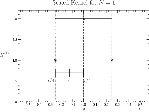
Figure 12: The scaled kernel for $\epsilon=0.5$ and $N=1$, plotted as a function of $\theta$ over the support interval $[-\epsilon,\epsilon]$. The five invariant points are marked by stars, and the support interval of the next filter in the construction sequence is shown. The dashed lines mark the center and the two ends of the support interval, and hence three of the five invariant points. The dotted lines mark the sectors where the function is defined in a piece-wise fashion.

Let us observe that since the filtered function $f_{\epsilon}(\theta)$ is defined as an average of the function $f(\theta)$, it can never assume values which are larger than the maximum of the function it is applied on, or smaller than its minimum, without regard to the value of the range $\epsilon$. Therefore, since the first kernel we start with in the process of construction of the infinite-order scaled kernel, that is the kernel $\bar{K}_{\epsilon_{1}}^{(1)}(\theta)$, with $N=1$ and range $\epsilon/2$, is bound within the interval $[0,1/\epsilon]$ for all values of $\theta$, so is the next one, the kernel $\bar{K}_{\epsilon_{2}}^{(2)}(\theta)$. We may now apply the same argument to this second kernel, and conclude that the third one in the sequence is also bound in the same way, and so on. It follows that, for all values of $N$, we have

$$0\leq\bar{K}_{\epsilon_{N}}^{(N)}(\theta)\leq\frac{1}{\epsilon},$$

for all values of $\theta$ within the periodic interval $[-\pi,\pi]$, and in particular for all values of $\theta$ within the support interval $[-\epsilon,\epsilon]$. It also follows that, if the $N\to\infty$ limit of the sequence of kernel functions exists, then it is also bound in the same way.

B.5 Invariant Points of the Scaled Kernels

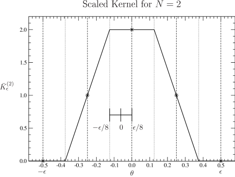
Figure 13: The scaled kernel for $\epsilon=0.5$ and $N=2$, plotted as a function of $\theta$ over the support interval $[-\epsilon,\epsilon]$. The five invariant points are marked by stars, and the support interval of the next filter in the construction sequence is shown. The dashed lines mark the four intervals defined by the five invariant points. The dotted lines mark the sectors where the function is defined in a piece-wise fashion.

Let us now show that there are five points of the graphs of the order-$N$ scaled kernels that remain invariant throughout the construction of the infinite-order scaled kernel. These are the following: the point of maximum at $\theta=0$, where the value of the kernel function is $1/\epsilon$; the two points of minimum at $\theta=\pm\epsilon$, where the value is zero; and the two inflection points at $\theta=\pm\epsilon/2$, where the value is $1/(2\epsilon)$. These five points are marked with stars on the graphs in Figures 12, 13 and 14, which display the first three kernels in the construction sequence. Note that in the case of the discontinuous $N=1$ kernel in Figure 12 we choose the values at the points of discontinuity according to the criterion of the average of the lateral limits, which defines these two future points of inflection in a way that is compatible with this invariance.

Note now that in Figure 12 the points of maximum and minimum are within sectors where the kernel function is linear, in intervals of size $\epsilon$ (or more, in the case of the points of minimum) around these points. The support of the next filter to be applied, in the sequence leading to the construction of the infinite-order scaled kernel, is also shown in the graph. Since this support has length $\epsilon/2$, it fits into the intervals where the kernel function is linear, in which case it acts as the identity, according to one of the properties of the first-order filter [4]. Therefore, after the application of this next filter intervals of length $\epsilon/2$ will remain around these three points, where the next kernel function so generated is still linear.

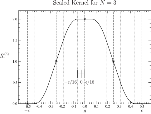
Figure 14: The scaled kernel for $\epsilon=0.5$ and $N=3$, plotted as a function of $\theta$ over the support interval $[-\epsilon,\epsilon]$. The five invariant points are marked by stars, and the support interval of the next filter in the construction sequence is shown. The dashed lines mark the four intervals defined by the five invariant points. The dotted lines mark the sectors where the function is defined in a piece-wise fashion.

The result of this operation, which is the $N=2$ scaled kernel, is shown in Figure 13. Note that in this case all the five points listed before have around them intervals of length $\epsilon/2$ where the kernel function is linear. Once more the support of the next filter to be applied, in the sequence leading to the construction of the infinite-order scaled kernel, is shown in the graph. Since this support has length $\epsilon/4$, it fits into the intervals where the kernel function is linear, in which case it acts as the identity, so that after its application intervals of length $\epsilon/4$ will remain around all these five points, where the next kernel function generated is still linear. In particular, this will keep the points invariant, since they are within sectors where the kernel functions are linear and hence where the first-order filter acts as the identity.

The result of this last operation, which is the $N=3$ scaled kernel, is shown in Figure 14. Once again all five points are within sectors of length $\epsilon/4$ where the kernel function is linear. Since the support of the next filter to be applied has now length $\epsilon/8$, once more it will keep these points invariant. It is now quite clear that both the length of the linear sectors and the length of the support of the next filter will be scaled down exponentially during the process of construction of the infinite-order kernel, with the support being always half the length of the intervals, and therefore fitting within them. This establishes that the five points we listed here are in fact invariant throughout the construction of the infinite-order scaled kernel. In particular, it follows that these are the values of the infinite-order scaled kernel function at these five points, and that the sequence of order-$N$ scaled kernel functions in fact converges to the infinite-order scaled kernel function at these five points.

B.6 Convergence of the Scaled Kernels

We are now ready to show that the sequence of order-$N$ scaled kernels converges to the infinite-order scaled kernel, within the whole support interval. Of course the convergence is guaranteed outside the support interval, since all the scaled kernels in the construction sequence are identically zero there. Starting from the $N=3$ scaled kernel shown in Figure 14, which is an everywhere continuous and differentiable function, we consider the action on it of the next first-order filter. Observe that within each one of the four intervals of length $\epsilon/2$ defined by the five invariant points this kernel is monotonic, and also that its first derivative is monotonic as well. The situation is as follows: in the first interval $[-\epsilon,-\epsilon/2]$ both the kernel function and its derivative are monotonically increasing; in the second interval $[-\epsilon/2,0]$ the kernel function is monotonically increasing, but its derivative is monotonically decreasing; in the third interval $[0,\epsilon/2]$, both the kernel function and its derivative are monotonically decreasing; in the fourth interval $[\epsilon/2,\epsilon]$, the kernel function is monotonically decreasing, but its derivative is monotonically increasing.

This means that this kernel function has a definite concavity in each of the four intervals. Let us now consider the action of the next instance of the first-order filter, at each point within the final support interval $[-\epsilon,\epsilon]$. We can say that either one of the five invariant points is contained within the support of the filter, or none is. If one of them is contained in the support, then we have already established that the support of the filter is contained within an interval where the kernel function is linear, and therefore the filter acts as the identity. In this case the kernel function is not changed at all. Otherwise, the support is contained within one of the four intervals where the kernel function has a definite concavity. In this case the kernel function will be changed, but its monotonic character, and that of its derivative, will be preserved. In other words the next kernel will have the same monotonicity and concavity properties on the same four intervals. Since this argument can then be iterated, we conclude that all subsequent kernel functions in the construction sequence have these same monotonicity and concavity properties, on the same four intervals.

Let us now consider the action of the first-order filter at any subsequent stage of the construction process. Once again, we have that either one of the five invariant points is contained within the support of the current filter, or none is. If one of the points is contained in the support, then the support of the filter is contained within an interval where the current kernel function is linear, and therefore the filter acts as the identity, so that the value of the kernel function is not changed. If none of the five points is contained within the support, then that support is contained within one of the four intervals where the current kernel has the same monotonicity and concavity properties of all the others in the sequence, starting with $N=3$. This means that at all stages of the construction process the points of the graph of the current kernel will always be changed in the same direction within these four intervals, being therefore always increased in the intervals $[-\epsilon,-\epsilon/2]$ and $[\epsilon/2,\epsilon]$, and always decreased in the intervals $[-\epsilon/2,0]$ and $[0,\epsilon/2]$.

What we may conclude from this is that, given any value of $\theta$ within $[-\epsilon,\epsilon]$, either it is one of the invariant points, at which all order-$N$ kernel functions have the same values, and therefore where the sequence of kernel functions converges, or it is a point strictly within one of the four intervals where the kernel functions have definite monotonicity and concavity properties. In this case the sequence of values of the order-$N$ kernel functions at that point form a monotonic real sequence. Since this is a monotonic sequence of real numbers that is bound from below by zero and from above by $1/\epsilon$, it follows that the sequence converges. Since we may therefore state that the point-wise convergence holds for all points within the final support interval $[-\epsilon,\epsilon]$, and recalling that outside this interval all order-$N$ kernels are identically zero, we conclude the the sequence of order-$N$ scales kernels converges, in the $N\to\infty$ limit, to the infinite-order scaled kernel, a definite limited real function $\bar{K}_{\epsilon}^{(\infty)}(\theta)$ with compact support.

B.7 Differentiability of the Infinite-Order Scaled Kernel

The infinite-order scaled kernel with finite range $\epsilon$ has an interesting property of its own, namely that there is a certain similarity between the kernel and its derivatives. Every finite-order derivative of the infinite-order scaled kernel function is made out of a certain number of rescaled copies of the kernel itself, concatenated together. This is a consequence of the fact that there is a certain relation between the first derivative of the order-$N$ scaled kernel and the order-$(N-1)$ scaled kernel. After this relation is established it can be iterated, resulting in similar relations for the higher-order derivatives. This property allows one to establish the existence of the $N\to\infty$ limits of all the finite-order derivatives, and thus to prove that the infinite-order scaled kernel is differentiable to all orders.

One can derive the relation between the first derivative of the order-$N$ scaled kernel and the order-$(N-1)$ scaled kernel as follows. If we start with the Fourier expansion of the order-$N$ scaled kernel, written in the form

$$\bar{K}_{\epsilon_{N}}^{(N)}(\theta)=\frac{1}{2\pi}+\frac{1}{\pi}\sum_{k=1}^{\infty}\left[\,\prod_{n=1}^{N}\frac{\sin\!\left(k\epsilon/2^{n}\right)}{\left(k\epsilon/2^{n}\right)}\right]\cos(k\theta),$$

we may differentiate once term-by-term and thus obtain

$$\frac{d}{d\theta}\bar{K}_{\epsilon_{N}}^{(N)}(\theta) = \frac{1}{\pi}\sum_{k=1}^{\infty}\left[\frac{\sin\!\left(k\epsilon/2^{1}\right)}{\left(k\epsilon/2^{1}\right)}\right]\left[\,\prod_{n=2}^{N}\frac{\sin\!\left(k\epsilon/2^{n}\right)}{\left(k\epsilon/2^{n}\right)}\right](-k)\sin(k\theta)$$

$$= \frac{1}{\pi\epsilon}\sum_{k=1}^{\infty}\left[\,\prod_{n=2}^{N}\frac{\sin\!\left(k\epsilon/2^{n}\right)}{\left(k\epsilon/2^{n}\right)}\right]\left[-2\sin\!\left(k\epsilon/2\right)\sin(k\theta)\right],$$

noting that for sufficiently large $N$ all the series involved are absolutely and uniformly convergent. By means of simple trigonometric identities the product of two sines within brackets can now be written as

$$-2\sin\!\left(k\epsilon/2\right)\sin(k\theta)=\cos\!\left[k\left(\theta+\epsilon/2\right)\right]-\cos\!\left[k\left(\theta-\epsilon/2\right)\right],$$

so that we have for the derivative of the kernel

$$\frac{d}{d\theta}\bar{K}_{\epsilon_{N}}^{(N)}(\theta) = \frac{1}{\pi\epsilon}\sum_{k=1}^{\infty}\left[\,\prod_{n=2}^{N}\frac{\sin\!\left(k\epsilon/2^{n}\right)}{\left(k\epsilon/2^{n}\right)}\right]\cos\!\left[k\left(\theta+\epsilon/2\right)\right]+$$

$$-\,\frac{1}{\pi\epsilon}\sum_{k=1}^{\infty}\left[\,\prod_{n=2}^{N}\frac{\sin\!\left(k\epsilon/2^{n}\right)}{\left(k\epsilon/2^{n}\right)}\right]\cos\!\left[k\left(\theta-\epsilon/2\right)\right].$$

Figure 15: The infinite-order scaled kernel (solid line) and its first derivative (dashed line), obtained via the use of their Fourier series, for $\epsilon=0.5$, for a large value of $N$ ($100$), plotted as functions of $\theta$ over the support interval $[-\epsilon,\epsilon]$. The derivative was rescaled down to have the same amplitude as the kernel. The dotted lines mark the points where the first derivative is zero.

If we now define $\epsilon^{\prime}=\epsilon/2$, we may write

$$\frac{d}{d\theta}\bar{K}_{\epsilon_{N}}^{(N)}(\theta) = \frac{2}{\pi\epsilon^{\prime}}\sum_{k=1}^{\infty}\left[\,\prod_{n=2}^{N}\frac{\sin\!\left(k\epsilon^{\prime}/2^{n-1}\right)}{\left(k\epsilon^{\prime}/2^{n-1}\right)}\right]\cos\!\left[k\left(\theta+\epsilon^{\prime}\right)\right]+$$

$$-\,\frac{2}{\pi\epsilon^{\prime}}\sum_{k=1}^{\infty}\left[\,\prod_{n=2}^{N}\frac{\sin\!\left(k\epsilon^{\prime}/2^{n-1}\right)}{\left(k\epsilon^{\prime}/2^{n-1}\right)}\right]\cos\!\left[k\left(\theta-\epsilon^{\prime}\right)\right]$$

$$= \frac{1}{2\pi}+\frac{2}{\pi\epsilon^{\prime}}\sum_{k=1}^{\infty}\left[\,\prod_{n^{\prime}=1}^{N-1}\frac{\sin\!\left(k\epsilon^{\prime}/2^{n^{\prime}}\right)}{\left(k\epsilon^{\prime}/2^{n^{\prime}}\right)}\right]\cos\!\left[k\left(\theta+\epsilon^{\prime}\right)\right]+$$

$$-\,\frac{1}{2\pi}-\frac{2}{\pi\epsilon^{\prime}}\sum_{k=1}^{\infty}\left[\,\prod_{n^{\prime}=1}^{N-1}\frac{\sin\!\left(k\epsilon^{\prime}/2^{n^{\prime}}\right)}{\left(k\epsilon^{\prime}/2^{n^{\prime}}\right)}\right]\cos\!\left[k\left(\theta-\epsilon^{\prime}\right)\right],$$

where we made $n^{\prime}=n-1$, which implies $n=n^{\prime}+1$. We see therefore that in this way we recover in the right-hand side the expression of the scaled kernel of order $N-1$ with range $\epsilon/2$, so that we have, writing $\epsilon^{\prime}$ back in terms of $\epsilon$,

$$\frac{d}{d\theta}\bar{K}_{\epsilon_{N}}^{(N)}(\theta)=\frac{1}{\epsilon}\left[\bar{K}_{\epsilon_{(N-1)}/2}^{(N-1)}\!\left(\theta+\epsilon/2\right)-\bar{K}_{\epsilon_{(N-1)}/2}^{(N-1)}\!\left(\theta-\epsilon/2\right)\right].$$

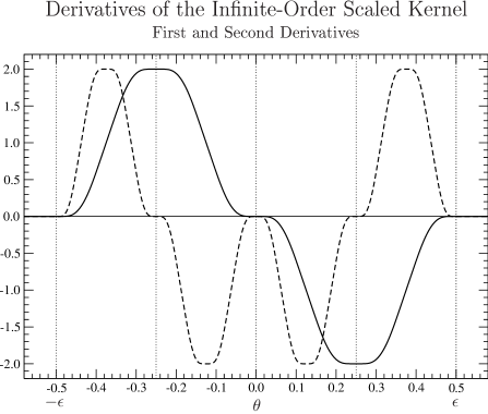
Figure 16: The first (solid line) and second (dashed line) derivatives of the infinite-order scaled kernel, obtained via the use of their Fourier series, for $\epsilon=0.5$, for a large value of $N$ ($100$), plotted as functions of $\theta$ over the support interval $[-\epsilon,\epsilon]$. Both derivatives were rescaled down to have the same amplitude as the kernel. The dotted lines mark the points where the second derivative is zero.

Since we already know that the $N\to\infty$ limit of the right-hand side exists, this establishes that the $N\to\infty$ limit of the left-hand exists as well. Taking the $N\to\infty$ limit we end up with the infinite-order scaled kernel on both sides, so that we have the relation

$$\frac{d}{d\theta}\bar{K}_{\epsilon}^{\infty}(\theta)=\frac{1}{\epsilon}\left[\bar{K}_{\epsilon/2}^{\infty}\!\left(\theta+\epsilon/2\right)-\bar{K}_{\epsilon/2}^{\infty}\!\left(\theta-\epsilon/2\right)\right].$$

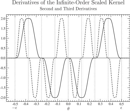
Figure 17: The second (solid line) and third (dashed line) derivatives of the infinite-order scaled kernel, obtained via the use of their Fourier series, for $\epsilon=0.5$, for a large value of $N$ ($100$), plotted as functions of $\theta$ over the support interval $[-\epsilon,\epsilon]$. Both derivatives were rescaled down to have the same amplitude as the kernel. The dotted lines mark the points where the third derivative is zero.

It follows therefore, as expected, that the infinite-order scaled kernel function is differentiable. Note that, since the kernels on the right-hand side have range $\epsilon/2$, and their points of application are distant from each other by exactly $\epsilon$, each one is just outside the support of the other. Therefore, the derivative is given by the concatenation of two graphs just like the kernel itself, but with the support scaled down from $\epsilon$ to $\epsilon/2$, with the amplitude scaled up by the factor $2/\epsilon$, and with the sign of one of them inverted. This is shown in Figure 15, containing a superposition of the kernel and its rescaled first derivative.

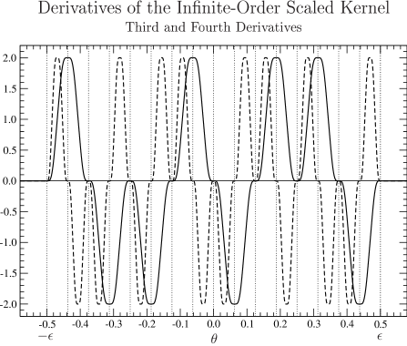
Figure 18: The third (solid line) and fourth (dashed line) derivatives of the infinite-order scaled kernel, obtained via the use of their Fourier series, for $\epsilon=0.5$, for a large value of $N$ ($100$), plotted as functions of $\theta$ over the support interval $[-\epsilon,\epsilon]$. Both derivatives were rescaled down to have the same amplitude as the kernel. The dotted lines mark the points where the fourth derivative is zero.

One may now take one more derivative of the expression for the derivative of the order-$N$ scaled kernel, thus obtaining an expression for the corresponding second derivative. After that one may use again the relation for the first derivative, thus iterating that relation, in order to obtain

$$\frac{d^{2}}{d\theta^{2}}\bar{K}_{\epsilon_{N}}^{(N)}(\theta) = \frac{1}{\epsilon}\left[\frac{d}{d\theta}\bar{K}_{\epsilon_{(N-1)}/2}^{(N-1)}\!\left(\theta+\epsilon/2\right)-\frac{d}{d\theta}\bar{K}_{\epsilon_{(N-1)}/2}^{(N-1)}\!\left(\theta-\epsilon/2\right)\right]$$

$$= \frac{1}{\epsilon}\left\{\frac{2}{\epsilon}\left[\bar{K}_{\epsilon_{(N-2)}/4}^{(N-2)}\!\left(\theta+3\epsilon/4\right)-\bar{K}_{\epsilon_{(N-2)}/4}^{(N-2)}\!\left(\theta+\epsilon/4\right)\right]\right.+$$

$$\hskip 20.00003pt-\left.\frac{2}{\epsilon}\left[\bar{K}_{\epsilon_{(N-2)}/4}^{(N-2)}\!\left(\theta-\epsilon/4\right)-\bar{K}_{\epsilon_{(N-2)}/4}^{(N-2)}\!\left(\theta-3\epsilon/4\right)\right]\right\}$$

$$= \frac{2}{\epsilon^{2}}\left[\bar{K}_{\epsilon_{(N-2)}/4}^{(N-2)}\!\left(\theta+3\epsilon/4\right)-\bar{K}_{\epsilon_{(N-2)}/4}^{(N-2)}\!\left(\theta+\epsilon/4\right)\right.+$$

$$\hskip 20.00003pt-\left.\bar{K}_{\epsilon_{(N-2)}/4}^{(N-2)}\!\left(\theta-\epsilon/4\right)+\bar{K}_{\epsilon_{(N-2)}/4}^{(N-2)}\!\left(\theta-3\epsilon/4\right)\right].$$

Once more the known existence of the $N\to\infty$ limit of the right-hand side establishes the existence of the $N\to\infty$ limit of the left-hand side, and therefore that the infinite-order scaled kernel is twice differentiable. Taking the limit on both sides we get

$$\frac{d^{2}}{d\theta^{2}}\bar{K}_{\epsilon}^{\infty}(\theta) = \frac{2}{\epsilon^{2}}\left[\bar{K}_{\epsilon/4}^{\infty}(\theta+3\epsilon/4)-\bar{K}_{\epsilon/4}^{\infty}(\theta+\epsilon/4)\right.+$$

$$\hskip 20.00003pt\left.-\bar{K}_{\epsilon/4}^{\infty}(\theta-\epsilon/4)+\bar{K}_{\epsilon/4}^{\infty}(\theta-3\epsilon/4)\right].$$

We now have four copies of the graph of the kernel, with range scaled down to $\epsilon/4$ and amplitude scaled up by $2/\epsilon^{2}$, each one outside the supports of the others, distributed in a regular way within the interval of length $2\epsilon$ around $\theta$. This is shown in Figure 16, containing a superposition of the rescaled first and second derivatives of the kernel. As one can see in the subsequent Figures 17 and 18, the same type of relationship is also true for all the higher-order derivatives. This is so because we can iterate this relation indefinitely, so that any finite-order derivative of $\bar{K}_{\epsilon}^{\infty}(\theta)$ can be written as a finite linear combination of $\bar{K}_{\epsilon}^{\infty}(\theta)$ itself, with a rescaled $\epsilon$ and a rescaled amplitude. Observe that this constitutes independent proof that the infinite-order scaled kernel is a $C^{\infty}$ function.

B.8 Non-Analyticity of the Infinite-Order Scaled Kernel

From the construction described in the previous section for the order-$n$ derivatives of the infinite-order scaled kernel, which can all be written in terms of the kernel itself, and from the fact that the infinite-order scaled kernel is zero at the two ends of its support interval, it follows at once that all the order-$n$ derivatives of the kernel are also zero at these two points. Therefore the kernel and all its order-$n$ derivatives, for all $n\geq 0$, are zero at the two ends $\theta=\pm\epsilon$ of the support interval, as in fact we already knew, since this is also a consequence of the fact that the kernel is a $C^{\infty}$ function over its whole domain.

In a similar way, we may also determine other points within the support interval where almost all the order-$n$ derivatives of the kernel are zero. For example, at the central point, although the kernel itself is not zero, we see that its first derivative is, and in fact iterating the construction one can see that all the higher-order derivatives are zero there. Therefore all the order-$n$ derivatives of the kernel, for all $n\geq 1$, are zero at the central point $\theta=0$ of the support interval. An examination of the situation at the two inflection points $\theta=\pm\epsilon/2$ reveals that at those two points all the order-$n$ derivatives of the kernel, for all $n\geq 2$, are zero.

Order	Number of points	Null Derivatives
0	$2$	$m\geq 0$
1	$3$	$m\geq 1$
2	$5$	$m\geq 2$
3	$9$	$m\geq 3$
4	$17$	$m\geq 4$
⋮	⋮	⋮
n	$2^{n}+1$	$m\geq n$
⋮	⋮	⋮

Table 1: Points where almost all derivatives of the infinite-order scaled kernel are zero. The integer $n$ is the order of the first null derivative, and $m$ gives the orders of all derivatives which are zero at the corresponding set of points.

The iteration of this process of analysis can be continued indefinitely, with the result that there are sets of increasing numbers of points regularly spaced in the support interval where all derivatives above a certain order are zero. This can be systematized as shown in Table 1. We see therefore that there is a set of $2^{n}+1$ points regularly spaced within the support interval where all derivatives with order $n$ or larger are zero. In the $n\to\infty$ limit this set of points tends to be densely distributed within the support interval. Outside the support interval the derivatives of all orders are zero at all points, of course, since the kernel is identically zero there.

In we assemble the Taylor series of the kernel function around one of the points where all the derivatives of order $n$ and larger are zero, we obtain a convergent power series, which is in fact a polynomial of order $n-1$. Since the kernel function is obviously not such a polynomial, it is therefore not represented by its convergent Taylor series around this reference point, at any points other than the reference point itself. Since in order to be analytic the kernel function would have to be so represented within an open set around the reference point, it follows that it is not analytic at any of these points. Since this set of points tends to become densely distributed within the support interval, we may conclude that the kernel function is not analytic at all points of the support interval.

One can try to extend this argument to show in a somewhat heuristic way that the kernel function cannot be represented by a convergent power series around any point of the support interval, whether or not it is in the dense subset. Let us consider a point where the kernel function has non-zero derivatives of arbitrarily high orders, and where the Taylor series built from them converges in an open neighborhood of that reference point. This implies that the point at issue is not in the dense subset. Note that since the kernel function is $C^{\infty}$ we know that all its derivatives at the point exist, whether or not they are zero. Since the subset of points discussed above is dense in the support interval, there is at least one point of the dense subset within this open neighborhood. Therefore there is another Taylor series around this point, which is also convergent.

Since both are Taylor series of the same function and converge in a common domain, we must be able to transform each one into the other by a transformation of coordinates that is a simple shift of the argument of the series. Note that all the derivatives of the kernel function, of all orders, are themselves continuous and differentiable functions. However, no such transformation of variables can transform the second series, which is a polynomial of finite order, into a series such as the first one, with no upper bound to the powers present in it. This seems to produce an absurd situation. Therefore, one is led to think that either the first series cannot be a convergent series, or it must converge to some function other than the kernel function. In any case, it follows that the kernel function is not represented by this Taylor series either, and once again that it cannot be analytic at the point under discussion.

One may wonder about whether the real infinite-order kernel function can be extended analytically to the complex plane. It is clear that this cannot be done in the usual way, with the simple exchange of its argument by a complex variable. In addition to this, we know that it can be obtained as the limit to the unit circle of an inner analytic function, and that the inner analytic function has a densely distributed set of singularities on the support of the kernel. It is therefore reasonable to think that this is not possible, but no complete proof of this is currently available.

References

- [1] J. L. deLyra, “Fourier Theory on the Complex Plane I – Conjugate Pairs of Fourier Series and Inner Analytic Functions”, arXiv: 1409.2582.
- [2] J. L. deLyra, “Fourier Theory on the Complex Plane II – Weak Convergence, Classification and Factorization of Singularities”, arXiv: 1409.4435.
- [3] J. L. deLyra, “Low-Pass Filters, Fourier Series and Partial Differential Equations”, arXiv: 1410.8710.
- [4] Ibid. [3], property number , demonstrated in Section of Appendix A.
- [5] Ibid. [3], property number , demonstrated in Section of Appendix A.
- [6] Ibid. [3], property number , demonstrated in Section of Appendix A.
- [7] Ibid. [3], property number , demonstrated in Section of Appendix A.
- [8] Ibid. [3], property number , demonstrated in Section of Appendix A.
- [9] Ibid. [3], property number , demonstrated in Section of Appendix A.
- [10] Ibid. [3], property number , demonstrated in Section of Appendix A.
- [11] Ibid. [3], property number , demonstrated in Section of Appendix A.
-
[12]
A compressed tar file containing all the programs used
to plot the graphs used in this paper, and some associated utilities,
can be found at the URL
http://latt.if.usp.br/scientific-pages/ftotcp/