Geometric algebras for euclidean geometry

Abstract

The discussion of how to apply geometric algebra to euclidean $n$-space has been clouded by a number of conceptual misunderstandings which we first identify and resolve, based on a thorough review of crucial but largely forgotten themes from $19^{th}$ century mathematics. We then introduce the dual projectivized Clifford algebra $\mathbf{P}(\mathbb{R}^{*}_{n,0,1})$ (euclidean PGA) as the most promising homogeneous (1-up) candidate for euclidean geometry. We compare euclidean PGA and the popular 2-up model CGA (conformal geometric algebra), restricting attention to flat geometric primitives, and show that on this domain they exhibit the same formal feature set. We thereby establish that euclidean PGA is the smallest structure-preserving euclidean GA. We compare the two algebras in more detail, with respect to a number of practical criteria, including implementation of kinematics and rigid body mechanics. We then extend the comparison to include euclidean sphere primitives. We conclude that euclidean PGA provides a natural transition, both scientifically and pedagogically, between vector space models and the more complex and powerful CGA.

1 Introduction

Although noneuclidean geometry of various sorts plays a fundamental role in theoretical physics and cosmology, the overwhelming volume of practical science and engineering takes place within classical euclidean space $\mathbf{E}^{n}$. For this reason it is of no small interest to establish the best computational model for this space. In particular, this article explores the question, which form of geometric algebra is best-suited for computing in euclidean space? In order to have a well-defined domain for comparison, we restrict ourselves for most of the article to flat geometric primitives (points, lines, planes, and their higher-dimensional analogs), along with kinematics and rigid body mechanics. We refer to this domain as “the chosen task”. In Sect. 8 we widen the primitive set to include spheres.

1.1 Overview

As the later results of the article are based upon crucial but often overlooked $19^{th}$ century mathematics, the article begins with the latter. In Sect. 2 we review the quaternions and the biquaternions, focusing on their use to model euclidean kinematics and rigid body mechanics, a central part of the chosen task. In Sect. 3 we trace the path from exterior algebra to geometric algebra in the context of projective geometry, paying special attention to the dual exterior algebra and the Cayley-Klein construction of metric spaces within projective space. This culminates with the introduction of projective geometric algebra (PGA), a homogeneous model for euclidean (and other constant-curvature metric) geometry. In Sect. 4 we demonstrate that PGA is superior to other proposed homogeneous models. Sect. 5 discusses and disposes of a variety of misconceptions appearing in the geometric algebra literature regarding geometric algebras with degenerate metrics (such as PGA). In Sect. 6 we identify a feature set for a euclidean geometric algebra for the chosen task, and verify that both PGA and CGA fulfil all features. Sect. 7 turns to a comparison based on a variety of practical criteria, such as the implementation of kinematics and rigid body mechanics. Sect. 8 extends the comparison to include spheres, and concludes that the “roundness” of CGA has both positive and negative aspects. Finally, Sect. 9 positions PGA as a natural stepping stone, both scientifically and pedagogically, between vector space geometric algebra and CGA.

2 Quaternions, Biquaternions, and Rigid Body Mechanics

The quaternions (Hamilton, 1844) and the biquaternions ([Cli73]) are important forerunners of geometric algebra. They exhibit most of the important features of a geometric algebra, such as an associative geometric product consisting of a symmetric (“inner”) part and an anti-symmetric (“outer”) part, and the ability to represent isometries as sandwich operators. However, they lack the graded algebra structure possessed by geometric algebra.

They have a special importance in our context, since the even subalgebra of PGA (see below, Sect. 3.8.1) is, for $n=3$ (the case of most practical interest), isomorphic to the biquaternions. All the desirable features of the biquaternions are then inherited by PGA. In particular, the biquaternions contain a model of kinematics and rigid body mechanics, an important component of the chosen task, that compares favorably with modern alternatives (see Sect. 7.3). The biquaternions also reappear below in Sect. 5.1. Because of this close connection with the themes of this article, and the absence of a comparable treatment in the literature, we give a brief formulation of relevant results here. We assume the reader has an introductory acquaintance with quaternions and biquaternions.

2.1 Quaternions

We first show how the Euler top can be advantageously represented using quaternions. A more detailed treatment is available in Ch. 1 of [Gun11a]. Let $\mathbb{UH}$ represent the unit quaternions, and $\mathbb{IH}$ represent the purely imaginary quaternions. Every unit quaternion can be written as the exponential of an imaginary quaternion. A rotation $\mathbf{R}$ around the unit vector $(b,c,d)$ through an angle $\alpha$ can be represented by a “sandwich operator” as follows. Define the imaginary quaternion $\mathbf{m}:=b\mathbf{i}+c\mathbf{j}+d\mathbf{k}$ which then gives rise to the unit quaternion $\mathbf{g}:=e^{\frac{\alpha}{2}\mathbf{m}}$ by exponentiation. Let $\mathbf{x}:=x\mathbf{i}+y\mathbf{j}+z\mathbf{k}$ represent an arbitrary vector $(x,y,z)\in\mathbb{R}^{3}$. Then the rotation $\mathbf{R}$ applied to $(x,y,z)$ is given in the quaternion product as $\mathbf{x}^{\prime}=\mathbf{g}\mathbf{x}{\mathbf{g}^{-1}}(=\mathbf{g}\mathbf{x}\overline{\mathbf{g}})$.

2.1.1 Quaternion model of Euler top

Recall that the Euler top is a rigid body constrained to move around its centre of gravity. We assume there are no external forces. Let $\mathbf{g}(t)$, a path in $\mathbb{UH}$, be the motion of the rigid body. Let $\mathbf{M}_{c}\in\mathbb{IH}$ and $\mathbf{V}_{c}\in\mathbb{IH}$ represent the instantaneous momentum and velocity, resp., in body coordinates. Considered as vectors in $\mathbb{R}^{3}$, they are related by the inertia tensor $\mathbf{A}$ via $\mathbf{M}_{c}=\mathbf{A}(\mathbf{V}_{c})$. Then the Euler equations of motion can be written using the quaternion product:

$$\dot{\mathbf{g}} =\mathbf{g}\mathbf{V}_{c}$$

$$\dot{\mathbf{M}}_{c} =\frac{1}{2}(\mathbf{V}_{c}\mathbf{M}_{c}-\mathbf{M}_{c}\mathbf{V}_{c})$$

Notice that this representation has practical advantages over the traditional linear algebra approach using matrices: normalizing a quaternion brings it directly onto the 3D solution space of the unit quaternions, while the matrix group $SO(3)$ is a 3-dimensional subspace of the 9-dimensional space of 3x3 matrices. Numerical integration proceeds much more efficiently in the former case since, after normalising, there are no chances for “wandering off”, while the latter has a 6D space of invalid directions that lead away from $SO(3)$. We meet the same problematic below in Sect. 7.2.

2.2 Biquaternions

The biquaternions, introduced in [Cli73], consist of two copies of the quaternions, with the eight units $\{1,\mathbf{i},\mathbf{j},\mathbf{k},\epsilon,\epsilon\mathbf{i},\epsilon\mathbf{j},\epsilon\mathbf{k}\}$ where $\epsilon$ is a new unit commuting with everything and satisfying $\epsilon^{2}=0$.

When one removes the constraint on the Euler top that its center of gravity remains fixed, one obtains the free top, which, as the name implies, is free to move in space. Here the allowable isometry group expands to the orientation-preserving euclidean motions $E(3)$, a six-dimensional group which is a semi-direct product of the rotation and translation subgroups. Just as $SO(3)$ can be represented faithfully by the unit quaternions, $E(3)$ can be faithfully represented by the unit biquaternions.

2.2.1 Imaginary biquaternions and lines

Analogous to the way imaginary quaternions represent vectors in $\mathbb{R}^{3}$, imaginary biquaternions represent arbitrary lines in euclidean space. An imaginary biquaternion of the form $a\mathbf{i}+b\mathbf{j}+c\mathbf{k}$ (a standard vector) represents a line through the origin; one of the form $\epsilon(a\mathbf{i}+b\mathbf{j}+c\mathbf{k})$ (a dual vector) represents an ideal line (aka “line at infinity”). An imaginary biquaternion whose standard and dual vectors are perpendicular (as ordinary vectors in $\mathbb{R}^{3}$) corresponds to a line in $\mathbb{R}{P^{3}}$; the general imaginary biquaternion represents a linear line complex, the fundamental object of 3D kinematics and dynamics in this context.

2.2.2 Screw motions via biquaternion sandwiches

For example, a general euclidean motion $\mathbf{R}$ is a screw motion with a unique invariant line, called its axis. $\mathbf{R}$ rotates around this axis by an angle $\alpha$ while translating along the axis through a distance $d$. The axis can be represented by a unit imaginary biquaternion $\mathbf{m}$, as indicated above; then $\mathbf{v}:={\frac{\alpha+\epsilon d}{2}\mathbf{m}}$, a linear line complex, is the infinitesimal generator of the screw motion and the exponential $e^{\frac{\alpha+\epsilon d}{2}\mathbf{m}}$ yields a unit biquaternion $\mathbf{g}$. The sandwich operation $\mathbf{g}\mathbf{x}\mathbf{g}^{-1}$ gives the action of the screw motion on an arbitrary line in space, represented by an imaginary biquaternion $\mathbf{x}$. One can also provide a representation for its action on the points and planes of space: a point $(x,y,z)$ is represented as $1+\epsilon(x\mathbf{i}+y\mathbf{j}+z\mathbf{k})$ and a plane $ax+by+cz+d=0$ maps to $\epsilon d+a\mathbf{i}+b\mathbf{j}+c\mathbf{k}$, but then the sandwich operators have slight irregularities ([Bla42]). These irregularities are the necessary consequence of introducing ad hoc representations for elements (points and planes) which do not naturally have a representation in the algebra. We return to this point in Sect. 5.1 since it has generated some confusion related to our main theme.

2.2.3 Seamless integration via ideal elements

Note that the biquaternion representation seamlessly handles cases which the traditional linear algebra approach has to handle separately. For example, when the generating bivector $\mathbf{m}$ is an ideal line (a pure dual vector), then the isometry is a translation; hence one sometimes says, “a translation is a rotation around a line at infinity”; in dynamics, a force couple (resp., angular momentum) is a force (resp., momentum) carried by an ideal line. Hence, one obtains the Euler top from the free top by constraining all momenta to be carried by ideal lines.

2.2.4 Euler equations of motion

The Euler equations of motion for the free top are then given by the same pair of ODE’s given above, except that the symbols are to be interpreted in the biquaternion rather than quaternion context (where one uses unit (resp., imaginary) biquaternions instead of unit (resp., imaginary) quaternions). These equations, as inherited by PGA, will be shown below in Sect. 7.3 to compare favorably with modern alternatives for kinematics and rigid body mechanics.

2.2.5 Historical notes

The biquaternions, as developed in [Stu03], were reformulated by von Mises ([vM24]) using tensor and matrix methods; he called the result the motor algebra. The motor algebra has been developed further and applied in robotics by modern researchers, for example, [BCDK00]. [Zie85] is an excellent historical monograph, recounting how the combined efforts of eminent mathematicians including Möbius, Plücker, Klein, Clifford, Study, and others, led to the discovery of the biquaternions as a model for euclidean (and non-euclidean!) kinematics and rigid body mechanics.

3 From exterior algebra to geometric algebras

To understand how to go beyond biquaternions to obtain a geometric algebra for euclidean geometry, we have need of other mathematical innovations of the $19^{th}$ century: projective geometry and exterior algebra. We first review some fundamental facts from projective geometry that are crucial to understanding the following treatment. The remaining discussion in this section focuses on two topics important to this exposition, not well-represented in the current literature:

1. the use of the dual exterior algebra to construct geometric algebras not available otherwise, and

2. the Cayley-Klein construction of metric spaces atop projective space, particularly the delicate subject of degenerate signatures.

3.1 Preliminary remarks on vector space and projective space

First, recall that real projective space $\mathbb{R}{P^{n}}$ can be derived from $\mathbb{R}^{n+1}$ by introducing the equivalence relationship $\mathbf{x}\equiv\mathbf{y}\leftrightarrow\exists\lambda\neq 0$ with $\mathbf{x}=\lambda\mathbf{y}$, that is, the points of $\mathbb{R}{P^{n}}$ are the lines through the origin of $\mathbb{R}^{n+1}$; this construction is sometimes called the “projectivization” of the vector space, and plays a large role in what follows. We can either interpret an $n$-vector as being a vector in a vector space, or as representing a point in a projective space; the former we refer to as the vector space setting; the latter, as the projective setting. Also recall that to every real vector space $V$ there is associated the dual vector space $V^{*}$, consisting of the linear functionals $V\rightarrow\mathbb{R}$. The dual space in turn can be (and, in the following, is) canonically identified with the hyperplanes of $V$ by associating $f\in V^{*}$ with its kernel $K_{f}:=\{x\in V\mid f(x)=0\}$, a hyperplane. $\lambda f$ for $\lambda\neq 0$ is associated to the weighted hyperplane $\lambda K_{f}$.

3.2 Projectivized exterior algebra

Begin with the standard real Grassmann or exterior algebra $\bigwedge{\mathbb{R}^{n+1}}$ which encapsulates the subspace structure of the real vector space $\mathbb{R}^{n+1}$ (without inner product). It is a graded associative algebra. The 1-vectors represent the vectors of $\mathbb{R}^{n+1}$. The higher grades are constructed via the wedge product, an anti-symmetric, associative product which is additive on the grade of its operands, and represents the join operator on subspaces. Projectivize this algebra to obtain the projectivized exterior algebra $\mathbf{P}(\bigwedge{\mathbb{R}^{n+1}})$ which in a natural way represents the subspace structure of real projective $n$-space $\mathbb{R}{P^{n}}$, as built up out of points by joining them to form higher-dimensional subspaces.

3.3 Dual projectivized exterior algebra

The above process can also be carried out with the dual vector space $(\mathbb{R}^{n+1})^{*}$ to produce the dual projectivized exterior algebra $\mathbf{P}(\bigwedge({\mathbb{R}^{n+1})^{*}})$. It also models the subspace structure of $\mathbb{R}{P^{n}}$, but dually, so that the 1-vectors represent hyperplanes (by the canonical identity mentioned above between the dual space $(\mathbb{R}^{n+1})^{*}$ and the hyperplanes of $\mathbb{R}^{n+1}$). The wedge product corresponds to the meet or intersection of subspaces. To avoid confusion we write the wedge operator in $\mathbf{P}(\bigwedge({\mathbb{R}^{n+1})^{*}})$ as $\wedge$ (meet) and the wedge operator in $\mathbf{P}(\bigwedge{\mathbb{R}^{n+1}})$ as $\vee$ (join).

3.4 Duality

For practical applications, it is necessary to be able to carry out both meet and join in a given exterior algebra. For example, consider the meet operator in $\mathbf{P}(\bigwedge{\mathbb{R}^{n+1}})$. This is often, in the context of a standard Grassmann algebra, called the regressive product. To implement the meet operator in $\mathbf{P}(\bigwedge{\mathbb{R}^{n+1}})$, we take advantage of Poincaré duality ([Gre67b], Sec. 6.8). The basic idea is this: the exterior algebra and its dual provide two views on the same projective space. Any geometric entity in $\mathbb{R}{P^{n}}$ appears once in each algebra. The Poincaré isomorphism is then a grade-reversing vector-space isomorphism $\mathbf{J}:\mathbf{P}(\bigwedge{\mathbb{R}^{n+1}})\leftrightarrow\mathbf{P}(\bigwedge({\mathbb{R}^{n+1})^{*}})$ that maps a geometric entity of $\mathbf{P}(\bigwedge{\mathbb{R}^{n+1}})$ to the same geometric entity in $\mathbf{P}(\bigwedge({\mathbb{R}^{n+1})^{*}})$. In this sense it is an identity map; sometimes called the dual coordinate map. Equipped with $\mathbf{J}$ we define a meet operation $\wedge$ in $\mathbf{P}(\bigwedge{\mathbb{R}^{n+1}})$ by

$$\mathbf{X}\wedge\mathbf{Y}:=\mathbf{J}(\mathbf{J}(\mathbf{X})\wedge\mathbf{J}(\mathbf{Y}))$$

and similarly, a join operator $\vee$ for $\mathbf{P}(\bigwedge({\mathbb{R}^{n+1})^{*}})$. An alternative non-metric method for calculating the join operator is provided by the shuffle product, see [Sel05], Ch. 10.

3.5 Cayley-Klein construction of metric spaces

Recall that the Sylvester Inertia Theorem asserts that a symmetric bilinear form $\mathbf{Q}$ can be characterised by an integer triple $(p,n,z)$, its signature, describing the number of basis elements $\mathbf{e}_{i}$ such that $\mathbf{Q}(\mathbf{e}_{i},\mathbf{e}_{i})=\{1,-1,0\}$, resp. If one attaches such a $\mathbf{Q}$ to $\mathbb{R}{P^{n}}$ then, for many choices of $\mathbf{Q}$, Cayley and Klein showed it is possible to define a distance function on a subset $\mathcal{M}\subset\mathbb{R}{P^{n}}$ which makes $\mathcal{M}$ into a constant-curvature metric space ([Kle26], Ch. 6, [Gun11b], §3.1, or [Gun11a], Ch. 4). When $z=0$, the construction is based on the projective invariance of the cross ratio of four collinear points. The distance between two points $\mathbf{A}$ and $\mathbf{B}$ is defined as

$$d(\mathbf{P},\mathbf{Q}):=k\ln({CR(\mathbf{A},\mathbf{B};\mathbf{F}_{1},\mathbf{F}_{2})})$$

where $k$ is an appropriate real (or complex) constant, and $\mathbf{F}_{1}$ and $\mathbf{F}_{2}$ are the two intersection points (real or imaginary) of their joining line with the absolute quadric (the null vectors of $Q$). Since the cross ratio is a multiplicative function, $d$ is additive, and satisfies the other properties of a distance function.

For example the signature $(n+1,0,0)$ leads to elliptic space $\mathbf{Ell}^{n}$, while $(n,1,0)$ leads to hyperbolic space $\mathbf{H}^{n}$. Note: in the vector space setting, the signature $(n+1,0,0)$ produces the euclidean metric; in the projective setting (via the Cayley-Klein construction), however, the same signature produces the elliptic (or spherical) metric. This ambiguity has led to misunderstandings in the literature which we discuss below in Sect. 4.1.

3.5.1 Cayley-Klein construction of euclidean space

The signature for euclidean geometry is degenerate, that is, $z\neq 0$. Since this is a crucial point, we motivate the correct choice using the example of the euclidean plane $\mathbf{E}^{2}$. Consider two lines $m_{1}:a_{1}x+b_{1}y+c_{1}=0$ and $m_{2}:a_{2}x+b_{2}y+c_{2}=0$. Assuming WLOG $a_{i}^{2}+b_{i}^{2}=1$, then $\cos{\alpha}=a_{1}a_{2}+b_{1}b_{2}$, where $\alpha$ is the angle between the two lines: changing the $c$ coefficient translates the line but does not change the angle it makes to other lines. This generalizes to the angle between two hyperplanes in $\mathbf{E}^{n}$. One coordinate plays no role in the angle calculation, hence the signature has $z=1$. Thus, the Cayley-Klein construction applies the signature $(n,0,1)$ to dual projective space to obtain a model for euclidean geometry in $n$ dimensions.

3.5.2 Euclidean distance between points

The discussion above takes its starting point so that the angle between lines (hyperplanes) can be calculated. What about the distance between points? Already Klein ([Kle26], Ch. 4 §3) provided an answer to this question (or in English see [Gun11a], §4.3.1). The inner product given above on lines (hyperplanes) induces the (very degenerate) signature $(1,0,n)$ on points, so that one cannot measure the distance between points via the inner product. However, using a sequence of non-euclidean signatures that converge to $(n,0,1)$ ([Gun11a], §3.2), one can show that the distance function between normalized homogeneous points $\mathbf{P}$ and $\mathbf{Q}$ converges, up to an arbitrary positive constant, to the familiar euclidean formula $\|\mathbf{P}-\mathbf{Q}\|$, the length of the euclidean vector $\mathbf{P}-\mathbf{Q}$ (here we apply euclidean in the vector space setting).

3.6 Geometric algebras from Cayley-Klein

It is straightforward to obtain geometric algebras from the Cayley-Klein construction. We use the signature of the Cayley-Klein construction to define the inner product for our geometric algebra. To remind us that we are operating within the projective space setting rather than the vector space one, we call such a GA a projective geometric algebra or PGA for short. The name reflects the fact that in such a geometric algebra, the metric is based (either directly or via a limiting process) on the projective cross ratio (as explained in §3.5 above). Hence, a projective geometric algebra is a special case of a homogeneous geometric algebra ([DFM07], Ch. 11), which is also sometimes called a “1-up” model, since it requires $(n+1)$-dimensional coordinates to represent the an $n$-dimensional metric space. So, $\mathbf{P}(\mathbb{R}_{n+1,1,0})$ (resp., $\mathbf{P}(\mathbb{R}_{n,1,0})$) provides a model for $n$-dimensional elliptic (resp., hyperbolic) space, and is called elliptic (resp., hyperbolic) PGA.

3.6.1 Dual geometric algebras

It is also possible to use the dual exterior algebra $\mathbf{P}(\bigwedge({\mathbb{R}^{n+1})^{*}})$ as the basis for a geometric algebra. Thus, the inner product is defined on the hyperplanes of the projective space (the 1-vectors). We call such a geometric algebra a dual geometric algebra; a geometric algebra built atop $\mathbf{P}(\bigwedge{\mathbb{R}^{n+1}})$ we call standard to distinguish it from the dual case. We sometimes call the former a plane-based algebra and the latter a point-based one, emphasising the very different meaning of the 1-vectors in the respective cases. One can compare the standard and dual GA with the same signature by calculating the induced metric on $n$-vectors (which correspond to the 1-vectors in the dual algebra). One finds that the dual algebra $\mathbf{P}(\mathbb{R}^{*}_{n+1,0,0})$ yields elliptic space again. $\mathbf{P}(\mathbb{R}^{*}_{n,1,0})$, on the other hand, yields dual hyperbolic space, built up of the hyperplanes lying outside the unit sphere (rather than points inside the unit sphere). The induced signature $(n,1,0)$ on $n$-vectors (calculated by writing the basis $n$-vectors as products of 1-vectors and squaring the results) is, however, the same as in the standard algebra $\mathbf{P}(\mathbb{R}_{n,1,0})$. When the metric is non-degenerate, as here, the dual geometric algebra can be obtained by multiplying the original algebra by the pseudoscalar $\mathbf{I}$ and then reversing the grades. Hence, a non-degenerate signature applied to the dual exterior algebra yields nothing new; every metric relationship in the dual algebra is mirrored in the standard algebra via pseudoscalar multiplication. This is not true for degenerate signatures, as we see in the next section.

3.7 The degenerate signature $(n,0,1)$

We established above that the degenerate signature $(n,0,1)$ applied to the dual Grassmann algebra leads to the euclidean algebra $\mathbf{P}(\mathbb{R}^{*}_{n,0,1})$. The standard algebra $\mathbf{P}(\mathbb{R}_{n,0,1})$, however, represents a different metric space, dual euclidean space. These cannot be obtained from one another by pseudoscalar multiplication since the pseudoscalar is not invertible. For example, for two normalized $k$-blades $\mathbf{A}$ and $\mathbf{B}$, $\mathbf{A}$ and $\mathbf{B}$ are parallel $\leftrightarrow\mathbf{A}\mathbf{I}=\mathbf{B}\mathbf{I}$. The induced signature on $n$-vectors, $(1,0,n)$, is very degenerate, and not equivalent to the signature on 1-vectors. As a result, euclidean and dual euclidean space exhibit an asymmetry not present in the non-degenerate case: the absolute quadric of euclidean space is a single ideal plane, while that of dual euclidean space is a single ideal point. This reflects the fact that euclidean space arises by letting the curvature of a non-euclidean space go to $0$, while dual euclidean space arises when the curvature goes to $\infty$.

3.7.1 Dual euclidean space

Because the distinction between euclidean and dual euclidean space is crucial to the theme of this article, and is not well-known, we discuss it briefly here. The simplest example of a dual euclidean space occurs within the hyperbolic algebra $\mathbf{P}(\mathbb{R}_{n,1,0})$ (which forms the basis of conformal geometric algebra, §3.8.2 below). A hyperplane tangent to the null sphere $\mathbf{Q}$ at a point $\mathbf{P}$ has induced signature $(n,0,1)$. $\mathbf{P}$ provides the degenerate basis vector satisfying $\mathbf{P}^{2}=0$, all other points have non-zero square since they do not lie on $\mathbf{Q}$. Furthermore, no standard geometric algebra can contain euclidean space as a flat subspace in this way. Why? We saw above that the induced signature $(1,0,n)$ on points is more degenerate than the signature $(n,0,1)$ on hyperplanes. This asymmetry is incompatible with an algebra in which 1-vectors represent points; only a dual geometric algebra can provide both the required signature $(n,0,1)$ on hyperplanes and $(1,0,n)$ on points. Dual euclidean space shows promise as a tool for effectively modeling some aspects of the natural world, see [Kow09] and [Gun11a], Ch. 10.

3.8 Geometric algebras for euclidean geometry

In this section we give an overview of the field of candidates of geometric algebras for doing euclidean geometry. We have already met one of the candidates, $\mathbf{P}(\mathbb{R}^{*}_{n,0,1})$, above in Sect. 3.7; we describe in it more detail now. We will see below in 4.1 that homogeneous models with non-degenerate metrics are inferior to $\mathbf{P}(\mathbb{R}^{*}_{n,0,1})$ for euclidean geometry. The other remaining candidate for the chosen task is a 2-up model, conformal geometric algebra (CGA), which we introduce next.

3.8.1 Projective geometric algebra

The geometric algebra $\mathbf{P}(\mathbb{R}^{*}_{n,0,1})$ introduced above for euclidean geometry we call euclidean PGA. When the context makes it clear, as generally in the remainder of this article, we refer to it simply as PGA. Other examples of PGA’s are elliptic PGA ($\mathbf{P}(\mathbb{R}_{n+1,0,0})$) and hyperbolic PGA ($\mathbf{P}(\mathbb{R}_{n,1,0})$).

The measurement of angles is given then by the inner product on the 1-vectors as described above in 3.5.1. The distance function between points, also described there, appears in (at least) two different sub-products of the algebra: $d(\mathbf{P},\mathbf{Q})=\|\mathbf{P}\vee\mathbf{Q}\|=\|\mathbf{P}\times\mathbf{Q}\|$ (assuming that $\mathbf{P}$ and $\mathbf{Q}$ have been normalized). Here, $\mathbf{P}\vee\mathbf{Q}$ is the joining line of the points, and $\mathbf{P}\times\mathbf{Q}:=\langle\mathbf{P}\mathbf{Q}\rangle_{2}$ is the orthogonal complement of the joining line. Details of the first of these formulas, and many other formulas, can be found in [Gun11a], Ch. 6 and Ch. 7. The absolute quadric is the ideal plane; because of its importance we introduce for it the notation $\mathbf{\omega}_{P}$ (’P’ stands for projective).

For $n=3$, the case of most general interest, the even subalgebra $\mathbf{P}(\mathbb{R}^{*+}_{3,0,1})$ is isomorphic to the biquaternions. To construct the isomorphism, map the imaginary biquaternions to the bivectors of $\mathbf{P}(\mathbb{R}^{*+}_{3,0,1})$ in the obvious way (since both provide Plücker coordinates for line space), and $\epsilon$ to the pseudo-scalar $-\mathbf{I}$ of the geometric algebra. This isomorphism brings with it the elegant representation of rigid body motion described above in Sect. 2.2. The representation can be extended to include points and planes; details can be found in [Gun11b], §15.6. Also note that PGA replaces the irregular transformation formula for the sandwich operators of the biquaternions and of the motor algebra (Sect. 2.2.2), with the uniform sandwich operators of the geometric algebra. Warning: The biquaternions are also isomorphic to $\mathbf{P}(\mathbb{R}^{+}_{3,0,1})$, the even subalgebra of dual euclidean space. We return to this later in the article (Sect. 5.1) as it appears to have been a source of confusion relevant to our theme.

$\mathbf{P}(\mathbb{R}^{*}_{3,0,1})$ has the distinction of integrating two of William Clifford’s most significant inventions, geometric algebra and biquaternions, into a single algebra. Seen in this light, $\mathbf{P}(\mathbb{R}^{*}_{3,0,1})$ stands in the confluence of two streams of $19^{th}$ century mathematics: on the one hand, that leading to the metric-neutral biquaternion formulation of rigid body mechanics, and on the other hand, the Cayley-Klein integration of metric geometry in projective geometry, so that it has close connections to the genesis of geometric algebra itself. The algebra first appeared in the modern literature in [Sel00] and [Sel05], and was then extended and embedded in the metric-neutral toolkit described in [Gun11a]. A compact, self-contained treatment is given in [Gun11b] (extended version [Gun11c]).

3.8.2 Conformal geometric algebra

If one begins with the $(n+1)$-dimensional PGA $\mathbf{P}(\mathbb{R}_{n+1,1,0})$ for hyperbolic geometry, one can obtain another model for euclidean geometry as follows. Identify the points of the absolute quadric $\mathbf{Q}$ (the null sphere) with $\mathbf{E}^{n}$ by stereographic projection. Then one can normalize the coordinates of these points so that the inner product between two points yields the square of the euclidean distance between the two points. Points outside (inside) the sphere can be identified with spheres in $\mathbb{R}^{n}$ of positive (negative) radius. The points of the null sphere itself can be identified with the points of $\mathbf{E}^{n}$ itself; and are sometimes called zero-radius spheres. Projectivities which preserve $\mathbf{Q}$ correspond to conformal maps of $\mathbb{R}^{n}$, hence this model is called the conformal model of euclidean geometry, and the associated geometric algebra is called conformal geometric algebra (CGA). It was introduced in its present form in [HLR01] and has developed rapidly since then ([DL03], [DFM07], [Per09], and [DL11]) . In light of the prolific literature available, we omit a more detailed description here.

The flat representation in CGA. CGA contains a sub-algebra closely related to PGA. Since it will play a role in the sequel we describe it here. As noted above, the tangent plane $T_{\mathbf{P}}$ at a point $\mathbf{P}$ of the null sphere of CGA is a sub-algebra isometric to dual euclidean space $\mathbf{P}(\mathbb{R}_{n,0,1})$. Letting $\mathbf{P}=n_{\infty}$, and polarizing $T_{\mathbf{P}}$ by multiplying by the pseudoscalar $\mathbf{I}\in\mathbf{P}(\mathbb{R}_{n+1,1,0})$ yields another sub-algebra isometric to euclidean space $\mathbf{P}(\mathbb{R}^{*}_{n,0,1})$. We call this sub-algebra $\mathfrak{S}$. It consists of all flat subspaces containing $n_{\infty}$. The relationship to PGA is this: in PGA, the $k$-dimensional subspaces of $\mathbf{E}^{n}$ are represented by $(n-k)$-vectors of the algebra; in $\mathfrak{S}$, the $k$-dimensional subspaces of $\mathbf{E}^{n}$ are represented by the $(k+1)$-vectors containing the “star” point $n_{\infty}$. The name flat representation comes from the fact that one can also obtain it by taking the standard representation of CGA (as zero-radius spheres) and wedge it with $n_{\infty}$. For the purposes of this article, we content ourselves with the observation that $\mathfrak{S}$ and $\mathbf{P}(\mathbb{R}^{*}_{n,0,1})$ are isometric, hence are essentially identical (except that $\mathfrak{S}$ has an extra, irrelevant dimension). Further work to establish the exact relationship between these two representations needs to be done.

4 Clarification work

We have identified the two algebras PGA and CGA as candidates the chosen task. There exists some controversy in the literature whether there might be other candidates, as well as questions regarding the suitability of PGA. We now turn to examine these issues in more detail. In this section we dispose of other homogeneous models which appear in the literature.

4.1 Which homogeneous model?

Here we want to discuss other homogeneous (i. e., 1-up) models for the chosen task besides $\mathbf{P}(\mathbb{R}^{*}_{n,0,1})$. For example, Chapter 11 of [DFM07], entitled The homogeneous model, describes one such model (which appears in several other textbooks ([DL03], [Per09]). In §11.1 one reads:

…[the homogeneous model of euclidean geometry] embeds $\mathbb{R}^{n}$ in a space $\mathbb{R}^{n+1}$ with one more dimension and then uses the algebra of $\mathbb{R}^{n+1}$ to represent those elements of $\mathbb{R}^{n}$ in a structured manner.

The authors then reject the use of a degenerate metric as “ inconvenient”, and therefore propose using any non-degenerate metric, for example, $(n+1,0,0)$ or $(n,1,0)$, yielding the geometric algebras $\mathbf{P}(\mathbb{R}_{n+1,0,0})$ and $\mathbf{P}(\mathbb{R}_{n,1,0})$. That means the basis element $\mathbf{e}_{0}$ satisfies $\mathbf{e}_{0}^{2}=\pm 1$. We mentioned above in Sect. 3.5 that these two algebras yield a elliptic, resp. hyperbolic, metric on projective space. Here we apparently encounter the widespread confusion between the meaning of “euclidean” in the vector space versus the projective space setting. We return to the consequences of this confusion below in Sect. 4.1.3.

4.1.1 Comparison based on worked-out example

We compare this non-degenerate homogeneous model with $\mathbf{P}(\mathbb{R}^{*}_{n,0,1})$ on a simple geometric construction, taken from §11.9 of [DFM07]:

Given a point $\mathbf{P}$ and a non-incident line ${\mathbf{\Pi}}$ in $\mathbf{E}^{3}$, find the unique line ${\mathbf{\Sigma}}$ passing through $\mathbf{P}$ which meets ${\mathbf{\Pi}}$ orthogonally.

$\mathbf{P}(\mathbb{R}^{*}_{3,0,1})$ yields directly the compact solution $(({\mathbf{\Pi}}\cdot\mathbf{P})\wedge{\mathbf{\Pi}})\vee\mathbf{P}$; Fig. 1 decomposes the solution in three easy-to-understand steps. This PGA solution is coordinate-free and metric-neutral, hence valid for hyperbolic and elliptic space also. The first step is the most important: ${\mathbf{\Pi}}\cdot\mathbf{P}=\langle{\mathbf{\Pi}}\mathbf{P}\rangle_{1}$ is the plane $\mathbf{p}$ through $\mathbf{P}$ perpendicular to ${\mathbf{\Pi}}$.

We adopt the solution from [DFM07], p. 310, to conform to the notation used here (so $\vee$ is join, $\wedge$ is meet, $\cdot$ is contraction, $\mathbf{A}^{\perp}=\mathbf{A}\mathbf{I}$ is the polar of $\mathbf{A}$). The reasoning is similar. Once the perpendicular plane $\mathbf{p}$ has been produced, the desired line ${\mathbf{\Sigma}}$ can be obtained, as in PGA, using $(\mathbf{p}\wedge{\mathbf{\Pi}})\vee\mathbf{P}$. The difference lies in the definition

$$\mathbf{p}:=(\mathbf{P}\cdot((\mathbf{e}_{0}\cdot{\mathbf{\Pi}})\vee\mathbf{e}_{0}))^{\perp}$$

(We have chosen $\mathbf{e}_{0}^{2}=1$ to simplify the expressions.) The reader can verify that $(\mathbf{e}_{0}\cdot{\mathbf{\Pi}})\vee\mathbf{e}_{0}$ is the line through the origin $\mathbf{e}_{0}$ parallel to ${\mathbf{\Pi}}$. Hence when ${\mathbf{\Pi}}$ passes through $\mathbf{e}_{0}$, the expression obtained is the same as that in PGA (modulo the presence of the polar operator ^⟂, which reflects the fact that we are working in a standard rather than dual GA). When ${\mathbf{\Pi}}$ doesn’t pass through $\mathbf{e}_{0}$, then by translating ${\mathbf{\Pi}}$ there, one obtains the desired answer, since a plane through $\mathbf{P}$ perpendicular to a line through $\mathbf{e}_{0}$ will also be perpendicular to any translated copy of this line.

Here we see why $\mathbf{e}_{0}$ appears in every expression obtained in the discussion in [DFM07]: exactly at $\mathbf{e}_{0}$, the elliptic metric and the euclidean metric agree. This is equivalent to the fact, that only at $\mathbf{e}_{0}$ does the polar plane in the elliptic metric agree with the euclidean polar plane (which is always the ideal plane). This allows one to translate geometric entities to the origin, operate on them in a metric-neutral way (for example to obtain their euclidean directions), and translate them back when necessary. In comparison to the PGA solution, however, the one obtained in this way is neither coordinate-free nor metric-neutral– in addition to involving an extra pair of operations to translate the line to the origin.

     

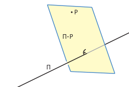
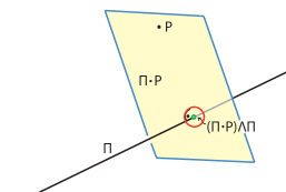
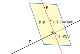
Figure 1: Solution of the exercise in PGA.

Things become even less satisfactory when one attempts to implement euclidean isometries. The authors acknowledge that using the non-degenerate metric, it is impossible to express euclidean translations as sandwich operators (§11.8 of [DFM07]). This leads to the conclusion:

The main problem with using the metric of $\mathbb{R}^{n+1}$ is that you cannot use it directly to do Euclidean geometry, for it has no clear Euclidean interpretation.

The foregoing quote is a good motivation for the next section, where we attempt to clarify the situation by differentiating various meanings of $\mathbb{R}^{n}$ and “euclidean”.

4.1.2 Three meanings of $\mathbb{R}^{n}$

The symbol $\mathbb{R}^{n}$ occurs 5 times in the two short quotes of the above section, grounds for asking what exactly it means. We can in fact distinguish at least three different meanings:

1. Vector space. In this form, $\mathbb{R}^{n}$ represents the vector space used to define real projective space $\mathbb{R}{P^{n-1}}$. It is an $n$-dimensional linear space with an addition operation, real scalar multiplication, and distributive law, but without inner product. One can develop a theory of linear mappings between such spaces, and from this, the dual vector space $\mathsf{V}^{*}$. The evaluation map $\mathbb{R}^{n}\otimes(\mathbb{R}^{n})^{*}\rightarrow\mathbb{R}$ of a vector and a dual vector (linear functional), often written $\langle\mathbf{v},\mathbf{\mu}\rangle:=\mathbf{\mu}(\mathbf{v})$ is sometimes confused with an inner product. We recommend using the terminology ($n$-dimensional) $\mathsf{V}$ for this meaning of $\mathbb{R}^{n}$, whenever possible. See [Gre67a], Chapter 1-2 for details.

2. Inner product space. One begins with a vector space and adds an inner product between pairs of vectors, which is a symmetric bilinear form on the vector space. This produces an inner product space. When the form is positive definite, it’s called a euclidean inner product space. We recommend retaining the use of $\mathbb{R}^{n}$ for this meaning. Consult [Gre67a], Chapter 7 for details on inner product spaces.

3. Euclidean space. This is a simply-connected metric space, of constant curvature 0, homeomorphic to $\mathbb{R}^{n}$ but equipped with the Euclidean distance function (discussed for example in [Gun11a], Chapter 4) between its points. We recommend using the notation $\mathbf{E}^{n}$ for this space. The points of $\mathbf{E}^{n}$ are in a 1:1 correspondence to the vectors of $\mathbb{R}^{n}$ (the origin of $\mathbf{E}^{n}$ maps to the zero vector of $\mathbb{R}^{n}$), but $\mathbf{E}^{n}$ is not a vector space, and the inner product discussed in the previous item has, a priori, nothing to do with the measurement of distances in $\mathbf{E}^{n}$.

Armed with these three different meanings which sometimes are attached to the same symbol $\mathbb{R}^{n}$, along with two meanings of euclidean (depending on whether one is in the vector space or the projective setting), let’s return to the discussion of the homogeneous model.

4.1.3 Rephrasing using the differentiated notation

When we apply this differentiated terminology and what we learned about the Cayley-Klein construction of metric spaces to the initial quote from [DFM07], we arrive at the following:

…[the homogeneous model] embeds $\mathbf{E}^{n}$ in a real vector space $\mathsf{V}$ of dimension $n+1$ and then uses the algebra of $\mathsf{V}$ to represent the elements of $\mathbf{E}^{n}$ in a structured manner.

In this form, $\mathbb{R}^{n}$ no longer occurs: there is no longer a given real vector space nor inner product, implied by the original definition. Consequently, one can use this modified description as a starting point for the search for the correct choice of Cayley-Klein space; we have sketched above how one arrives at the dual vector space $\mathsf{V}=(\mathbb{R}^{n+1})^{*}$ with signature $(n,0,1)$, yielding the algebra $\mathbf{P}(\mathbb{R}^{*}_{n,0,1})$.

To sum up: this confusion of the three meanings of $\mathbb{R}^{n}$ and two meanings of euclidean means that many of the objections to “the” homogeneous model appear in the light of the foregoing discussion as legitimate complaints against using the wrong vector space or the wrong signature to model euclidean geometry. In the next section we turn to consider if there are other choices which yield better results.

5 Homogeneous models using a degenerate metric

Faced with the difficulties ensuing on the use of the non-degenerate metric, [DFM07], p. 314, states:

We emphasize that the problem is not geometric algebra itself, but the homogeneous model and our desire to use it for euclidean geometry. It will be replaced by a much better model for that purpose in Chapter 13 [the conformal model - cg].

In fact, what the authors of [DFM07] have shown is that a homogeneous model with non-degenerate metric is “the problem” – recall that the use of degenerate metrics was rejected as inconvenient. Hence it remains to be seen whether a PGA based on a degenerate metric, such as $\mathbf{P}(\mathbb{R}^{*}_{n,0,1})$, could provide a faithful model for euclidean geometry. We now turn to an analysis of three common objections to the use of such a degenerate metric.

5.1 Objection 1: lack of covariance

Covariance has a variety of meanings related to the behavior of maps and coordinate systems; in our context, it is equivalent to the existence of sandwich (or versor) implementations of the euclidean group $E(n)$ ([DFM07], p. 369). That such versors exist for the even subalgebra of $\mathbf{P}(\mathbb{R}^{*}_{3,0,1})$ (and the associated Spin group) follows from its isomorphism with the biquaternions mentioned above in Sect. 3.8.1. The extension to the full algebra (and the associated Pin group) is straightforward and is described in [Gun11b], §15.4.2, §15.5.4.

One can gain a different impression, however, from some of the current literature. For example, [Li08], p. 11, identifies the Clifford algebra $\mathbf{P}(\mathbb{R}_{n,0,1})$ (in our notation) as the appropriate algebra for euclidean geometry. It focuses on the case of $n=3$ and remarks on the isomorphism of the dual quaternions with the even subalgebra. This leads to the remark:

However, the dual quaternion representations of primitive geometric objects such as points, lines, and planes in space are not covariant. More accurately, the representations are not tensors, they depend upon the position of the origin of the coordinate system irregularly.

In the first place, the proper algebra for euclidean geometry is not $\mathbf{P}(\mathbb{R}_{n,0,1})$ but the dual version $\mathbf{P}(\mathbb{R}^{*}_{n,0,1})$ (see above, Sect. 3.7.1). This confusion is perhaps due to the fact that the dual quaternions are isomorphic to the even sub-algebra of both these geometric algebras (Sect. 3.8.1 above). Furthermore, as discussed above in Sect. 2.2.2, the dual quaternion representation of points and planes is not the same as the representation of points and planes in these geometric algebras: the dual quaternion representation has irregularities not exhibited by the geometric algebra representation due to the fact there there is no natural representation for points and planes within the algebra. These irregularities however have to do with the form the sandwich operators take and do not effect the covariance of the representation. We are aware of no grounds for the claim made here that the dual quaternion representations are not covariant. It might be due to mixing up the two algebras $\mathbf{P}(\mathbb{R}_{n,0,1})$ and $\mathbf{P}(\mathbb{R}^{*}_{n,0,1})$ in the calculation, since each provides, taken for itself, covariant representations for their respective isometry group.

Readers who would like to confirm the claimed covariance for themselves, and do not have access to [Gun11b] or [Gun11a] are referred to Appendix A, which provides a detailed discussion of the versors of $\mathbf{P}(\mathbb{R}^{*}_{2,0,1})$ and their associated sandwich operators.

5.2 Objection 2: lack of duality

Another common objection to the use of degenerate metrics is often expressed in terms of a “lack of duality”. Consider the following quote from [HLR01], an article often associated with the birth of modern CGA ([DFM07], §13.8):

Any degenerate algebra can be embedded in a non-degenerate algebra of larger dimension, and it is almost always a good idea to do so. Otherwise, there will be subspaces without a complete basis of dual vectors, which will complicate algebraic manipulations.

As with the case of euclidean above, there are multiple meanings for the term dual in the literature which must be carefully differentiated. Here there are at least two distinct meanings:

1. The ability to calculate the regressive product. As shown in Sect. 3.4, for this operation one only requires the dual coordinates of a geometric entity, and this is provided in a non-metric way by Poincaré duality in the exterior algebra, or by the shuffle product.

2. The effect of multiplication by the pseudoscalar: $\Pi:\Pi(\mathbf{X}):=\mathbf{X}\mathbf{I}$. The action of $\Pi$ on the underlying projective space is known in classical projective geometry as the polarity on the metric quadric, that is, a correlation (maps points to hyperplanes and vice-versa) that maps a point to its orthogonal hyperplane with respect to the inner product encoded in the quadric, and vice-versa. When the metric is non-degenerate, then $\mathbf{I}^{2}=\pm 1$, and the polarity is a grade-reversing algebra bijection which is a vector-space isomorphism on each grade, and whose square is the identity. In this case, one can define the regressive product (analogously to the use of Poincaré duality in Sect. 3.4):

   $$\mathbf{X}\wedge\mathbf{Y}:=\Pi(\Pi(\mathbf{X})\vee\Pi(\mathbf{Y}))$$

We recommend that the term polarity be adapted also in geometric algebra for pseudoscalar multiplication, to distinguish it from the previous non-metric meaning of duality. So that, in the above quote, one would speak of the polar basis instead of the dual basis. The term dual basis would be reserved for the result of the dual coordinate map $\mathbf{J}$.

The implicit use of the metric to calculate the regressive product has a long tradition, going all the way back to Grassmann and continuing up to [HZ91], an influential modern article devoted to doing projective geometry using geometric algebra; its continued use of $\Pi$ for the regressive product – despite the absence of a natural metric for projective geometry – appears to have cemented the misunderstanding described here. As a result, in the above quote as well as other popular texts ([DFM07], [Per09], [DL03]) one might falsely gain the impression that a non-degenerate metric must be used to implement the regressive product, as few or no details of an alternative are provided. But in the absence of an invertible pseudo-scalar, one always has access to Poincaré duality. Hence this objection to PGA cannot be sustained.

5.3 Objection 3: Absence of invertible pseudoscalar

[Li08], also p. 11, raises a further (related) objection to the use of a degenerate metric:

Because the inner product in $\mathbb{R}_{n,0,1}$ is degenerate, many important invertibilities in non-degenerate Clifford algebras are lost.

We have discussed the invertibility of $\mathbf{I}$ as a condition for duality above in Objection 2, and shown that there are other means to implement duality. It is true that many formulas in the GA literature tend to be given in terms of $\mathbf{I}^{-1}$ rather than $\mathbf{I}$. But in the cases we are familiar with, it is also possible to use $\mathbf{I}$ instead, perhaps at the cost of a more complicated expression for the sign. For example, [Hes10] defines the dual (our polar!) of a multivector $A^{*}:=A\mathbf{I}^{-1}$ and shows then that the inner and outer products obey the relation: $a\cdot A^{*}=(a\wedge A)^{*}$. If instead one defines $A^{*}:=A\mathbf{I}$, the stated relation remains true, and valid for any pseudoscalar.

Experience leads us, in fact, to a very different view of the non-invertible pseudoscalar: it has proved to be an advantage, since it faithfully represents the metric relationships within euclidean geometry. The calculation from Sect. 4.1.1 provides a good example. Consider the sub-expression ${\mathbf{\Pi}}\cdot\mathbf{P}$. Letting the point $\mathbf{P}$ move freely, one obtains a set of parallel planes ${\mathbf{\Pi}}\cdot\mathbf{P}$ which all have the same polar point $({\mathbf{\Pi}}\cdot\mathbf{P})\mathbf{I}$, the ideal point of the line ${\mathbf{\Pi}}$. For invertible pseudo-scalars, however, the polar points of distinct planes are distinct. Or, recall the discussion of the special role of $\mathbf{e}_{0}$ in the solution in Sect. 4.1.1: it does not appear in the simpler PGA formula, since in PGA, $\mathbf{P}\mathbf{I}=\mathbf{\omega}_{P}$ for all normalized $\mathbf{P}$, while in the elliptic metric this is only true for $\mathbf{P}=\mathbf{e}_{0}$.

6 Comparison: A feature-set for “doing geometry”

Having sketched its mathematical lineage dating back to Klein and Clifford, and disposed of a series of modern objections which have been raised against it, the reader is hopefully convinced that euclidean PGA deserves the title of “standard” or “classical” homogeneous model of euclidean geometry. We are now prepared to compare it to the conformal model, CGA. As a basis for this comparison, we rely on a recent tutorial on the conformal model [Dor11]. This tutorial describes the challenge of “doing geometry” on a computer, a challenge which matches well with the chosen task we set out at the beginning of the article, so we use this tutorial as a basis for a first comparison of the two algebras. The tutorial lists seven “tricks” and three “bonuses” which the conformal model offers in this regard. We list them here:

1. Trick 1: Representing euclidean points in Minkowski space.

2. Trick 2: Orthogonal transformations as multiple reflections in a sandwiching representation.

3. Trick 3: Constructing elements by anti-symmetry.

4. Trick 4: Dual specifications of elements permits intersection.

5. Bonus: The elements of euclidean geometry as blades.

6. Bonus: Rigid body motions through sandwiching.

7. Bonus: Structure preservation and the transfer principle.

8. Trick 5: Exponential representation of versors.

9. Trick 6: Geometric calculus.

10. Trick 7: Sparse implementation at compiler level.

How does $\mathbf{P}(\mathbb{R}^{*}_{n,0,1})$ stand with respect to these features? In fact, it offers offers all the ten features listed. Some slight editing is required to “translate” to PGA; for example, Trick 1 has to be rephrased as “Representing euclidean points in projective space”. Duality (trick 4) is implemented in a non-metric way in our homogeneous model, and is used to represent join, not intersection. There are naturally some elements of euclidean geometry which cannot be represented as blades in PGA (bonus 1), such as point pairs and spheres. But the basic flat elements belonging to classical euclidean geometry are present: points, lines, and planes; and these are the ones belonging to the chosen task. We return to the richer class of primitives in CGA in Sect. 8 below.

One immediate corollary is that euclidean PGA ($\mathbf{P}(\mathbb{R}^{*}_{3,0,1})$) is the smallest known algebra that can model Euclidean transformations in a structure-preserving manner, a distinction sometimes claimed for CGA ([DFM07], p. 364). The importance of this result will become more apparent in the next section, which turns to a practical comparison of the two models.

7 Comparison: practical issues

Given the same feature set in these algebras, we shift our comparison to more practical considerations for the chosen task.

7.1 Complexity

The point $\mathbf{x}=(x,y,z)\in\mathbf{E}^{3}$ receives coordinates $(x,y,z,1)$ in PGA and $(1,x,y,z,\frac{1}{2}\|\mathbf{x}\|^{2})$ in CGA. The last coordinate is clearly non-linear function of the original ones. This standard representation is sometimes called the zero radius sphere (ZRS) representation of points in CGA. Also note, that as a result of having 1 more dimension, CGA also has twice the number of dimensions as PGA.

A more serious effect of the non-linear embedding of this representation, is that flat euclidean geometric configurations have to be represented and calculated as intersections of linear configurations with the null sphere of $\mathbf{P}(\mathbb{R}_{n+1,1,0})$. For example, if you want to subdivide a polygon in PGA, linear interpolation will preserve the flatness of the polygon; in the ZRS representation of CGA, you have to follow linear interpolation with a projection back onto the null sphere or devise other interpolation methods. As mentioned above in Sect. 3.8.2, one can alternatively use the flat representation in CGA, which is essentially the same as PGA. But to access the distinctive features of CGA (such as the distance function via the inner product) you have then to convert from the flat back to the ZRS representation, leading to the conclusion that one cannot in this way avoid the consequences of the non-linear embedding.

In general, any computation applied to a geometric primitive in the standard CGA representation risks moving off the null sphere, so potentially each step has to be checked against an error tolerance and corrected. PGA does not suffer from this difficulty, since all coordinates represent valid euclidean or ideal elements. Related problems arise with differential equations, as the next section shows.

7.2 Numerical analysis and differential equations

Consider the example of the euclidean equations of motion for a rigid body. (In PGA, for $n=3$, these are the biquaternion ODE’s given above in Sect. 2.2.) As with any ODE, the difficulty of solving the ODE is directly connected with how the space of valid solutions sits inside the full space of possible solutions; the smaller the co-dimension of the former in the latter, the easier the solution process is; see for example the discussion above in Sect. 2.1.1 regarding the advantages of the quaternion representation of rigid body motion over the matrix one. This difficulty is acknowledged in a recent article on 3D euclidean rigid body motion in the conformal model ([LLD11], §1.3.1):

… The idea here is to work in an overall space that is two dimensions higher than the base space, using the usual conformal Euclidean setup. The penalty for doing this, i. e., using a Euclidean setup, is that the number of degrees of freedom is not properly matched to the problem in hand, and we have to introduce additional Lagrange multipliers to cope with this. [our italics]

How do the two algebras compare in this regard? In both, the space of valid solutions for the Euler equations of rigid body motion consists of a euclidean bivector (in the Lie algebra $\mathfrak{e}(3)$) plus a euclidean rotor (in the Lie group $E(3)$); each is 6D, so the space of valid solutions is 12-dimensional. In the case of CGA, the full space of possible solutions is 26-dimensional (10D bivector and 16D even subalgebra). Here the co-dimension is 14, larger than the solution space itself, forcing the use of Lagrange multipliers. In contrast, the full solution space in PGA is 14-dimensional (6D bivector and 8D even subalgebra). Normalizing the rotor in PGA to have unit norm brings the solution back onto the valid solution space and provided reliable results for the extensive simulations in [Gun11a], Ch. 12), although the use of a Lagrange multiplier for the same purpose in the PGA case should be investigated. Given the availability of a fast and reliable PGA solution with minimal need for Lagrange multipliers, the question naturally arises, what advantages does the CGA approach to rigid body mechanics offer in compensation?

7.3 Kinematics, rigid body mechanics, and classical screw theory

As we noted above, PGA contains within it the biquaternions and their elegant representation of 3D euclidean kinematics and rigid body mechanics. This is essentially also the content of the screw theory of Robert Ball [Bal00]. As a result, all the features of these theories are included in PGA as a “native” element. [Hes10], on the other hand, envisions CGA as a means to “rejuvenate” classical screw theory. It would be worthwhile to compare the two approaches to screw theory with regard to such criteria as compactness of expression, practicality, and comprehensibility. For example, screw theory is built upon line geometry in $\mathbb{R}{P^{3}}$, which in turn is built upon Plücker coordinates for lines (bivectors). As noted above, these coordinates are native to PGA, but have to be extracted from the 10-dimensional coordinates of bivectors in CGA using the so-called conformal split ([Hes10], §VII).

7.4 Learning curve

The simplicity of the PGA representation leads to considerable savings in explaining the model, a significant advantage when considering the unfamiliarity of the underlying concepts. Since CGA is embedded in the hyperbolic PGA ($\mathbf{P}(\mathbb{R}^{*}_{n+1,1,0})$), learning the projective model is a natural step towards understanding the conformal model, but not vice-versa. From a pedagogical point of view, PGA forms a natural transition step between VGA and CGA. (A vector geometric algebra, or VGA for short, is a geometric algebra whose elements are interpreted as elements of a vector space, rather than projective space. )

8 Roundness and CGA

We have established that for the chosen task, PGA exhibits a series of practical advantages. Most of these can be arise from the contrast between, on the one hand, the flat embedding of $\mathbf{E}^{n}$ in $\mathbb{R}{P^{n}}$ in PGA and, on the other, the curved embedding of $\mathbf{E}^{n}$ within $\mathbb{R}{P^{n+1}}$ in CGA. We could say that the “roundness” of CGA is a liability when one is restricted to flat primitives. There is however another “roundness” in CGA that, for some euclidean applications, compensates for these liabilities: euclidean spheres are represented as points in CGA and can be manipulated on the same level as traditional flat primitives: points, lines, and planes. The restriction to spheres of radius 0 yields the curved model of $\mathbf{E}^{n}$ which has formed the basis of the comparison up to now. Removing the restriction to traditional flat primitives yields a powerful geometric toolkit ideally suited for many euclidean tasks where spheres (or conformal maps, see Sect. 3.8.2) play an intrinsic role ([DFM07], Ch. 14). There are a number of application areas, from optimization to robotics, whose problem settings do exhibit this close connection to sphere (or conformal) geometry. See, for example, [Dor14].

Users choosing between PGA and CGA are therefore advised to carefully weigh the advantages and disadvantages of the “roundness” of CGA in their decision. On the one side are the advantages of having a direct, powerful representation of spheres; on the other hand, are the disadvantages (discussed above) arising from the embedding of euclidean space itself as a sphere in a higher-dimensional projective space (the null sphere of $\mathbf{P}(\mathbb{R}_{n+1,1,0})$). Hence, if there is no intrinsic need for sphere geometry, as is the case for applications based on flat geometry, classical kinematics and rigid body mechanics, then the disadvantages listed in Sect. 7 can be expected to outweigh the advantages; if spheres form an essential geometric primitive, CGA is probably the right tool for the job. In between there’s much room for further research and development on how the strengths and weaknesses of the two approaches can be optimally combined.

9 Conclusion

We have reviewed important concepts from $19^{th}$ century mathematics, and clarified a set of fundamental terms, including homogeneous model, euclidean, $\mathbb{R}^{n}$, and duality, which are key to a correct understanding of how geometric algebra can be applied to doing euclidean geometry. On this basis, we have established that the dual projective geometric algebra $\mathbf{P}(\mathbb{R}^{*}_{n,0,1})$ deserves the title of “standard” homogeneous model for euclidean geometry. We have shown that it exhibits all the attractive features with respect to doing euclidean geometry which modern geometric algebra users expect, and is the smallest such algebra. Furthermore, in regard to practical considerations for the chosen task, we have found that it exhibits advantages over the higher-dimensional CGA, which remains the tool of choice for applications making essential use of spheres or conformal maps. For $n=3$, the most popular case, the fact that $\mathbf{P}(\mathbb{R}^{*}_{3,0,1})$ is built atop the biquaternions, William Clifford’s “other” great discovery (besides geometric algebra), means that users already familiar with the biquaternions are well-positioned to acquire PGA skills quickly.

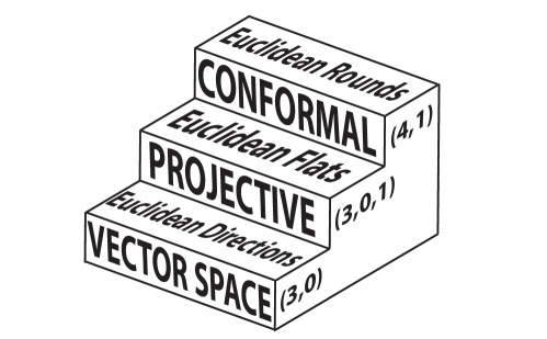
Figure 2: Progression of geometric algebras for euclidean geometry.

One area of concern for all practitioners of geometric algebra, regardless of specialization, is the slow rate at which geometric algebra has been adopted into the university curriculum (see [DL11], p. vi). We believe that the foregoing comparison can make a significant contribution to a solution of this challenge. PGA and CGA are not directly competitive, any more than automobiles and airplanes are directly competitive. As the previous section hopefully indicates, each has their proper, interdependent place in the geometric algebra ecosystem. Pedagogically, $\mathbf{P}(\mathbb{R}^{*}_{n,0,1})$ provides a natural stepping-stone (the “automobile”) between the $n$-dimensional vector space algebra $\mathbb{R}_{n,0,0}$ (the “bicycle” of the GA world, aka VGA) and the $(n+2)$-dimensional CGA (the “airplane”). See Fig. 2. In light of Sect. 7.4, we can expect that PGA will be accessible to a significantly larger pool of students than currently is the case with CGA. This will also simplify the teaching of CGA since, as remarked above, CGA is built on top of PGA. We suggest that the PGA treatment of euclidean geometry, kinematics, and mechanics is exactly what is needed to solve the GA adoption problem by providing a non-trivial link between VGA and CGA, just as the automobile fits between the bicycle and the airplane.

Thus, these two algebras exist not in a competitive but a complementary relationship. The nature of this complementarity was already expressed by Johannes Kepler – perhaps the first scientist to apply mathematics in a modern way to the study of the outer world – when he wrote ([Kep19]):

…God, in his measureless wisdom, selected at the very beginning the straight and the curved, in order with them to imprint into the world the divinity of the Creator… In this way the most Wise devised the extensive world, whose whole being is encompassed between the two contrary principles, the straight and the curved.

Rounding off our article in Kepler’s style, we might say that God has given us PGA to understand and to master the world of the straight, while he has given us CGA to do the same for the world of the round.

10 Acknowledgements

The author would like to thank the third reviewer for his detailed comments, which led to numerous improvements in the article.

Appendix A Versors for the euclidean plane.

Begin with two normalized 1-vectors $\mathbf{a}$ and $\mathbf{b}$ in $\mathbf{P}(\mathbb{R}^{*}_{2,0,1})$, each representing a line in the euclidean plane and assume that they meet in a euclidean point $\mathbf{P}$, i. e., $\mathbf{a}\wedge\mathbf{b}=\mathbf{P}\neq 0$. We show that $R_{\mathbf{a}}(\mathbf{b})$, the reflection of the line $\mathbf{b}$ in the line $\mathbf{a}$, is given by $\mathbf{a}\mathbf{b}\mathbf{a}$.

Using basic facts of elementary geometry, it’s not hard to show that $\mathbf{x}:=R_{\mathbf{a}}(\mathbf{b})$ can be uniquely characterized as the line which passes through $\mathbf{P}$, the intersection of $\mathbf{a}$ and $\mathbf{b}$, and whose oriented angle to $\mathbf{a}$ is equal but opposite to the angle $\mathbf{b}$ makes to $\mathbf{a}$. The derivation of the signature $(2,0,1)$ in Sect. 3.5.1 allows us to translate these conditions into the language of the geometric product in $\mathbf{P}(\mathbb{R}^{*}_{2,0,1})$: $\mathbf{x}\cdot\mathbf{a}=\mathbf{b}\cdot\mathbf{a}$ and $\mathbf{x}\wedge\mathbf{a}=-\mathbf{b}\wedge\mathbf{a}$. First note that $\mathbf{a}\mathbf{b}\mathbf{a}$ is a 1-vector (a line), since the three arguments are not linearly independent, so their wedge is 0. Is it the desired line? Substituting $\mathbf{a}\mathbf{b}\mathbf{a}$ for $\mathbf{x}$ in the first condition and applying symmetry of ($\cdot$) and the normalization condition $\mathbf{a}^{2}=1$ yields

$$\mathbf{x}\cdot\mathbf{a} =\dfrac{1}{2}(\mathbf{a}\mathbf{b}\mathbf{a}^{2}+\mathbf{a}^{2}\mathbf{b}\mathbf{a})$$

$$=\dfrac{1}{2}(\mathbf{a}\mathbf{b}+\mathbf{b}\mathbf{a})$$

$$=\mathbf{a}\cdot\mathbf{b}=\mathbf{b}\cdot\mathbf{a}$$

And the second condition proceeds similarly, using the anti-symmetry of $\wedge$:

$$\mathbf{x}\wedge\mathbf{a} =\frac{1}{2}(\mathbf{a}\mathbf{b}\mathbf{a}^{2}-\mathbf{a}^{2}\mathbf{b}\mathbf{a})$$

$$=\frac{1}{2}(\mathbf{a}\mathbf{b}-\mathbf{b}\mathbf{a})$$

$$=-\mathbf{b}\wedge\mathbf{a}$$

Hence, $\mathbf{x}$ fulfills the conditions and is, therefore, the reflection of the line $\mathbf{b}$ in the line $\mathbf{a}$. We leave it as an exercise for the reader to verify that this argument remains true when $\mathbf{a}$ and $\mathbf{b}$ are parallel (i. e., $\mathbf{P}$ is ideal). A further exercise: $\mathbf{a}\mathbf{P}\mathbf{a}$ is the reflection of a euclidean point $\mathbf{P}$ in the line $\mathbf{a}$. The tireless reader can then extend this result to the full euclidean isometry group by applying the well-known result that all isometries can be factored as a sequence of reflections in euclidean lines. Such a sequence of reflections yields, in the algebra, a versor $\mathbf{R}$ consisting of the product of the corresponding 1-vectors. When the 1-vectors are normalized, then so is the resulting versor, which then belongs to the rotor group, and one obtains the sandwich operation associated to this rotor: $\mathbf{R}\mathbf{X}\widetilde{\mathbf{R}}$. Nothing in this proof essentially depends on the dimension $n=2$, it generalizes directly and establishes the claim that the versor representation of the isometry group in $\mathbf{P}(\mathbb{R}^{*}_{n,0,1})$ works as advertised.

References

- [Bal00] Robert Ball. A Treatise on the Theory of Screws. Cambridge University Press, Cambridge, 1900.
- [BCDK00] Eduardo Jose Bayro-Corrochano, D., and D. K hler. Motor algebra approach for computing the kinematics of robot manipulators. J. Robotic Syst., 17:495–516, 2000.
- [Bla42] Wilhelm Blaschke. Nicht-euklidische Geometrie und Mechanik. Teubner, Leipzig, 1942.
- [Cli73] William Clifford. A preliminary sketch of biquaternions. Proc. London Math. Soc., 4:381–395, 1873.
- [DFM07] Leo Dorst, Daniel Fontijne, and Stephen Mann. Geometric Algebra for Computer Science. Morgan Kaufmann, San Francisco, 2007.
- [DL03] Chris Doran and Anthony Lasenby. Geometric Algebra for Physicists. Cambridge University Press, Cambridge, 2003.
- [DL11] Leo Dorst and Joan Lasenby, editors. Guide to Geometric Algebra in Practice. Springer London, 2011.
- [Dor11] Leo Dorst. Tutorial appendix: Structure preserving representation of euclidean motions through conformal geometric algebra. In Leo Dorst and Joan Lasenby, editors, Guide to Geometric Algebra in Practice, pages 435–453. Springer London, 2011.
- [Dor14] L. Dorst. Total least squares fitting of k-spheres in n-d euclidean space using an (n+2)-d isometric representation. J of Mathematical Imaging and Vision, pages 1–21, 2014.
- [Gre67a] W. H. Greub. Linear Algebra. Springer, 1967.
- [Gre67b] W. H. Greub. Multilinear Algebra. Springer, 1967.
- [Gun11a] Charles Gunn. Geometry, Kinematics, and Rigid Body Mechanics in Cayley-Klein Geometries. PhD thesis, Technical University Berlin, 2011. http://opus.kobv.de/tuberlin/volltexte/2011/3322.
- [Gun11b] Charles Gunn. On the homogeneous model of euclidean geometry. In Leo Dorst and Joan Lasenby, editors, A Guide to Geometric Algebra in Practice, chapter 15, pages 297–327. Springer, 2011.
- [Gun11c] Charles Gunn. On the homogeneous model of euclidean geometry: Extended version. http://arxiv.org/abs/1101.4542, 2011.
- [Gun16] Charles Gunn. Geometric algebras for euclidean geometry. Advances in Applied Clifford Algebras, pages 1–24, 2016.
- [Hes10] David Hestenes. New tools for computational geometry and rejuvenation of screw theory. In Eduardo Jose Bayro-Corrochano and Gerik Scheuermann, editors, Geometric Algebra Computing in Engineering and Computer Science, pages 3–35. Springer, 2010.
- [HLR01] David Hestenes, Hongbo Li, and Alyn Rockwood. A unified algebraic approach for classical geometries. In Gerald Sommer, editor, Geometric Computing with Clifford Algebra, pages 3–27. Springer, 2001.
- [HZ91] David Hestenes and Renatus Ziegler. Projective geometry with clifford algebra. Acta Applicandae Mathematicae, 23:25–63, 1991.
- [Kep19] Johannes Kepler. Harmonices Mundi LIbri V. Linz, 1619.
- [Kle26] Felix Klein. Vorlesungen Über Nicht-euklidische Geometrie. Chelsea, New York, 1926. (Original 1926, Berlin).
- [Kow09] Gerhard Kowol. Projektive Geometrie und Cayley-Klein Geometrien der Ebene. Birkhauser, 2009.
- [Li08] Hongbo Li. Invariant Algebras and Geometric Reasoning. World Scientific, Singapore, 2008.
- [LLD11] Anthony Lasenby, Robert Lasenby, and Chris Doran. Rigid body dynamics and conformal geometric algebra. In Leo Dorst and Joan Lasenby, editors, Guide to Geometric Algebra in Practice, chapter 1, pages 3–25. Springer, 2011.
- [Per09] Christian Perwass. Geometric Algebra with Applications to Engineering. Springer, 2009.
- [Sel00] Jon Selig. Clifford algebra of points, lines, and planes. Robotica, 18:545–556, 2000.
- [Sel05] Jon Selig. Geometric Fundamentals of Robotics. Springer, 2005.
- [Stu03] Eduard Study. Geometrie der Dynamen. Tuebner, Leibzig, 1903.
- [vM24] Richard von Mises. Die Motorrechnung: Eine Neue Hilfsmittel in der Mechanik. Zeitschrift für Rein und Angewandte Mathematik und Mechanik, 4(2):155–181, 1924.
- [Zie85] Renatus Ziegler. Die Geschichte Der Geometrischen Mechanik im 19. Jahrhundert. Franz Steiner Verlag, Stuttgart, 1985.