Orbital magnetism of coupled bands models
Abstract
We develop a gauge-independent perturbation theory for the grand potential of itinerant electrons in two-dimensional tight-binding models in the presence of a perpendicular magnetic field. At first order in the field, we recover the result of the so-called modern theory of orbital magnetization and, at second order, deduce a new general formula for the orbital susceptibility. In the special case of two coupled bands, we relate the susceptibility to geometrical quantities such as the Berry curvature. Our results are applied to several two-band – either gapless or gapped – systems. We point out some surprising features in the orbital susceptibility – such as in-gap diamagnetism or parabolic band edge paramagnetism – coming from interband coupling. From that we draw general conclusions on the orbital magnetism of itinerant electrons in multi-band tight-binding models.
I Introduction
The magnetic response of itinerant electronic systems in the absence of spin-orbit coupling can be split in two different parts: spin and orbital contributions. The spin susceptibility is easily understood in terms of Pauli paramagnetism as it only depends on the density of states at the Fermi levelAshcroft . There is no essential difference between the case of free electrons and that of Bloch electrons. In the following, we therefore consider spinless electrons and focus on orbital magnetism of itinerant electrons. The study of the later begun with Landau Landau30 for free electrons, and continued with Peierls Peierls33 who took explicitly the effect of the periodic potential into account: he derived a formula which is valid in a one-band approximation (single band tight-binding model). After these pioneering works, a lot of effort has been put in trying to generalize the so-called Landau-Peierls (LP) formula to many-band systems Adams53 ; Hebborn60 ; Roth62 ; Wannier64 ; Misra69 with different approaches: effective multiband Hamiltonians, use of Bloch or Wannier functions, etc. The challenge was to tackle the case of coupled bands, the contribution of which cannot be treated separately. However, the resulting formulae were so complicated that any attempt of physical interpretation was vain, and a complete evaluation was in general impossible. Fukuyama Fukuyama71 first gave a very compact expression for the susceptibility in terms of Green’s functions using a slowly varying vector potential for a perfect periodic system. While his linear response formula gave interesting results (for example in bismuthFukuyama70 ), it seems to be incomplete for tight-binding systems as it does not recover the LP formula in the single-band limit. In the context of graphene, the Fukuyama formula was recently completed for the tight-binding model by Gomez-Santos and Stauber Gomez-Santos11 and anticipated by Koshino and Ando Koshino07 .
Graphene, first theoretically studied by Wallace Wallace47 and experimentally discovered sixty years later by Novoselov and Geim Novoselov04 , is a honeycomb lattice of carbon atoms that remains conducting despite its minimal thickness. It is essentially a strongly coupled two-band system that is ideally suited to test the prediction of orbital susceptibility formulae. The simplest tight-binding model describing graphene Wallace47 can actually be considered as a paradigmatic case of strong band coupling. Like bismuth, graphite is known for its huge diamagnetism which seems to be also experimentally observed in graphene Sepioni10 ; Nikolaev13 . McClure McClure56 derived such a property from graphene’s unusual Landau levels at half filling. He showed that, when the chemical potential is right at the Dirac point (usually at ), the susceptibility becomes infinitely diamagnetic as the temperature vanishes. This can not be recovered by the LP formula and is therefore a signature of interband effects on the magnetic response of graphene. However, McClure’s formula predicts a null susceptibility as soon as . This is not correct for at least two reasons. First, it violates an exact sumrule (see below). Second, Vignale Vignale91 showed quite generally that, in the vicinity of a saddle point in the dispersion relation (corresponding to a van Hove singularity in the density of states, which occurs in graphene at finite energy eV), the susceptibility should actually be infinitely paramagnetic and not zero. The Fukuyama formulaFukuyama71 correctly recovers the McClure diamagnetic peakFukuyama07 and the van Hove paramagnetism but fails to describe the exact chemical potential dependance of the tight-binding model, as we discuss below. The formula derived by Ref. [Gomez-Santos11, ] succeeds in giving the susceptibility of graphene for any value of the chemical potential (controlling the band filling) and a numerical approach done in Ref. [Raoux14, ] based on the energy spectrum of the honeycomb lattice in a magnetic field (graphene’s Hofstadter butterfly Rammal85 ) confirmed it.
In order to derive the orbital susceptibility, the authors of Ref. [Gomez-Santos11, ] use a gauge-dependent procedure in which they employ a trick to derive a continuous version of the tight-binding Hamiltonian. In particular, the derivation of the effective current operator seems ambiguous since different non-equivalent expressions can be found (even if the zero wavevector limit remains the same). Several recent works Savoie12 ; Chen11 ; Nourafkan14 ; Swiecicki14 derived a gauge-independent perturbation theory of the grand potential. Refs. [Chen11, ; Nourafkan14, ] restrict to the magnetization, and Ref. [Savoie12, ] gives a (rather elaborate) formula for the orbital susceptibility.
This paper presents a perturbation theory for independent particles (Sec. II) in terms of the magnetic field using Green’s functions which are explicitly gauge-independent Savoie12 ; the derivation presents a straightforward physical interpretation as it does not use a continuous limit. In addition, this method easily allows one to get both the magnetization – related to the first-order term in the magnetic field – and the orbital susceptibility as the second-order term. The expansion actually holds to any order in the magnetic field. In particular we recover (Sec. III) the formula of the magnetization in terms of the Berry curvature and the orbital magnetic moment, as obtained in the so-called modern theory of orbital magnetization Thonhauser11 ; Thonhauser05 ; Xiao05 . In Sec. IV, we present a new formula for the orbital susceptibility, see Eq. (24), and compare it to the different results listed in the introduction. In particular, it agrees with the formula of Ref. [Gomez-Santos11, ]. Next, we derive a convenient formula for the orbital susceptibility of two-band tight-binding models (see Eq. (30)), that we apply to several specific Hamiltonians (Sec. V) in order to gain insight on the importance of interband coupling. Equations (24) and (30) are the main results of this paper. Eventually, we give a general conclusion on orbital magnetism of coupled bands models in Sec. VI.
II General derivation
Motivation—
We restrict ourselves to 2D systems to simplify the algebra. In the presence of a magnetic field along the transverse axis , the grand canonical potential of a Fermi-Dirac gas of non-interacting electrons yields
| (1) |
where is the density of states (DoS) of the system (we use units such that the Boltzmann constant ). The quantities of interest are derivatives of the grand potential taken in the limit : the magnetization
| (2) |
and the orbital susceptibility ( in S.I. units)
| (3) |
which, via , only depend on derivatives of . is the sample area. In 2D, is homogeneous to a length. The DoS can be written in terms of the retarded Green’s function of the system
| (4) |
so that we will search for a perturbation theory of .
A useful tool in the following will be the magnetic sumrule: it can be shown (see Supplemental material of Ref. [Raoux14, ]) that
| (5) |
from which we deduce the sumrule relative to the susceptibility
| (6) |
This sumrule holds for any tight-binding model, provided the magnetic field only enters as a Peierls phase on the hopping amplitudes in the Hamiltonian (see below).
System—
Starting from a tight-binding Hamiltonian in real-space representation in the absence of a magnetic field:
| (7) |
where and are site indices, the magnetic field is taken into account by performing the Peierls substitution where
| (8) |
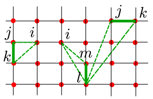
being a vector potential corresponding to a static uniform magnetic field. Let us define the quantity
| (9) |
If depends on the gauge, is gauge-independent using Stokes’ formula since it is proportional to the magnetic flux through the oriented triangle (cf. Fig. 1). Its explicit expression in Cartesian coordinates is
| (10) |
Perturbation theory—
The total Hamiltonian in a field reads
| (11) |
Let (resp. ) be the Green’s function relative to (resp. ). If one directly expands in powers of , one gets a gauge-dependent expression. A trickSavoie12 ; Chen11 to circumvent such a problem is to define a new “twisted” Green’s function by
| (12) |
then expand in terms of and finally reintroduce in order to recover a gauge-independent expression for the diagonal elements of .
One easily shows that
| (13) |
with
| (14) |
Eq.(13) gives:
| (15) |
Because the interesting part is the trace of , only the diagonal terms in Eq. (15) need to be considered. Let and denote the linear and quadratic terms in the magnetic field respectively. The expansion of Eq. (15) in gives
| (16) |
and
| (17a) | ||||
| (17b) | ||||
The diagonal quantities () only depend on gauge-independent variables; it is not the case of off-diagonal elements. Note that second-order expansion in contains first and second powers in the operator . The two terms Eqs. (17a) and (17b) are of order and are reminiscent of the Larmor (first order in ) and Van Vleck (second order in ) contributions, that are well-known in the magnetism of isolated atomsAshcroft
Using Eq. (10) and defining position operators and , and can be expressed in terms of commutators of , , and . To shorten the notations, if is an operator, (resp. ) will be denoted (resp. ); this notation will correspond to a derivative with respect to (resp. ) in the -space representation. The particular case where is the Hamiltonian yields the velocity operator . With these notations, Eqs. (16) and (19) become
| (18) |
and
| (19) |
The last term of Eq. (19) looks like the square of the first order correction. It corresponds to the Van Vleck term of atomic physics. The equality (and equivalently with ) will be useful to compute the commutators of the Green’s functions.
III Orbital Magnetization
In a perfect crystal, the set of Bloch functions diagonalizes the Hamiltonian. If is a Bloch function, eigenfunction of the Hamiltonian with eigenvalue , then is a periodic function with the periodicity of the lattice, and is an eigenfunction of with the same eigenvalue ( being the position operator in the definition of ). Using this basis, it is a little long but straightforward (cf. Appendix A) to recover from Eqs. (1, 2, 4, 18) the nowadays well-established formulaXiao05 ; Thonhauser05 for the magnetization
| (20) |
in terms of the Berry curvature and the magnetic moment along the axisChen11 ; Nourafkan14 :
| (21) | ||||
| (22) |
where is the Fermi function (implicitely depending on and ) and the projector from the Hilbert space to the state .
The above derivation can be straightforwardly extended to the case of a finite and disordered system described by a Hamiltonian . If we call a set of eigenstates and eigenvalues of , then equations corresponding to (20), (21) and (22) are obtained throught the substitutions , and . In addition, starting from Eq. (18), one could also derive the local orbital magnetization (see, e.g. [Bianco13, ]).
In a system that is time-reversal invariant, the spontaneous magnetization vanishes and one needs to go to the second order response in order to obtain orbital magnetism.
IV Orbital Susceptibility
We now derive a new formula for the orbital susceptibility. Starting from Eq. (19) and after some algebra (cf. Appendix B), one obtains:
| (23) |
should be understood as the -derivative of , . The general formula for the orbital susceptibility follows:
| (24) |
Equation (24) is the first main result of this paper. As for the orbital magnetization, the above formula is valid even if the system does not have translational symmetry such as molecules, ribbons or disordered systems. In the remaining of the present paper, we restrict to infinite crystals.
In the case of a single band, where the integration is performed over the first Brillouin zone (BZ), the last term (in parenthesis) in the trace of this formula vanishes and one immediately recovers the Peierls formulaPeierls33
| (25) |
with the energy spectrum. A detailed discussion on the use of the one-band LP formula is provided in Appendix C. Moreover, using a partial integration in Eq. (24), we recover another expression of the susceptibility obtained in Ref. [Gomez-Santos11, ](Eq. (3)):
| (26) |
Fukuyama’s formulaFukuyama71 is the first term in the trace of Eq. (26). Nevertheless, Fukuyama’s formula does not recover the LP result in the one-band case (see Fukuyama’s discussion of that point in Ref. [Fukuyama71, ] and our discussion in Appendix C). Actually, the Fukuyama formula does not work for tight-binding models that are not separable, i.e. such that , see [Gomez-Santos11, ; Koshino07, ]. In order to recover the LP formula, one needs to consider the full Eq. (26), as the two terms contribute in the one-band limit. In this regard, Eq. (24) is more adequate than Eq. (26) to such a comparison: indeed, the first two terms (quadratic in ) of the trace in Eq. (24) consist in a “generalized” version of Eq. (25), and if and commute with (a one-band Hamiltonian is a scalar), the last term vanish, and this directly leads to the LP formula. For this reason, Eq. (24) is preferred in the following.
The LP result is strictly valid only for a single band. However, it does contain interesting physics that is useful even when discussing two-band models with band coupling (see Appendix C). In the multi-band case, the LP formula can be trivially extended to an approximate “band by band” formulaFukuyama71
| (27) |
which neglects all interband effects. It will serve for comparison purposes below.
V Application to two-band models
V.1 Two-band formula
In this section, we derive a formula valid for two-band models with particle-hole symmetry, in order to illustrate as clearly as possible the effects of interband coupling on the magnetic response of a crystal.
For such models, the -space Hamiltonian matrix can be written where is the vector of Pauli matrices, and a 3-dimensional vector depending on the 2-dimensional vector . This Hamiltonian has two eigenvalues for each : with . They are associated to two eigenspaces defined by their projectors: , where is a unit vector on the sphere . The Hamiltonian reads . In this basis, and are diagonal and in particular: with . Interband coupling arises because derivatives of the Hamiltonian are not diagonal in this basis. For brevity, the -dependence will be implicit in the following except in definitions.
In Eq. (24), the trace is where the integration is performed over the first Brillouin zone (BZ), being the partial trace operator on the band index. We separate two different contributions:
| (28) | ||||
| (29) |
and qualitatively differ because is made of second-order derivatives of the Hamiltonian, but is only composed of first-order derivatives.
After some algebra (see Appendix D for details), the susceptibility can be written:
| (30) |
with a shorthand notation for and , are first and second derivatives of . We have also defined the quantities:
| (31) |
with and . The last quantity has been written in terms of the Berry curvature , which, in the particle-hole symmetric two-band case, is also related to the orbital magnetic moment Xiao10 ; Fuchs10 . We have used this expression to compute the susceptibility in various examples presented below.
Eq. (30) is the second main result of the present paper. It is a computable expression for numerical integration and is the starting point to discuss some examples in the next sections. Furthermore, the way it is written, each three parts verifies independently the susceptibility sumrule in Eq. (5). However, it is also possible to have expressions in which only and appear (and no longer ). This work will be presented elsewhereRaouxUnpublished . It is tempting to interpret terms proportional to as Fermi surface contributions and those proportional to as bulk Fermi sea contributions.
In the remaining part of the paper, we apply Eq. (30) to different two-band models in order to highlight some features in the orbital magnetic response linked to interband coupling.
V.2 Gapless Systems
V.2.1 Graphene
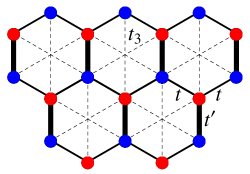
The honeycomb lattice is plotted in Fig. 2. We consider the usual model of graphene, i.e. the nearest-neighbor tight-binding model with hopping amplitude (corresponding to and in Fig. 2). The -space Hamiltonian can be written as withCastroNeto09
| (35) | ||||
| (39) |
in which () are the vectors linking a atom to its three nearest-neighbors (Fig. 2). From now on, we use units such that the nearest neighbor distance , and . We also introduce a convenient susceptibility scale (with typical values eV and Å, Å corresponding in 3D to . This is as large as orbital susceptibility gets in experiments, apart from superconductors).
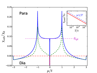
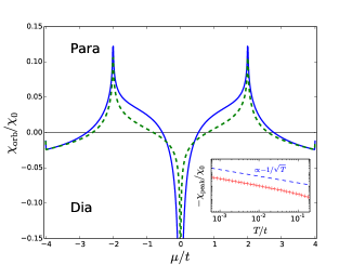
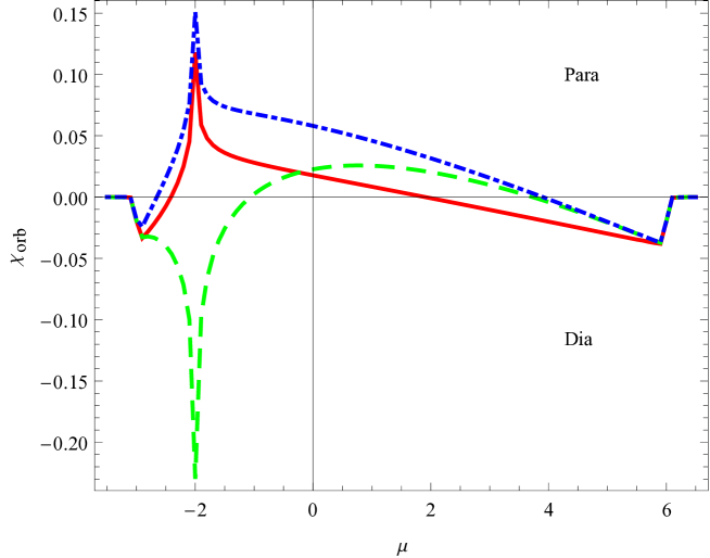
The total orbital susceptibility of graphene has already been derived by Gomez-Santos et al.Gomez-Santos11 but it deserves more discussion. Fig. 3 shows the susceptibility as a function of the chemical potential from Eq. (30). It coincides with Fig. 1 of Ref. [Gomez-Santos11, ]. The LP contribution and the McClure prediction are plotted as well. As found by McClureMcClure56 , the susceptibility diverges as at vanishing chemical potential:
| (40) |
The inset of Fig. 3 shows the result of our calculations at . The qualitative behavior in is verified, and it quantitatively agrees with McClure up to a constant paramagnetic correction independent of which we call the paramagnetic plateau. We found a lengthy analytical expression for this quantity in terms of an integral. Numerical quadrature gives
which is roughly five times the diamagnetism at the band edges. The numerical results at are well adjusted by with . We compared the result for to our numerical method based on the Hofstadter spectrum Raoux14 and found excellent quantitative agreement. Note that the two methods are completely different: one is a perturbative response formula, the other is non-perturbative and relies on an exact diagonalization of the Hamiltonian in a small but finite magnetic field.
When at , McClure predicted a vanishing susceptibility as Eq. (40) gives when . It appears that the strong diamagnetic contribution is only at , but we see on Fig. 3 that the paramagnetic plateau remains when .
At , we observe a diverging paramagnetic contribution, which corresponds to van Hove singularities in the DoS. Such orbital paramagnetism was discussed quite generally by VignaleVignale91 . The LP formula predicts this effect, as it is encoded in the DoS and the curvature of the spectrum (see Appendix C).
Finally, outside of the van Hove singularities (), the susceptibility is qualitatively described by the LP formula and converges in the edges of the spectrum () to the Landau diamagnetism of “quasi-free” electrons
| (41) |
with a band mass consistent with the quadratic approximation of the dispersion relation near . The diamagnetic peak and the paramagnetic plateau should be understood as the result of strong interband coupling between valence and conduction bands. This interband coupling decreases when increases, as revealed by a better agreement with the LP formula upon approaching the band edges. Note that the sumrule (Eq. (5)) is neither verified by the LP susceptibility, nor by the McClure formula alone, but is fulfilled by the total formula of Eq. (24).
If one is only interested in the susceptibility, one might be tempted to use a low-energy approximation. As a matter of fact, McClure partially succeeded in using this approach for graphene. With the low-energy Hamiltonian, he derived the associated Landau levels, and deduced the susceptibility by the Euler-MacLaurin formula. In a previous workRaoux14 , it has been shown that the sign of the susceptibility in a magnetic field is generally governed by the behavior of the first Landau level. Another low-energy technique, which will be used for comparison purposes in the following, is to compute the susceptibility using Eq. (30) and a linearised Hamiltonian near zero energy (namely the Dirac points for graphene). Appendix E gives some details for the case of graphene and recovers Eq. (40). The paramagnetic plateau is however not recovered by this method; it is a property coming from the full Hamiltonian, and which can not be found by a low-energy approach. A second-order approximation does not yield the plateau either. The plateau contribution comes from terms proportional to in Eq. (30). This result illustrates that the magnetic response can not be fully understood as a Fermi surface property (see, for example, the discussion in Ref. [Haldane04, )].
V.2.2 Pseudo graphene bilayer
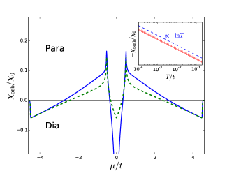
Bilayer graphene also has a gapless structure but with parabolic (instead of linear) band touching points. Although to be correctly described, bilayer graphene requires a Hamiltonian, the physics near the contact points is well-understood within a low-energy modelMcCann06 . We take a different route and choose a convenient tight-binding two-band toy-modelMontambaux12 , that reproduces the low-energy effective Hamiltonian of bilayer graphene near the band touchings. As a tight-binding model, it is compatible with the use of Eq. (30). Compared to Fig. 2, this toy-model takes into account nearest-neighbor hopping (as in graphene) and third-nearest-neighbors with a hopping amplitude . The Hamiltonian is given by with and
| (42) |
Fig. 4 presents the susceptibility of this model, which fulfils the susceptibility sumrule. The behavior should be similar to that of bilayer graphene (note, however, that this is not completely obvious as one of the main message of the present article is that orbital magnetism is not just a property of the Fermi surface but receives contributions from all the filled bands): there is a diamagnetic peak but with a logarithmic temperature scaling (inset of Fig. 4), different from the monolayer. The LP formula gives a finite contribution (of the Landau diamagnetism type) due to the parabolic behavior of the bands at zero energy.
A low-energy approach using the approximate Hamiltonian of bilayer graphene near yields
| (43) |
consistent with previous calculationsSafran84 ; Koshino07 , where is an ultraviolet energy cutoff of the order of magnitude of the interlayer coupling. It gives the validity limit of the 2-band approximation of the 4-band Hamiltonian. In particular, we find that . The inset of Fig. 4 confirms this scaling.
V.2.3 At the merging transition: semi-Dirac fermions
The last gapless system we investigate is an example of semi-Dirac electrons (quadratic-linear spectrum) in a strongly deformed honeycomb lattice described by the nearest-neighbor tight-binding model. If a uniaxial strain is applied to a graphene sheet (this is known as a quinoid deformation), it results in an anisotropy which phenomenologically induces two different values for the hopping amplitudes and Montambaux09 ; Montambaux09_prb (see Fig. 2). There is a critical point at case, where the two initial Dirac points exactly merge at a point of the Brillouin zone. This corresponds to a topological Lifshitz transition. Exactly at the transition, withDietl08
| (44) |
The corresponding low-energy spectrum (near the points) of this model is of the semi-Dirac type: it is quadratic in one reciprocal space direction (taken as ) and linear in the perpendicular () one. Surprinsingly, the LP formula predicts a diverging diamagnetic contribution at , eventhough the DoS vanishes. The exact orbital susceptibility is plotted in Fig. 5. It does show a diamagnetic divergence at zero chemical potential, but with a different temperature scaling than that predicted by the LP formula.
At , a low-energy analysis can be performed analytically to yield:
| (45) |
with the Euler function and . It confirms the diamagnetic divergence and the scaling. A similar behavior has been proposed previouslyBanerjee12 – albeit with a very different numerical prefactor – and based on an approximate one-band formula. This model gives a different example of the effect of interband coupling. In that case, it renormalizes the diverging susceptibility near the band touching. Note that, on a qualitative level, the LP formula does a reasonable job there.
V.2.4 Conclusion on gapless systems
We summarize the general behavior observed in all two-band gapless systems considered here: they all present a diamagnetic diverging susceptibility when the chemical potential is at the band touching energy. Note that this is not a general feature: in Ref. [Raoux14, ], we showed that in a 3-band gapless tight-binding model, the diverging susceptibility at the band touching points could be tuned from dia- to para-magnetic, without changing the zero-field energy spectrum. The tuning parameter only affects the zero-field eigenstates. This shows the importance of interband effects.
V.3 Gapped Systems
V.3.1 Boron nitride or “gapped graphene”
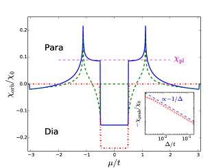
Consider a honeycomb lattice with a staggered on-site potential for and atoms corresponding to boron and nitrogen atoms, for example. This inversion symmetry-breaking opens a gap at the (ex-)Dirac pointsSemenoff84 . The Hamiltonian is the same as that of graphene albeit with instead of in Eq. (39). In the multiband LP formula, a full or empty band does not contribute to the total magnetic response, and thus a zero susceptibility is expected in any gap. Fig. 6 shows both the LP susceptibility and the result of Eq. (30) for boron nitride. A striking difference between the two graphs is the presence of a residual diamagnetism in the gap, even if the gap is large. Again, we interpret this observation as interband coupling even if the two bands are far away in energy. This result can be understood from the graphene case: the broadening of the peak by temperature is studied in the previous section; here the delta peak is broadened by the presence of another energy scale: namely the gap . Thus, one can guess that the susceptibility in the gap depends on the gap as . This is indeed verified by the inset of Fig. 6. More precisely, the value is the sum of two terms: the constant paramagnetic plateau for graphene and a McClure-like diamagnetic part. Using the linearised Hamiltonian of boron nitride in Eq. (30), the low-energy approach gives:
| (46) |
which looks like a “generalised McClure formula” for a non-vanishing gapNakamura07 ; Koshino10 . It converges towards Eq. (40) when .
While crossing the gap, the susceptibility suffers a discontinuity: it goes from dia- to paramagnetism. This is surprising: at a parabolic band edge, one would expect the susceptibility to converge to Landau’s diamagnetic value. The susceptibility outside of the gap is actually very similar to graphene’s. A null susceptibility outside of the gapNakamura07 ; Koshino10 is an artefact of the low-energy approach. When considered as a doped semiconductor, boron nitride has a very unusual behavior: near a parabolic band bottom (), it features orbital paramagnetism , very different from the naive expectation of a Landau diamagnetism with a band mass (both the sign and the scaling of the susceptibility with the gap are different).
V.3.2 Uniaxially strained graphene beyond the merging transition
Starting from the unixially strained honeycomb lattice at the merging transition (third gapless system that we studied above) and increasing the fraction to a value larger than 2 (we choose ), the Dirac cones no longer exist and a gap is present in the band structureMontambaux09 ; Montambaux09_prb . This case is different from boron nitride as the Dirac points have not been gapped but have completely disappeared at the merging transition. The orbital susceptibility of this model is presented in Fig. 7. Like boron nitride, the susceptibility is diamagnetic in the band gap. However, in the vicinity of the gap, the behavior is different: it stays diamagnetic outside of the gap. Moreover, it qualitatively follows the LP formula: the merging of the Dirac points has suppressed most of the interband effects. In such a case, the Berry curvature is almost zero all over the Brillouin zone and the two valleys have disappeared at the merging transition.
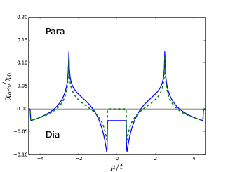
A low-energy approach shows that the scaling of the susceptibility in the gap is different from boron nitride
| (47) |
where the gap is here given by .
V.3.3 Conclusion on gapped systems
The study of gapped systems showed two surprising results. First, a band insulator with a chemical potential lying inside the band gap can have a non-vanishing magnetic susceptibilityFukuyama70 . As the two models we presented above gave a constant diamagnetic susceptibility in the gap, one may argue that it is always diamagnatic and may be understood in a similar way as the diamagnetism of core electrons. However, the calculations of this paper only concern itinerant electrons (core electrons are not included). Furthermore, the study of yet another system, namely a gapped version of the lattice presented in Ref. [Raoux14, ], gives a finite susceptibility in the gap that is continuously tunable from dia- to paramagnetic (without changing the zero-field spectrum).
The second surprising result obtained on gapped system is the behavior near the gap. On the gap edges, the susceptibility is by no mean forced to converge towards the Landau diamagnetic value even if the band spectrum is parabolic. Again, we interpret this result as a proof of interband coupling even for distant bands.
VI Conclusion
The orbital magnetism of isolated atoms was understood long ago. However that of itinerant electrons in crystalline solids has remained in an unsatisfactory state. Roughly speaking, it stayed at the basic understanding that the orbital susceptibility of Bloch electrons is essentially that of free electrons (as understood by LandauLandau30 ) albeit with an effective band mass (expected to take the band structure into account and as understood by PeierlsPeierls33 ): (see e.g. Ref. [Ashcroft, ; Abrikosov72, ]). Actually, the work of Peierls contains more than that but it neglects a crucial ingredient: band coupling or interband effects. Fukuyama made an essential step by providing a compact formula including interband effectsFukuyama71 .
In the present paper, we clarify some aspects of the orbital magnetism of band coupled systems. Using a gauge-independent perturbation theory approach to compute magnetic field derivatives of the grand potential for multi-band tight-binding models, we obtained a new formula – see Eq. (24) – for the orbital susceptibility and recover the known result for the orbital magnetization – see Eq. (20). Then, we obtained a convenient formula for the orbital susceptibility of particle-hole symmetric two-band models – see Eq. (30) – and applied it to several specific models. Equations (24) and (30) are our main results. Here we summarize the lessons that we learned about the orbital magnetism of itinerant electrons in band coupled systems:
-
•
According to “the Ashcroft and Mermin”Ashcroft ; textbooks : “If the electrons move in a periodic potential […], the analysis becomes quite complicated, but again results in a diamagnetic susceptibility of the same order of magnitude as the paramagnetic [Pauli] susceptibility.” We showed that this claim is not true. First, the orbital susceptibility is not always diamagnetic, as understood long ago by VignaleVignale91 and anticipated by PeierlsfootnotePeierls . Actually, for tight-binding models, we proved a sumruleRaoux14 that implies that the orbital susceptibility has to feature both dia- and paramagnetic behaviors as a function of the chemical potential. Secondly, the orbital susceptibility is in general not of the same order of magnitude as the Pauli susceptibility (where is the Bohr magneton). For example, the orbital susceptibility in graphene diverges at half filling as , while the Pauli contribution goes to zero with the DoS .
-
•
The orbital susceptibility obtained from second order perturbation theory is not only given by the zero-field energy spectrum but crucially depends on zero-field eigenstates. Then the LP formula, which only depends on the zero-field energy spectrum, is not exact in the case of several bands. The presence of multiple bands yields interband coupling that drastically affect the susceptibility. Roughly, speaking, these eigenstates effects are thought of as geometrical properties of the Bloch bundle (collectively known as Berry phase effects in solid state physics Xiao10 ) and are a measure of band coupling.
-
•
The Fukuyama formulaFukuyama71 does not generally apply to tight-binding modelsGomez-Santos11 ; Koshino07 . For example, in the case of a single band, it works for the square but not for the triangular lattice tight-binding models (see Appendix C). Actually it fails for non-separable tight-binding models (in Eq. (26), the Fukuyama formula corresponds to ). As such, it does not recover the LP formula in the case of an arbitrary single band model (see the corresponding discussion in Ref. [Fukuyama71, ]). Generally speaking, the Fukuyama formula is not suited for tight-binding models with a finite number of bands, as it was obtained from a different theoretical basis relying on the complete band structure made of an infinite number of bands. It could well be – but we did not prove it – that the Fukuyama formula follows from equation (24) in the limit of an infinite number of bands. We suspect that the non-separability originates from the restriction to a finite number of bands of the complete Hamiltonian.
-
•
The orbital susceptibility is not a Fermi surface property but depends on all the filled bands (see the discussion in Ref. [Haldane04, ]). It contains essential contributions from the bulk of the Fermi sea. This is best illustrated by the susceptibility at the bottom of the conduction band of boron nitride (see Fig. 6): it goes from diamagnetic in the gap to a finite paramagnetic value (roughly given by ) as the chemical potential moves toward the bottom of the conduction band (). This is in complete opposition (both in sign and magnitude) with the naive Landau diamagnetism expectation at a parabolic band edge.
Acknowledgements.
We thank M.O. Goerbig, H. Bouchiat and collaborators for many discussions on orbital magnetism over the years. Note added: During the completion of the present paper, Gao et al. posted a preprint on the arXiv on the geometrical effects in orbital magnetismGao14 . Their result for the orbital susceptibility of boron nitride (see their Fig. 2a) does not agree with ours (see our Fig. 6), which we have confirmed by exact numerical solution (Hofstadter butterfly). For example, it does not satisfy the exact sumrule. In particular, their susceptibility seems to increase near the band edges and to disagree in sign with the Landau-Peierls susceptibility, which should be diamagnetic. In addition, close to the gap (), their susceptibility vanishes, whereas we find a paramagnetic plateau.References
- (1) N.W. Ashcroft & N.D. Mermin, Solid State Physics, Saunders, Philadelphia, pp.664 (1976).
- (2) L.D. Landau, Z. Phys. 64, 629 (1930). See also the Collected papers of L. D. Landau edited by D. ter Haar (Pergamon Press, New York, 1965).
- (3) R. Peierls, Z. Phys. 80, 763 (1933). The English translation can be found in World Scientific Series in 20th Century Physics: Volume 19. Selected Scientific Papers of Sir Rudolf Peierls, (edited by R.H. Dalitz & R. Peierls).
- (4) E.N. Adams, Phys. Rev. 89, 633 (1953).
- (5) J.E. Hebborn & E.H. Sondheimer, J. Phys. Chem. Solids 13, 105 (1960).
- (6) L.M. Roth, J. Phys. Chem. Solids 23, 433 (1962).
- (7) G.H. Wannier, Phys. Rev. 136, A803 (1964).
- (8) P.K. Misra & L.M. Roth, Phys. Rev. 177, 1089 (1969).
- (9) H. Fukuyama, Prog. Theor. Phys. 45, 704 (1971).
- (10) H. Fukuyama & R. Kubo, J. Phys. Soc. Jap. 28, 570 (1970).
- (11) G. Gomez-Santos & T. Stauber, Phys. Rev. Lett. 106, 045504 (2011).
- (12) M. Koshino & T. Ando, Phys. Rev. B 76, 085425 (2007), see in particular the appendix B.
- (13) P.R. Wallace, Phys. Rev. 71, 622 (1947).
- (14) K.S. Novoselov et al., Science 306, 5696 (2004).
- (15) M. Sepioni, R.R. Nair, S. Rablen, J. Narayanan, F. Tuna, R. Winpenny, A.K. Geim & I.V. Grigorieva, Phys. Rev. Lett. 105, 207205 (2010).
- (16) E. G. Nikolaev, A. S. Kotosonov, E. A. Shalashugina, A. M. Troyanovskii & V. I. Tsebro, J. Theor. Exp. Phys. 117, 338 (2013).
- (17) J.W. McClure, Phys. Rev. 104, 606 (1956)
- (18) G. Vignale, Phys. Rev. Lett 67, 358 (1991).
- (19) H. Fukuyama, J. Phys. Soc. Jpn. 76, 043711 (2007).
- (20) A. Raoux, M. Morigi, J.N. Fuchs, F. Piéchon & G. Montambaux, Phys. Rev. Lett. 112, 026402 (2014).
- (21) R. Rammal, J. Phys. (France) 46, 1345 (1985).
- (22) B. Savoie, J. Math. Phys. 53, 073302 (2012).
- (23) K.T. Chen & P.A. Lee, Phys. Rev. B 84, 205137 (2011).
- (24) R. Nourafkan, G. Kotliar & A.M. Tremblay, Phys. Rev. B 90, 125132 (2014).
- (25) S.D. Swiecicki & J.E. Sipe, Phys. Rev. B 90, 125115 (2014).
- (26) T. Thonhauser, Int. J. Mod. Phys B 25, 1429 (2011).
- (27) T. Thonhauser, D. Ceresoli, D. Vanderbilt & R. Resta, Phys. Rev. Lett. 95, 137205 (2005).
- (28) D. Xiao, J. Shi & Q. Niu, Phys. Rev. Lett. 95, 137204 (2005).
- (29) R. Bianco & R. Resta, Phys. Rev. Lett. 110, 087202 (2013).
- (30) D. Xiao, M.C. Chang & Q. Niu, Rev. Mod. Phys. 82, 1959 (2010).
- (31) J.N. Fuchs, F. Piéchon, M.O. Goerbig & G. Montambaux, Eur. Phys. J. B 77, 351 (2010).
- (32) A. Raoux, F. Piéchon, J.N. Fuchs & G. Montambaux (unpublished).
- (33) A.H. Castro Neto, F. Guinea, N.M.R. Peres, K.S. Novoselov & A.K. Geim, Rev. Mod. Phys. 81, 109 (2009).
- (34) F.D.M. Haldane, Phys. Rev. Lett 93, 206602 (2004).
- (35) E. McCann & V. Falko, Phys. Rev. Lett. 96, 086805 (2006); E. McCann, D. Abergel & V. Fal’ko, Eur. Phys. J. Special Topics 148, 91 (2007).
- (36) G. Montambaux, Eur. Phys. J. B 85, 375 (2012).
- (37) S.A. Safran, Phys. Rev. B 30, 421 (1984).
- (38) G. Montambaux, F. Piéchon, J.N. Fuchs & M.O. Goerbig, Eur. Phys. J. B 72, 509 (2009).
- (39) G. Montambaux, F. Piéchon, J.N. Fuchs & M.O. Goerbig, Phys. Rev. B 80, 153412 (2009).
- (40) P. Dietl, F. Piéchon & G. Montambaux, Phys. Rev. Lett. 100, 236405 (2008).
- (41) S. Banerjee & W.E. Pickett, Phys. Rev. B 86, 075124 (2012).
- (42) G.W. Semenoff, Phys. Rev. Lett. 53, 26 (1984).
- (43) M. Nakamura, Phys. Rev. B 76, 113301 (2007).
- (44) M. Koshino & T. Ando, Phys. Rev. B 81, 195431 (2010).
- (45) A. Abrikosov, Introduction to the theory of normal metals, §10.3 (Academic Press, 1972).
- (46) Other solid state physics textbooks either do not dare writing anything about orbital magnetism of conduction electrons (see, e.g., C. Kittel, Introduction to solid state physics, (8th edition, Wiley, 2005)) or are restricted to the Landau result for free electrons (see, e.g., M.P. Marder, Condensed matter physics, 2nd edition, (Wiley, 2010) or C. Kittel, Quantum theory of solids, (Wiley, 1987)).
- (47) Eventhough his paper is entitled “On the diamagnetism of conduction electrons”, Peierls understood that the orbital susceptibility may change sign to become paramagnetic (see page 117 of the English translation of Ref. Peierls33, ).
- (48) Y. Gao, S.A. Yang & Q. Niu, arxiv:1411.0324 .
- (49) P. Skudlarski & G. Vignale, Phys. Rev. B 43, 5764 (1991).
Appendix A Orbital Magnetization
The starting point to derive Eq. (20), is to calculate the trace of Eq. (18):
| (48) |
The Green’s function can be written in terms of the Bloch state and the energy dispersion of the band:
| (49) |
One gets
| (50) |
where , is the cell-periodic part of the Bloch state and is a projector. Knowing that
| (51) |
Eq. (50) can be transformed using the definitions in Eqs. (21, 22) (and a change of indices for the last term of Eq. (51)):
| (52) |
Computing the integral over the energy with the formula
| (53) |
allows us to finish the calculation and to recover Eq. (20).
Appendix B Partial Integration for Tr
Starting from Eq. (23), and using the identity , the trace of reads:
| (54) |
with
| (55) |
Using the identity and the cyclicity of the trace , one verifies
| (56) |
where
| (57) |
Using again the cyclicity of the trace, one can further establish the identity:
| (58) |
where . Using Eqs. (54, 56, 58), one finally obtains the following three equivalent writtings:
| (59) |
where the second line corresponds to Eq. (23) that allows to obtain susceptibility formula Eq. (24), whereas the third line allows to recover susceptibility formula Eq. (26) first derived in Gomez-Santos11 . Note that represents the second order correction to the integrated DoS. Since the total number of states is magnetic field independent, necessarily vanishes outside the zero-field energy bandwidth.
Appendix C Landau-Peierls formula for single-band models
For a single band tight-binding model, the LP susceptibility
| (60) |
is exact (it is easily derived from Eq. (24)). The magnetic response of the square and triangular lattices are here investigated in order to illustrate the (not so well-known) physics contained in this formula.
Note that, apart from the derivative of the Fermi function, the integrand of Eq. (60) can be understood as the determinant of the Hessian matrix of the spectrum . The susceptibility is thus governed by an intrinsic geometrical quantity of the spectrum: the Hessian , which is almost the Gaussian curvature of the band spectrum. When the spectrum can be approximate to a quadratic dispersion, it reads with and the two effective masses of the spectrum. Thus, for a parabolic spectrum at zero temperature
| (61) |
with the DoS at the Fermi energy . From Eq. (61), we deduce that the LP susceptibility diverges when the DoS does; and can change sign at a saddle point, i.e. when and have different signsVignale91 . The physical picture behind such a behavior was provided by VignaleVignale91 : it is that of a counter-circulating orbit around the saddle point. The latter is made of pieces of four regular cyclotron orbits connected by quantum mechanical tunneling events (known as magnetic breakdown in this context).
C.1 Square lattice
The dispersion relation for the square lattice (with and )
| (62) |
is separable. We find a simple susceptibility (with ):
| (63) |
where is the Legendre function of the second kind. This compact formula is consistent with another one proposed in Ref. [Skudlarski91, ]. This is plotted in Fig. (8).
Some features of this figure are worth commenting on:
-
1.
The susceptibility can be either positive or negative. The situation is different from free particles where the susceptibility is always negative (Landau diamagnetism).
-
2.
The susceptibility verifies the sumrule: and thus it has both dia- or para-magnetic behavior depending on .
-
3.
In the vicinity of the band edges (band bottom and band top), the susceptibility tends to a diamagnetic value, which is exactly the Landau susceptibility with an effective band mass . In the limit of low/high filling, we recover free electrons/holes with an effective mass.
-
4.
At half filling (vanishing chemical potential), the susceptibility is paramagnetic and diverges logarithmically. This is a consequence of the van Hove singularity in the DoS. The latter is related to saddle points in the spectrum, at which the effective masses and are of different signs, leading to orbital paramagnetism.
C.2 Triangular lattice
The nearest-neighbor tight-binding model on the triangular lattice is quite interesting as it has a dispersion relation which is not separable. This will allow us to compare several predictions for the orbital susceptibility. The dispersion relation is (with and )
| (64) |
Since there is only one band, the exact orbital susceptibility is given by the LP formula (60) and satisfies the sumrule. Here, in contrast to the square lattice, . The result is plotted in Fig. 9.
Other single-band formulas, which exist in the literature, disagree with the above exact result. For example, application of the Fukuyama formula gives the following susceptibilityFukuyama71 :
| (65) |
It is obtained from Eq. (26) by keeping only the first term (with four Green’s functions ) and restricting to a single band model. On the second expression above (involving ), it is easy to check that it satisfies the sumrule. It is also plotted in Fig. 9.
Another formula was proposed by Hebborn and Sondheimer (HS), which in the single band case reduces toFukuyama71
| (66) |
It is almost identical to the expression for except that it involves the Hessian . However, it does not satisfy the sumrule. It is plotted in Fig. 9 as well.
C.3 Conclusion on the orbital susceptibility in the case of a single band
On the one-hand, the tight-binding model on the square lattice is separable (). In this case, the LP, the Fukuyama and the HS susceptibilities all agree. On the other hand, the tight-binding model on the triangular lattice is not separable () and allows one to discriminate between the different predictions. The LP susceptibility is exact in the case of a single band (whether separable or not). In addition, it does satisfy the sumrule. The Fukuyama formula also satisfies the sumrule, but it strongly disagrees with the exact result. For example, it predicts a strange diamagnetic peak at the van Hove singularity (when a paramagnetic peak is generally expectedVignale91 ). The HS susceptibility is closer to the exact result but is also wrong and does not satisfy the sumrule.
Appendix D 2-band derivation
D.1 Definitions
The aim of this section is to derive a computable two-band formula for the susceptibility of particle-hole symmetric systems. In order to use Eq. (24), we first need to compute the successive derivatives of (where is here a shorthand notation for ) (as described in Sec. V). They read:
| (67) | ||||
| (68) | ||||
| (69) |
with .
The effect of a projector onto the derivatives of is given by:
| (70) | ||||
| (71) | ||||
| (72) | ||||
| (73) |
Finally, the following identity will reveal to be useful in the following:
| (74) |
D.2 Two-Green’s functions term
is first investigated. On the eigenprojectors basis,
| (75) |
with
| (76) |
After some algebra, one gets:
| (77) | |||
| (78) |
such that:
| (79) |
The second term of Eq. (79) can be splited in two such that
| (80) | ||||
| (81) |
where
| (82) | ||||
| (83) |
D.3 Four-Green’s functions term
D.4 Results
The product of Green’s functions has to be decomposed to compute the integral over the energy:
| (97) | ||||
| (98) | ||||
| (99) |
and using
| (100) |
where is the derivative of , the integral over can be performed
| (101) | |||
| (102) |
with a shorthand notation for and , are first and second derivatives of .
Appendix E Low-energy approach
The idea behind the low-energy approach is to compute the susceptibility using formula (24), but with a simplified (linear or quadratic) Hamiltonian obtained in the vicinity of an energy of interest (for example a band touching point). The graphene Hamiltonian is approximated by the linearised massless Dirac Hamiltonian (for a single valley). This approximation is expected to be true for vanishing chemical potential only. Thus, with the linear approximation of near a Dirac point . Writing , the approximate Hamiltonian is .
The second term of Eq. (24) vanishes because of the linearity of the spectrum. The approximate Green’s function yields
| (103) |
such that
| (104) |
To compute the double integral on and , polar coordinates and () are more adequate:
| (105) |
With a partial fraction decomposition of with , the integral over can be performed:
| (106) |
Finally, the integral over the energy is computed using Eq. (53):
| (107) |
taking into account the two valleys. This is the result of Eq. (40). Note, however, that this approach does not capture the paramagnetic plateau . Indeed, the correct result in the vicinity of is . This shows that a low-energy approach, that includes band coupling, i.e. the spinor structure of the massless Dirac wavefunction, in the vicinity of does not fully recover the correct orbital susceptibility. This proves that the latter is not a Fermi surface property only but also depends on all the filled bands.