Centre for Fusion, Space, and Astrophysics, Department of Physics, University of Warwick, Coventry CV4 7AL, UK
Tel.: +44-2476-574211
Fax: +44-2476-150897
22email: a-m.broomhall@warwick.ac.uk 33institutetext: P. Chatterjee 44institutetext: High Altitude Observatory, National Center for Atmospheric Research, PO Box 3000, Boulder CO 80307, USA
44email: mppiyali@ucar.edu 55institutetext: R. Howe 66institutetext: School of Physics and Astronomy, University of Birmingham, Edgbaston, Birmingham, B15 2TT, UK
66email: rhowe@noao.edu 77institutetext: A.A. Norton 88institutetext: HEPL, Solar Physics, Stanford University, CA 94305 USA
88email: aanorton@stanford.edu 99institutetext: M.J. Thompson 1010institutetext: High Altitude Observatory, National Center for Atmospheric Research, PO Box 3000, Boulder CO 80307, USA
1010email: mjt@ucar.edu
The Sun’s interior structure and dynamics, and the solar cycle
Abstract
The Sun’s internal structure and dynamics can be studied with helioseismology, which uses the Sun’s natural acoustic oscillations to build up a profile of the solar interior. We discuss how solar acoustic oscillations are affected by the Sun’s magnetic field. Careful observations of these effects can be inverted to determine the variations in the structure and dynamics of the Sun’s interior as the solar cycle progresses. Observed variations in the structure and dynamics can then be used to inform models of the solar dynamo, which are crucial to our understanding of how the Sun’s magnetic field is generated and maintained.
Keywords:
Sun: activity Sun: helioseismology Sun: interior Sun: magnetic fields Sun: oscillations1 Introduction to helioseismology
Helioseismology is the study of the solar interior using observations of waves that propagate within the Sun. The Sun’s natural acoustic resonant oscillations are known as solar p modes. The p stands for pressure as the main restoring force is a pressure differential. At any one time thousands of acoustic oscillations are traveling throughout the solar interior. Each individual solar p mode is trapped in a specific region of the solar interior, known as a cavity, and its frequency is sensitive to properties, such as temperature and mean molecular weight, of the solar material in the cavity. The sound waves can be considered as damped harmonic oscillators as they are stochastically excited and intrinsically damped by turbulent convection in the outer approximately 30 per cent by radius of the solar interior. The strongest p-mode oscillations have a periodicity of approximately 5 minutes. The solar oscillations can be observed in two ways: by line-of-sight Doppler velocity measurements over the visible disk; or by measuring the variations in the continuum intensity of radiation, which are caused by the compression of the radiating gas by the waves.
The horizontal structure of p modes can be modeled as spherical harmonics and so can be described by three main components: Harmonic degree, , which indicates the number of node lines on the surface; azimuthal degree, , which describes the number of planes slicing through the equator and takes values between ; and radial degree, , which gives the number of radial nodes in the solar interior. If the Sun was completely spherically symmetric the frequencies of the oscillations would be degenerate in . However, asphericities in the solar interior, such as rotation, temperature variations and the presence of magnetic fields, lift the degeneracy and measurements of the differences in the frequencies of the components allow inferences to be made concerning the effects responsible for the asphericities.
The frequency of a mode, , can be expressed in terms of the central frequency, , and a polynomial expansion of splitting (or ) coefficients, :
| (1) |
where are the Ritzwoller-Lavely formulation of the Clebsch-Gordon expansion (Ritzwoller and Lavely, 1991) and are given by
| (2) |
Here, are the Clebsch-Gordon coefficients. The odd-order coefficients express the difference in mode frequency caused by the modes’ interaction with the rotation profile of the solar interior. The even-order coefficients are sensitive to all other departures from spherical symmetry. These could include local variations in the sound speed or cavity size (Balmforth et al., 1996), temperature variations (Kuhn, 1988), second order rotation effects from the differential rotation (Dziembowski and Goode, 1992), and the presence of magnetic fields (Gough and Thompson, 1988b). Isolating the contributions of all these effects to the even-order coefficients is extremely difficult.
As sound waves travel from their excitation point near the surface into the solar interior they are refracted because of increasing pressure, and therefore sound speed (since , where is the first adiabatic exponent). Assuming the direction of travel is not radial the waves follow a curved trajectory which takes them back to the surface where they are reflected by the sharp drop in density. By the time the waves reach the surface they are approximately traveling in a radial direction and so the depth at which the near-surface reflection of the waves occurs depends only on the wave frequency. The p modes are set up by a superposition of such waves, and so the location of the upper edge of the acoustic cavity of the modes – the upper turning point – likewise depends only on frequency, with the upper turning point of low-frequency modes being deeper in the solar interior than the upper turning point of high-frequency modes. The radius of the lower turning point depends on the angle of trajectory and therefore , with low- modes turning deeper within the solar interior than high- modes.
Helioseismology can be split into two categories: global and local. Global helioseismology studies the natural resonant acoustic oscillations of the solar interior that are able to form standing waves in the entire Sun, as opposed to local helioseismology, which studies propagating waves in part of the Sun. We now give a brief introduction to each category.
1.1 Global helioseismology
Global helioseismology can itself be split into two sub-categories: Sun-as-a-star (unresolved) observations; and resolved observations. Sun-as-a-star observations are only sensitive to the lowest harmonic degrees (, and occasionally and 5). These modes are the truly global modes of the Sun as they travel right to the energy-generating core. However, by making resolved observations of the solar surface spatial filters can be applied that allow measurements of modes with degrees into the 100s or even 1000s.
The Birmingham Solar Oscillations Network (BiSON, Elsworth et al., 1995; Chaplin et al., 1996) has been making Sun-as-a-star line-of-sight velocity observations for over 30 years, covering cycles 21 (although with limited coverage), 22, 23, and 24. BiSON is an autonomous network of 6 ground-based observatories strategically positioned around the world so as to allow observations of the Sun to be made 24 hr a day. This is important as gaps in the time domain contaminate frequency spectra, making it more difficult to accurately obtain the parameters that describe the modes, such as their frequencies. One can also make continuous observations of the Sun from space and this is the approach taken by the SOlar and Heliospheric Observatory (SOHO) spacecraft, which was launched in 1995. Sun-as-a-star observing programs onboard SOHO include the Global Oscillations at Low Frequencies (GOLF; Gabriel et al., 1995) instrument, which also measures line-of-sight velocity, and the Variability of solar IRrandiance and Gravity Oscillations (VIRGO; Fröhlich et al., 1995), which measures the changes in intensity of the Sun.
VIRGO is also capable of making resolved observations of the Sun, as was the Michelson Doppler Imager (MDI; Scherrer et al., 1995), also onboard SOHO. Global Oscillations Network Group (GONG) is a ground-based network of 6 sites (Harvey et al., 1996), which has been making resolved observations of the Sun since 1995. More recently, the Helioseismic and Magnetic Imager (HMI; Schou et al., 2012) and the Atmospheric Imaging Assembly (AIA; Lemen et al., 2012) onboard the Solar Dynamics Observatory (SDO) have been used for helioseismic studies (Howe et al., 2011a, b). SDO was only launched in 2010 and so these instruments cannot be used to study previous solar cycles. They are, however, likely to play an important role in helioseismic studies of cycle 24, and possibly beyond.
1.2 Local helioseismology
Since the advent of helioseismic observations at high spatial resolution, a number of different data analysis techniques known collectively as “local helioseismology” have been developed. They do not rely on the global resonant-mode nature of the observed oscillations: rather, the observations of wave motions are interpreted in terms of their local properties. Three methods in particular are widely used. Ring analysis (or ring-diagram analysis) works within a freqeuncy-wavenumber framework for analysing the oscillations, albeit on localized patches of the solar surface, and may therefore be considered the local-helioseismic analogue of global-mode helioseismology. Time-distance helioseismology (or helioseismic tomography), and the closely related method of acoustic holography, work rather in the framework of interpreting the effect of heterogeneities and flows on propagating waves in terms of travel-time shifts or equivalently phase shifts. These two basically distinct approaches will be described briefly below.
In ring analysis (Hill, 1989), measurements of wave properties are made in localized regions (“tiles”) on the surface of the Sun. The observable - typically the Doppler velocity - over the pixels within the region are Fourier transformed in the two spatial horizontal directions and in time to give wave power as a function of spatial wavenumbers , and frequency. In cuts through the 3-D power spectrum at fixed frequency, the power is found to lie in rings corresponding to the different radial orders of the modes: hence the name “ring analysis”. In the absence of flows or any horizontal inhomogeneities, the dispersion relation of the waves is of the form , where is the magnitude of the horizontal wavenumber vector. In other words, the frequencies do not depend on the direction of the horizontal wavenumber, only on its magnitude: thus, the rings of power are circular and centered on . Large-scale flows and magnetic fields, which can change the dispersion relation depending on the direction of propagation of the waves, shift and distort the rings. Further, local changes in the effective isotropic wave speed (such as could be caused by thermal anisotropies) change the frequency at fixed wavenumber or equivalently change the radius of the rings at fixed frequency. These various perturbations to the rings, measured at different frequencies and for different values, permit the possibility of performing a one-dimensional inversion in depth to infer the large-scale flow, wave speed, etc., below each tile (Haber et al., 2002; Bogart et al., 2008; González Hernández et al., 2010). By combining inversion results under different tiles, a three-dimensional subsurface map can be built up. Recently, fully 3-D inversion methods have been developed and implemented that simultaneously invert the data from many different tiles to obtain 3-D maps of subsurface flows directly (Featherstone et al., 2011).
In time-distance helioseismology, travel times of waves that propagate beneath the surface between pairs of surface points are estimated by cross-correlating the observed oscillations between surface points. The cross-correlation function derived by cross-correlating the oscillations at two surface points A and B, say, exhibits a number of “wave packets”. In a ray-theoretic interpretation, these packets correspond to waves that travel between A and B along different ray paths, either traveling directly without intermediate surface bounces, or bouncing at the surface one or more times before arriving at the point of observation. In practice, it can be necessary to average the cross-correlations between many similarly separated pairs of points before the wave packets are clearly visible . Partly for this reason, the observations are typically filtered in some way before the cross-correlations are made. The most common filters are a phase-speed filter or a filter that aims to isolate oscillations corresponding to a particular radial order . Also, usually it is only the first-arrival wave packet – corresponding to propagation between A and B with no intermediate surface bounces – that is used in the subsequent analysis. Travel times are estimated by measuring the location of the wave packet, and a number of different methods are used to do that. Flows, magnetic fields and inhomogeneities experienced by the waves during their propagation from A to B shift the location of the wave packet (and this in turn is measured as a travel-time shift) as well as potentially modifying the width and amplitude of the wave packet. Also, flows can cause a difference in travel time depending on whether the waves are traveling from A to B or from B to A. By measuring travel times between many different pairs of surface points, 3-D subsurface maps of flows and wave-speed inhomogeneities can be made using inverse techniques (Zhao and Kosovichev, 2004).
For further discussion of the signatures of flows on the ring analysis and time-distance helioseismology measurements, see Section 5.1. For now, however, we return to concentrate on the global modes.
2 An introduction to global helioseismology and the solar cycle
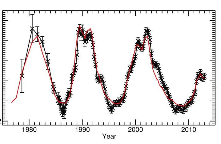
It has been known since the mid 1980s that p-mode frequencies vary throughout the solar cycle with the frequencies being at their largest when the solar activity is at its maximum (e.g. Woodard and Noyes, 1985; Pallé et al., 1989; Elsworth et al., 1990; Libbrecht and Woodard, 1990; Chaplin et al., 2007; Jiménez-Reyes et al., 2007).111Please note here that the references listed are not exhaustive, instead we have tried to include useful ones whose reference lists themselves are informative. For a low- mode at about the change in frequency between solar maximum and minimum is about . By examining the changes in the observed p-mode frequencies throughout the solar cycle we can learn about solar-cycle-related processes that occur beneath the Sun’s surface. The 11 year cycle is seen clearly in Fig. 1, which shows the mean frequency shifts of the p modes observed by BiSON and the 10.7cm flux222http://www.ngdc.noaa.gov/stp/space-weather/solar-data/solar-features/solar-radio/noontime-flux/penticton/ for comparison (also see Broomhall et al., 2009; Salabert et al., 2009; Fletcher et al., 2010).
What causes the observed frequency shifts? The magnetic fields can affect the modes in two ways: directly and indirectly. The direct effect occurs because the Lorentz force provides an additional restoring force resulting in an increase of frequency, and the appearance of new modes. Magnetic fields can influence the oscillations indirectly by affecting the physical properties of the cavities in which the modes are trapped and, as a result, the propagation of the acoustic waves within them. For example, changes in the thermal structure can affect both the propagation speed and the location of the upper turning point. Indirect effects can both increase or decrease the frequencies of p modes.
To date the relative contributions from the direct and indirect effects remain uncertain. Dziembowski and Goode (2005) suggest that the magnetic fields are too weak in the near-surface layers for the direct effect to contribute significantly to the observed frequency shifts and that the indirect effects dominate the perturbations. However, Dziembowski and Goode also suggest that the direct effect may be more important for low-frequency modes deeper within the solar interior where the magnetic field is strong enough to produce a noticeable shift in frequency. These results are still controversial and appear to disagree with the results of Roberts and Campbell (1986), who found that field strengths of the order of 500 kG would be required at the base of the convection zone to explain the shift. Foullon and Roberts (2005) investigated the effect of a magnetic field at the base of the convection zone and a more shallow magnetic field, at a depth of 50 Mm, but found their direct influence on the frequencies of p modes was consistently smaller than the change in frequency that is observed. Changes in both the chromospheric magnetic field strength and temperature can explain the observed downturn in the magnitude of the frequency shifts at high frequencies (Jain and Roberts, 1993). However, as we now describe, it is not only the mode frequencies that vary throughout the solar cycle.
2.1 Solar cycle variations in mode powers and lifetimes
Solar p modes are excited and damped by turbulent convection beneath the solar surface. The process of excitation and damping varies throughout the solar cycle and these variations are observed as changes in the heights and widths of the mode profiles in a frequency-power spectrum. For typical low- modes, as the surface activity increases the mode frequencies and widths increase but the mode heights decrease. An increase in the linewidths implies that the modes experience more damping at times of high activity and so the lifetimes decrease.
Numerous authors have observed that lifetimes decrease with solar activity and those observations have been made using data from different instrumental regimes and for a range of (e.g. Jefferies et al., 1990; Pallé et al., 1990; Chaplin et al., 2000; Komm et al., 2000; Appourchaux, 2001; Toutain and Kosovichev, 2001; Jiménez et al., 2002; Howe et al., 2003; Jiménez-Reyes et al., 2004b; Salabert and Jiménez-Reyes, 2006; Burtseva et al., 2009; Simoniello et al., 2010). The size of the variation appears to be dependent on with lower- modes showing a larger percentage change than high- modes (e.g. Burtseva et al., 2009, and references therein). Burtseva et al. (2009) looked at the lifetimes of modes with and found that in active regions the lifetimes decrease as activity increases by about 13% between minimum and maximum. In quiet regions the lifetimes still decrease with solar activity but to a lesser extent (the lifetimes at solar maximum are about 8% of the lifetimes at solar minimum). This implies that the change to the damping is not just associated with the active regions that appear on the surface. In general p-mode linewidths increase with frequency, except for a plateau region at around . Komm et al. (2000) found that the linewidths of modes in the plateau region were most sensitive to the level of solar activity.
Mode powers have been observed to decrease with increasing solar activity (e.g. Pallé et al., 1990; Anguera Gubau et al., 1992; Elsworth et al., 1993). The decrease in mode power is of the order of 20% and has been now been observed by many authors (e.g. Chaplin et al., 2000; Komm et al., 2000; Jiménez-Reyes et al., 2001; Appourchaux, 2001; Toutain and Kosovichev, 2001; Jiménez et al., 2002; Jiménez-Reyes et al., 2004b; Simoniello et al., 2009). The total energy of the mode, , can be determined by multiplying the total power of the mode by the mode mass (as defined by Christensen-Dalsgaard and Berthomieu, 1991). The mode energy shows a similar decrease to the mode power, with a maximum to minimum variation of approximately 12% (Jiménez et al., 2002).
The energy supply rate is determined by multiplying the mode energy by the mode width (e.g. Chaplin et al., 2000). Numerous studies have shown that while the mode energy decreases with activity the energy supply rate shows no solar cycle variation (e.g. Chaplin et al., 2000; Komm et al., 2000; Appourchaux, 2001; Toutain and Kosovichev, 2001; Jiménez et al., 2002; Howe et al., 2003; Jiménez-Reyes et al., 2004b; Salabert and Jiménez-Reyes, 2006). Therefore, the observed variations in mode energy and mode power probably arise from an increase in damping only. As the energy of the modes decreases between solar minimum and solar maximum this implies that some energy has gone missing.
One potential source of damping is magnetic activity on the solar surface. Active regions are known to suppress the power of p modes, and effect lifetimes, and energy supply rates (e.g. Woods and Cram, 1981; Lites et al., 1982; Brown et al., 1992; Rajaguru et al., 2001; Komm et al., 2002; Howe et al., 2004a). However, the associated mechanisms are not yet fully understood. One explanation is that strong-field magnetic regions, such as sunspots, are effective absorbers of p-mode power (e.g. Haber et al., 1999; Jain and Haber, 2002). Komm et al. (2000) suggested that the energy could be in flux tubes, whose numbers increase with solar activity, and the energy could excite oscillations in magnetic elements. Another suggestion is that the efficiency of mode excitation is reduced in magnetic areas (e.g. Goldreich and Kumar, 1988; Cally, 1995; Jain et al., 1996). Other possible explanations as to why p-mode excitation is suppressed in sunspots include a different height of spectral line formation due to the Wilson depression or a modification of p-mode eigenfunctions by the magnetic field (Burtseva et al., 2009, and references therein).
Another possibility that could alter p-mode damping is variations in the convective properties near the solar surface, which are most likely to arise from the influence of magnetic structures (Houdek et al., 2001). Houdek et al. theorized that changes of parameters in the convection zone would affect linewidth shapes mainly in the plateau region of a frequency spectrum, as is observed. This, therefore, implies that during times of high-magnetic activity the convection zone is affected sufficiently to produce a measurable change in p-mode linewidths. Several authors have observed that the horizontal size of solar granules decreases from solar minimum to solar maximum (e.g. Macris et al., 1984; Muller, 1988; Berrilli et al., 1999; Muller et al., 2007). Muller (1988) found that the horizontal granule size decreased by approximately 5% from solar minimum to solar maximum. According to Houdek et al. (2001) this should result in an increase in damping rates of about 20%, which is in reasonable agreement with the observed change in damping rates in BiSON data of approximately %.
We now return to look in more detail at the changes in frequencies of the p modes with solar cycle.
3 Dependence of solar cycle frequency shifts on and frequency
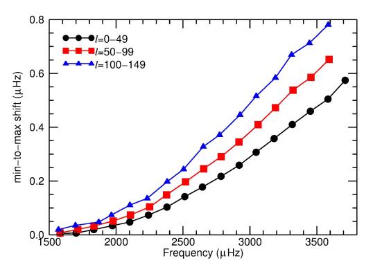
Solar cycle frequency shifts, , have well-known dependencies on both angular degree, , and frequency, , as demonstrated in Fig. 2 (also see e.g. Libbrecht and Woodard, 1990; Elsworth et al., 1994; Chaplin et al., 1998; Howe et al., 1999; Chaplin et al., 2001; Jiménez-Reyes et al., 2001). We now look in more detail at these dependencies and discuss what they tell us about the origin of the perturbation. We note here that the frequency shifts plotted in Fig. 2 were determined for the central frequency of the mode i.e. the frequency. In section 3.3 we discuss the latitudinal dependence of the shifts and there we consider modes with different .
3.1 Dependence of solar cycle frequency shifts on mode inertia
The main -dependence in is associated with mode inertia. The normalized mode inertia is defined by Christensen-Dalsgaard and Berthomieu (1991) as
| (3) |
where is the displacement associated with a mode, suitably normalized at the photosphere, is the volume of the Sun, and is the mass of the Sun. is the ‘mass’ associated with a mode. The physical interpretation of the mode inertia is some measure of the interior mass affected by any given mode. At fixed frequency a decrease in results in an increase in and therefore in . In other words as decreases a greater volume of the interior is associated with the motions generated by the mode. Therefore the high- modes are more sensitive to a perturbation and so vary more throughout the solar cycle than low- modes.
The inertia ratio, , is defined by Christensen-Dalsgaard and Berthomieu (1991) as:
| (4) |
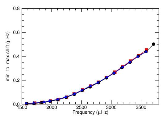
is the inertia an modes would have at a frequency . Multiplying the frequency shifts by removes the dependence of the frequency shifts at fixed frequency, as can be seen in Fig. 2. This makes the dependence a function of frequency alone. Collapsing the dependence in this manner allows the frequency shifts of a wide range of to be combined, thereby reducing any uncertainties associated with the shifts and allowing tighter constraints to be placed on the frequency dependence.
3.2 Dependence of solar cycle frequency shifts on mode frequency
The frequency dependence of the frequency shifts, which can be seen in the right-hand panel of Fig. 2, is a telltale indicator that the observed 11-year signal must be the result of changes in acoustic properties in the few hundred kilometres just beneath the visible surface of the Sun, a region to which the higher-frequency modes are much more sensitive than their lower-frequency counterparts because of differences in the upper boundaries of the cavities in which the modes are trapped (Libbrecht and Woodard, 1990; Christensen-Dalsgaard and Berthomieu, 1991). We now go into more detail.
As mentioned earlier, for a given the upper turning point of low-frequency modes is deeper than the upper turning point of high-frequency modes. At a fixed frequency lower- modes penetrate more deeply into the solar interior than higher- modes. Therefore, higher-frequency modes, and to a lesser extent higher- modes, are more sensitive to surface perturbations.
Libbrecht and Woodard (1990) discuss the origin of the perturbation. If the perturbations were to extend over a significant fraction of the solar interior, asymptotic theory implies that the fractional mode frequency shift would depend mainly on , which is not what we observe. This implies that the relevant structural changes occur mainly in a thin layer. Thompson (1988) found that the effect of perturbing a thin layer in the propagating regions of modes, such as the layer where the second-ionization of helium occurs, is an oscillatory frequency dependence in . Such a frequency dependence is also not observed, implying that the dominant frequency dependence is not the direct result of, for example, changes in the magnetic field at the base of the convection zone. If the perturbation was confined to the centre of the Sun the size of the frequency shift would increase with decreasing as low- modes penetrate deeper into the solar interior than high- modes. In fact, increases with increasing .
We can think of the frequency dependence as a power law where . A perturbation from a layer strictly confined to the photosphere (but extending over less than one pressure scale height) is expected to result in an relationship (Cox, 1980; Gough, 1990; Libbrecht and Woodard, 1990; Goldreich et al., 1991). If instead the perturbation extends beneath the surface, the frequency dependence will be weaker and will get smaller (Gough, 1990). Chaplin et al. (2001) determined that , which implies that the significant contribution comes from a perturbation close to the surface, in the sub-photospheric layers. Rabello-Soares et al. (2008) observed that is smaller for the lower-frequency modes, which suggests that the perturbation extends to greater depths the lower in frequency one goes. This is consistent with the results of Dziembowski and Goode (2005) (see Section 2).
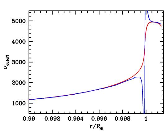
In summary, the oscillations are responding to changes in the strength of the solar magnetic activity near the Sun’s surface. As modes below approximately experience almost no solar cycle frequency shift it is reasonable to conclude that the origin of the perturbation is concentrated in a region above the upper turning points of these modes. Fig. 3 shows that the upper turning point of a mode with a frequency of is about (approximately 3 Mm) below the surface. Note that the upper turning point predicted by a model is strongly dependent on the properties of the model at the top of the convection zone.
Above the relationship between frequency shift and activity changes, as the magnitude of the solar cycle frequency shift decreases and oscillates (e.g. Libbrecht and Woodard, 1990; Goldreich et al., 1991; Jain and Roberts, 1996). Furthermore, above it appears that modes experience a decrease in frequency as activity increases (Ronan et al., 1994; Chaplin et al., 1998).
As we have seen the frequency dependence of the frequency shifts implies that the shifts can be associated with a near-surface perturbation. Therefore, we now move on to directly compare the change in mode frequency with the magnetic field that is observed at the solar surface (and beyond into the solar atmosphere).
3.3 Comparison between frequency shifts and the surface magnetic field
Numerous comparisons have been made between the p-mode frequency shifts and various proxies of the Sun’s surface magnetic field (e.g. Jimenez-Reyes et al., 1998; Antia et al., 2001; Tripathy et al., 2001; Howe et al., 2002; Chaplin et al., 2004b, 2007; Jain et al., 2009, 2012), including the 10.7 cm and the International Sunspot Number333http://www.ngdc.noaa.gov/stp/space-weather/solar-data/solar-indices/sunspot-numbers/international/ (ISN). Chaplin et al. (2007) compared six different proxies with the low- mode frequency shifts and demonstrated that better correlations are observed with proxies that measure both the strong and the weak components of the Sun’s magnetic field, such as the Mg II H and K core-to-wing data, the 10.7 cm radio flux, and the He I equivalent width data (as opposed the the ISN and the Kitt Peak Magnetic Index, which mainly sample the strong magnetic flux). The weak-component of the solar magnetic flux is distributed over a wider range of latitudes than the strong component and so a possible explanation of these results is in terms of the latitudinal distribution of the modes used in this study (i.e. low- modes).
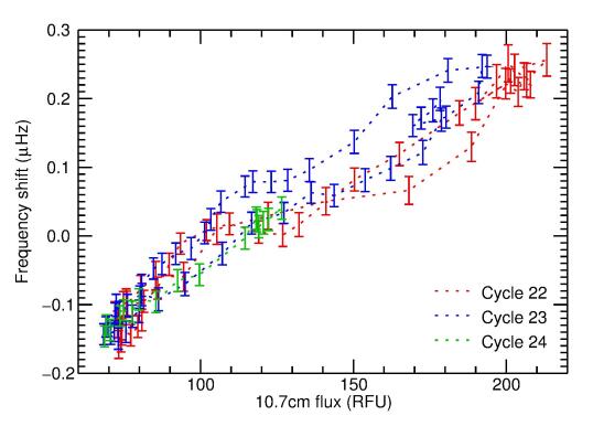
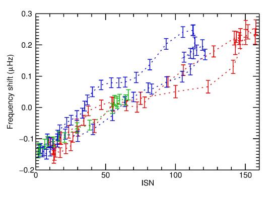
Fig. 4 shows a comparison between two proxies of the Sun’s magnetic field and low- frequency shifts. Although the agreement is approximately linear the well-known hysteresis is clearly visible, particularly in the case of the sunspot number. This can be explained in terms of the variation in the latitudinal distribution of the surface magnetic field throughout the solar cycle (Moreno-Insertis and Solanki, 2000): The different modes have different latitudinal dependencies, as described by the appropriate spherical harmonics (see Section 1), and so the relative influence of the surface magnetic flux on the modes changes throughout the solar cycle as the strong surface magnetic field migrates towards the equator.
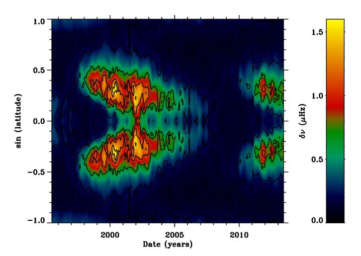
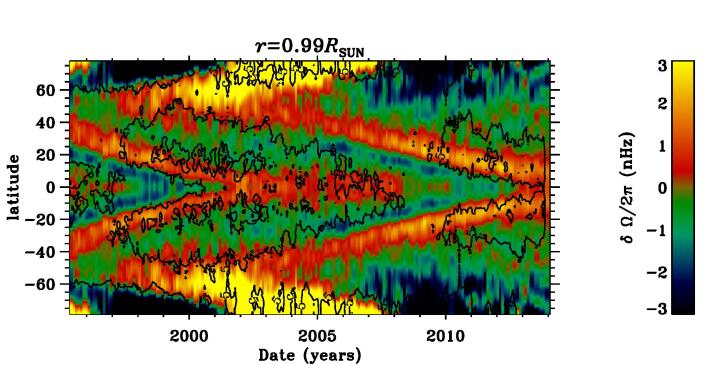
As mentioned in Section 1 the even splitting coefficients can provide information about departures from spherical symmetry, such as those produced by the presence of a magnetic field. Although the correlation between the even coefficients and global measures of the Sun’s magnetic field is good, it is not linear. However, the even splitting coefficients are linearly correlated with the corresponding Legendre polynomial decomposition of the surface (e.g. Howe et al., 1999, 2002; Chaplin et al., 2003, 2004a, 2004b; Jiménez-Reyes et al., 2004a) indicating that the size of the observed frequency shift experienced by a particular mode is dependent on the latitudinal distribution of the surface magnetic flux. Furthermore, Howe et al. (2002) showed that it is possible to use latitudinal inversion techniques to localize the frequency shifts in latitude and, in fact, reconstruct the evolution of the surface magnetic field. An up-to-date version of these inversions can be seen in Fig. 5, which clearly resembles the familiar butterfly diagrams usually associated with the surface magnetic field.
4 Evidence for structural changes due to magnetic fields deeper in the interior
All that has been discussed above concerns the near-surface magnetic field. However, one of the main advantages of helioseismology is that it allows the deeper interior to be studied. Therefore we now move on to discuss attempts to detect evidence of the solar magnetic field deeper in the solar interior. However, this is understandably hard. The plasma- in the deep interior is significantly greater than unity. Furthermore, the sound speed in the interior increases substantially with depth, meaning the modes spend significantly longer in the near-surface regions than in the deep interior. All this means that the influence of a deep-seated magnetic field on the properties of the oscillations will be limited. However, the rewards for finding evidence of deep-seated magnetic fields are great. For example, many believe the solar dynamo is generated in the tachocline at the base of the convection zone (see Charbonneau, 2010, for a recent review).
Numerous authors have looked but were unable to find helioseismic evidence for magnetic fields deeper in the solar interior (e.g. Gough and Thompson, 1988a; Basu and Antia, 2000; Basu and Schou, 2000; Antia et al., 2001; Basu and Antia, 2001; Basu, 2002; Basu and Antia, 2003; Eff-Darwich et al., 2002; Basu et al., 2003). They therefore resorted to putting limits on parameters at the base of the convection zone, such as a maximum change in field strength between solar minimum and maximum of 300 kG (Basu, 1997; Antia et al., 2000) or a change in sound speed of (Eff-Darwich et al., 2002).
Chou and Serebryanskiy (2005) and Serebryanskiy and Chou (2005) considered the frequency shift, scaled by mode mass, as a function of the horizontal phase speed, which is given by
| (5) |
and so can be related to the lower turning point of the mode. The authors use both MDI and GONG data and use . They observed that the scaled frequency shift was approximately constant with horizontal phase speed around solar minimum. However, as the surface magnetic field increased, the scaled frequency shift decreased, but only above a critical horizontal phase speed value, which corresponds to a depth near the base of the convection zone. They interpret this as indicating that the wave speed near the base of the convection zone changes with activity and they find that this behaviour is consistent with a magnetic perturbation at the base of the convection zone. Further, they find that , which implies a change in magnetic field of between 170-290 kG. These results are consistent with the upper limits set by earlier authors (Basu, 1997; Antia et al., 2000; Eff-Darwich et al., 2002).
Baldner and Basu (2008) and Baldner et al. (2009) used a principal component analysis (PCA), which reduces the dimensionality of the data and consequently the noise, to find a small but statistically significant change in the frequencies of modes whose lower turning points are at or near the base of the convection zone. This change is tightly correlated with surface activity. If the change in frequency can be interpreted as a change in sound speed due to the presence of a magnetic field Baldner et al. (2009) find that their results imply a change in field strength between the maximum of cycle 23 and the preceding minimum of 390 kG, just above the limits set previously.
Moving slightly closer to the surface, Basu and Mandel (2004) showed evidence for solar structure changes around the zone associated with the second ionization of helium (approximately ). A spherically symmetric localized feature or discontinuity in the internal structure of the Sun causes a characteristic oscillatory component in mode frequencies (e.g. Vorontsov, 1988; Gough, 1990; Basu et al., 1994; Roxburgh and Vorontsov, 1994). Basu and Mandel (2004) considered changes in the oscillatory signal caused by the zone in which the second ionization of helium occurs, using intermediate degree modes whose lower turning points were below the depth of the second ionization zone of helium but above the base of the convection zone, which is a discontinuity of its own right. Basu and Mandel found changes in the amplitude of the oscillatory signal and these variations scaled linearly with the surface magnetic field. They explained this in terms of changes in the equation of state, since magnetic fields contribute to both energy and pressure. These results were verified by Verner et al. (2006) using Sun-as-a-star data, and so using only low- modes. However, we note that Christensen-Dalsgaard et al. (2011) found no evidence for a variation in the amplitude of the oscillatory signal.
Further evidence for changes in the solar interior came from Rabello-Soares (2012), who used the frequency differences of intermediate- and high-degree modes observed between the solar cycle 23 maximum and the preceding minimum to infer changes in the relative sound speed squared. Rabello-Soares found that the sound speed is larger at solar maximum than at solar minimum at radii greater than and that the difference in sound speed increases with radial position from about until about . Below the uncertainties are too large and there is too much spurious variation introduced by the inversion process (Howe and Thompson, 1996) to definitively state whether the sound speed is greater at solar minimum or maximum. However, at its peak the relative difference in sound speed squared is of the order of , which is statistically significant. Above the relative difference in the sound speed decreases with increasing radial position before passing through zero at and then becoming negative. These results can be compared to those obtained using local helioseismology techniques to observe sound speed variations beneath a sunspot. For example, Bogart et al. (2008) also observed the change in sound speed beneath a sunspot goes from positive to negative with increasing radial position. Furthermore the locations at which the change in sign were observed to occur were in good agreement. Rabello-Soares therefore raises the question over how much of the change in sound speed observed in the global modes is due to local active regions, such as sunspots.
Although determining solar cycle variations in the internal structure of the Sun and uncovering evidence for a deep-seated magnetic field have proved to be very difficult far more success has been attained in measuring changes in the flow fields of the solar interior throughout the solar cycle.
5 Seismology of flow fields in the convection zone
5.1 Observational signatures of flows
Large-scale flows advect the acoustic-gravity waves that propagate in the interior of the Sun. This gives rise to a number of measurable effects in helioseismology that can then be used in turn to make inferences about the properties of the flows. Probably the best-known such effect is that of rotational splitting of the frequencies of global modes. The first-order effect on the frequencies is that the frequencies of modes of like and but different are shifted by an amount that is given by times a mode-weighted average of the internal solar rotation rate within the acoustic cavity of the mode. The effect is primarily due to advection: there is also a Coriolis contribution to the first-order frequency splitting, but for the observed p modes the Coriolis contribution is very small. In the particular case of a star that is rigidly rotating with uniform rotation rate , the frequency shift experienced by a mode would be , where the so-called Ledoux factor arises from the Coriolis contribution. The frequency shift due to a more general rotation profile can be written as where denotes the mode-weighted average of the rotation rate. This is the principal effect of large-scale flows on the frequencies of the global modes. The mode dependence of the averages of the rotation rate is very useful: it enables inferences to be made about the spatial variation of the rotation rate, using inversion techniques.
As discussed in Section 1.2 above, in the local helioseismic ring analysis approach, in the absence of flows or any horizontal inhomogeneities, the dispersion relation of the waves is , where is the magnitude of the horizontal wavenumber vector. Thus the frequencies do not depend on the direction of the horizontal wavenumber, only on its magnitude, and so the rings of power are circular and centered on . In the presence of a flow, the rings are shifted. Suppose that there is a uniform flow of speed in the -direction. Then a Doppler shift of the frequencies changes the dispersion relation to become . Provided the flow is weak (in the sense that ), the rings are still circular but their center is shifted in the direction by an amount proportional to . Thus the direction and magnitude of the ring shift can be used to infer the direction and magnitude of the flow. Analogously to the case of global-mode frequency shifts, for a non-uniform flow (e.g. one that varies with depth) the shifts will be a mode-dependent average and this allows inferences to be made about the spatial variation of subsurface flows.
In time-distance helioseismology, in the absence of flows the travel times in both directions between surface points A and B should be the same. Flows advect the waves and can cause the travel time in one direction (with the flow) to be shorter than the travel time in the opposite direction. In its simplest terms, the effect can be understood by thinking about travel times along ray paths: in one direction the waves travel at a speed , where is the sound speed, is the flow speed and is a unit vector along the ray in the direction of travel; whereas waves travelling in the opposite direction travel at a different speed in the presence of the flow because they have the sign of reversed. The perturbations to the travel times due to the flow are measured in time-distance helioseismology and, by cross-correlating many different pairs of points, the magnitude and direction of subsurface flows can be inferred.
5.2 Rotation
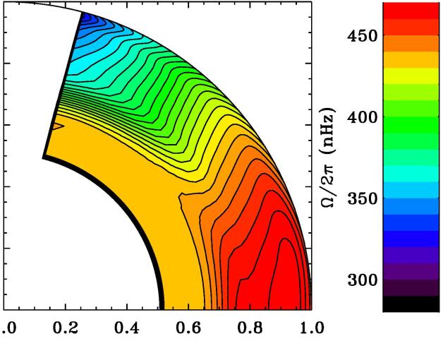
The rotation rate in much of the solar interior has been inferred from global-mode frequency splittings. A typical result for the mean rotation profile, in this case using a Regularized Least Squares (RLS) inversion technique applied to data obtained with the HMI instrument on board SDO, is shown in Fig. 6. The latitudinal variation of the rotation rate that has long been observed at the surface of the Sun, with the rotation rate decreasing with increasing latitude, is seen to persist through the convection zone (the outer 30 per cent of the Sun). Near the base of the convection zone, there is a transition to what appears to be an essentially uniform rotation rate beneath, so that at the interface there is a region of strong rotational shear which has become known as the tachocline. There is also a region of rotational shear much closer to the Sun’s surface, in about the outer five per cent by radius, so the maximum in the rotation rate occurs a few per cent beneath the surface. As remarked by Gilman and Howe (2003), in much of the convection zone the contours of isorotation make an angle with the rotation axis of about 25∘, whereas there is a slight tendency for them to align parallel to the rotation axis (“rotation on cylinders”) in the near-equatorial region (Howe et al., 2005).
5.3 Observations of torsional oscillations
There are temporal variations around the mean rotation profile. The most firmly established of these are the so-called torsional oscillations. At low latitudes, these manifest as weak but coherent bands of faster and slower rotation that start at mid-latitudes as, or even slightly before, sunspots appear at those latitudes during the solar cycle, and migrate equatorwards with the activity bands over a period of a few years. Helioseismology shows that these bands extend in depth at least a third of a way down into the convection zone (Antia and Basu, 2000; Howe et al., 2000; Vorontsov et al., 2002; Howe et al., 2006b). At high latitudes, helioseismology has revealed that there is a poleward-migrating branch of the torsional oscillation (Antia and Basu, 2001; Vorontsov et al., 2002), which may extend over the whole depth of the convection zone. The signal is clearest in the near-surface layers: Fig. 7 shows the torsional oscillations at a depth of one per cent of the solar radius beneath the surface. As these results are based on global helioseismology they do not reflect any differences between the flows in northern and southern hemispheres.
The torsional oscillation was first observed in surface Doppler observations from Mount Wilson (Howard and Labonte, 1980). These observations continued until very recently, and have been compared with the helioseismic observations by Howe et al. (2006a); when the Doppler observations are symmetrized across the equator the agreement makes it clear that the two techniques are detecting the same phenomenon. The better resolution of the helioseismic measurements at high latitudes makes the poleward-propagating nature of the high-latitude branch more obvious.
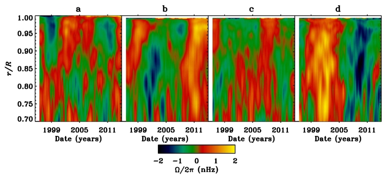
A complementary view on torsional oscillations is obtained by looking at the same results but as a function of time and depth at fixed latitude. Four such slices, at different latitudes, are shown in Fig. 8. At the equator and at latitude, there is some hint in the first half of the time period that the torsional oscillation propagates upwards from the middle of the convection zone. At the higher latitudes, there seems to be no propagation in depth. In the second half of the period there is much weaker evidence for upward propagation, although there is still some hint of it at latitude.
5.4 Flows around active regions
Convection motions manifest themselves at the Sun’s surface and in the subsurface regions on a range of scales. Moreover, strong magnetic fields in sunspots and active regions modify those convective motions, and the maintenance and decay of sunspots likely involves an interplay between the magnetic field and the flows. These flows have been studied using various local helioseismic techniques: with time-distance helioseismology (Gizon et al., 2001), ring analysis (Hindman et al., 2009) and helioseismic holography (Braun and Wan, 2011). Fig. 9 shows flows around and beneath an active region, obtained from ring analysis data derived from HMI observations. The inversion method employed is a 3-D RLS inversion developed by Featherstone et al. (2011). At the shallowest depths (0.2 Mm), the flows are dominated by the supergranular convection, and that scale is clearly visible. The flow speeds decrease with increasing depth, and the horizontal scale of the convective motions increases.
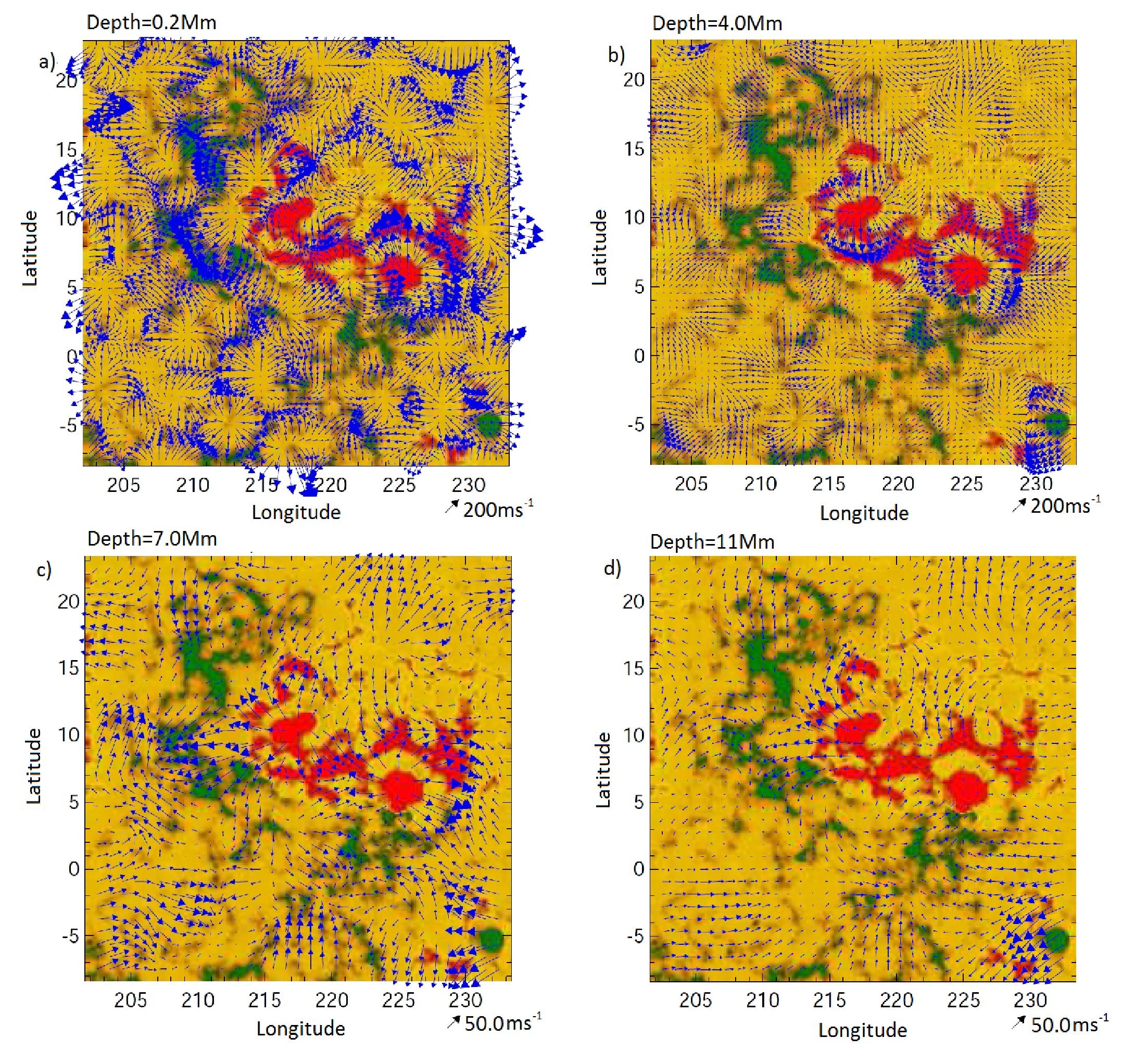
Featherstone et al. also find that strong outflows are typical around sunspots at a depth of 5-6 Mm. Comparable studies with time-distance helioseismology (Gizon et al., 2009) agree roughly with the ring-analysis studies in terms of the magnitude of surface flows near sunspots. They are also in agreement that there are strong outflows beneath the surface, but time-distance helioseismology finds that the flow speeds are higher, by about a factor of two. Resolution differences may account for some of the apparent discrepancy.
5.5 Meridional circulation: a shallow return flow?
Meridional circulation is the large-scale flow in meridional planes – i.e., flows that are perpendicular to the rotational flow. Meridional circulation in the solar convection zone is an important ingredient in some models of the solar dynamo: in the near-surface regions it transports the remnant flux from old active regions polewards, where the flux is presumed to be subducted and carried down to the bottom of the convection zone, where again a suitably directed meridional circulation may aid the equatorward migration of toroidal magnetic field.
The meridional circulation near the surface of the Sun is only of order 10 m/s, much smaller than the rotation speed and the speeds of convective motions of granules, etc. Hence, although there were pre-helioseismology surface measurements of poleward meridional flow at the surface, these measurements were difficult. In an early application of time-distance helioseismology, Giles et al. (1997) demonstrated that the near sub-surface meridional circulation in both hemispheres is polewards.
Following earlier pioneering attempts by Patron et al. (1995), Haber and colleagues have applied the ring analysis method extensively to obtain robust results regarding the meridional circulation in the outer few percent of the solar interior from the equator to nearly 60∘ latitude, e.g. Haber et al. (2002). The results show that the meridional circulation is generally poleward in this region. With a lesser degree of certainty, Haber and collaborators find that there are episodes when a submerged counter-flow develops at mid-latitudes.
As well as the possible development of a counter-cell, there are other temporal variations of the meridional circulation in the superficial subsurface layers that appear to be associated spatially and temporally with the torsional oscillations (Zhao and Kosovichev, 2004; González Hernández et al., 2010)
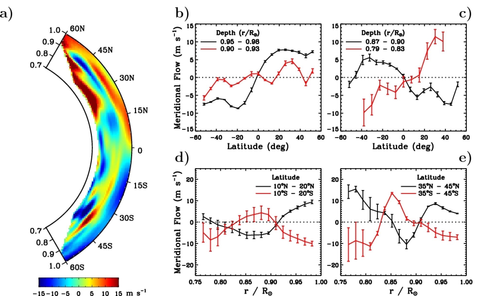
Mass conservation demands that, corresponding to the poleward near-surface meridional flow, there must be an equatorward flow at some depth that closes the circulation. The location of this return flow is a key question in determining how and whether the flux-transport solar dynamo model operates. Ever since the work by Giles et al. (1997), there have been attempts that have hinted at a relatively shallow return flow. Mitra-Kraev and Thompson (2007) detected a transition from poleward to equatorward flow at a depth of about 35 Mm, though with substantial error bars on the flow speeds. Hathaway (2012), using a cross-correlation method to track supergranules, found that the poleward meridional flow extends to about 50 Mm beneath the solar surface and reported a positive detection of equatorward flow at a depth of about 70 Mm. More recently still, arguably the most convincing helioseismic detection to date of a shallow return flow is the work by Zhao et al. (2013). These authors find that the poleward flow extends to about 0.91 (about 63 Mm depth) with an equatorward flow between 0.82 and 0.91, with perhaps a poleward flow again below that, see panel a) in Fig. 10. However, even with the latest work, a note of caution is warranted. The result depends on the application of a correction for a systematic center-to-limb bias in the travel-time measurements: the correction seems justified from a data-analysis viewpoint, but as yet the origin of the systematic is not understood.
5.6 Hemispheric Asymmetry: Flows and Magnetic Field Distribution
The solar cycle appears to be strongly coupled across the equator as evident in the symmetry of the butterfly diagram. However, a snapshot of the Sun at any given time shows notable differences between the North (N) and South (S). Usually, the hemispheric asymmetry is most notable in the distribution of the surface magnetic field but it is also observed in flows recovered from local helioseismology. So the question arises - by what mechanism are the N and S hemispheres coupled?
Passive diffusion across the geometric equator is often considered the main mechanism of coupling (Charbonneau, 2005). Results from dynamo simulations cause us to question magnetic diffusion (including turbulent diffusion) as the main coupling mechanism. Not only do the diffusion values incorporated into numerical models vary widely, the implementation as a function of depth and the effects of diffusion within the models are not well understood. Therefore, interest has been increasing regarding other, more active, hemispheric coupling mechanisms. N-S flows within latitudinally elongated convective cells (aka “banana cells”) allow a mixing of electromagnetic flux from one hemisphere into the other (Passos and Charbonneau, 2014, submitted to A&A) and can contribute to hemispheric coupling.
Local helioseismology techniques, such as ring diagram (Hill, 1989) and time-distance (Duvall et al., 1993) analysis, are able to determine non-symmetric latitudinal structure in the solar interior. Results from local heliosesmology highlight the differences in the hemispheric flows. These analyses have been used to measure distinct hemispheric differences in the meridional flows and zonal flows at a given time and depth in the interior (see Komm et al., 2011, and others). These measured asymmetries provide further quantitative constraints on the dynamo simulations in that the simulations must reproduce hemispheric asymmetries only within the range observed.
Specifically, the extent of hemispheric coupling as determined by surface magnetism is as follows. The N and S polar fields reverse their dominant polarity at distinctly different times, up to 14 months apart in some solar cycles (Norton and Gallagher, 2010). The time of peak sunspot production of one hemisphere is usually lagged by the other, meaning the hemispheres experience solar maxima at different times. Recently, the first half of the 2014 calendar year shows the Southern hemisphere producing significantly more large active regions while the Northern hemisphere peaked in sunspot production earlier in 2013. The amplitudes of each hemispheric solar cycle as measured in sunspot number or area are within 20% of each other and the timing (phase lags) between hemispheres are not more than 25% of the total cycle length (Norton and Gallagher, 2010). For more recent, in-depth analysis, Zolotova et al. (2010) and McIntosh et al. (2013) both analyze hemispheric asymmetry and interestingly enough find that a certain hemisphere appears to lead any given cycle and this lead persists for roughly 40 years on average. That is the surface magnetism characteristic of the hemispheric asymmetry.
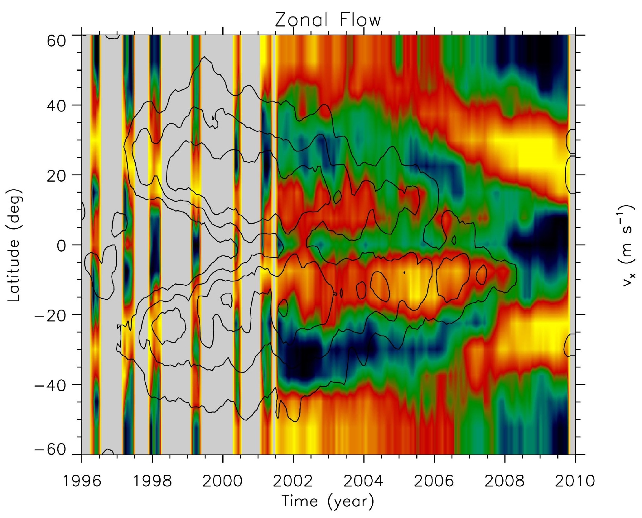
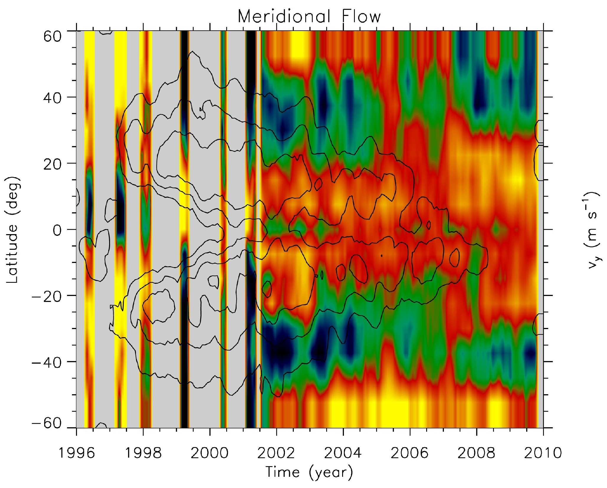
The extent of the hemispheric coupling as determined by helioseismology is as follows. Zonal flows are seen as bands of faster and slower E-W flows that appear years prior to the appearance of activity on the solar surface. It is often thought that the flow patterns are caused by enhanced cooling by magnetic fields. Meridional flows are considered in many dynamo models as the crucial ingredient which sets the rate at which the toroidal magnetic band (and sunspots) move equatorward. Komm et al. (2011) determined the zonal and meridional flows as a function of latitude for cycle 23 (years 1996-2010), see Fig. 11. In the right panel of Fig. 11, note how the meridional flow at 10-15 Mm in the Northern hemisphere weakens in 2005 at 35 N latitude (seen as a break in green color) just before the Northern surface magnetic contour disappears in 2006. Similarly, the Southern hemisphere shows this behavior 2 years later in 2007 at 35 S latitude (again, a break in the green color) just before the Southern magnetic contour disappears in 2008. This year hemispheric phase lag observed in both the surface magnetism and the meridional flow is tantalizing.
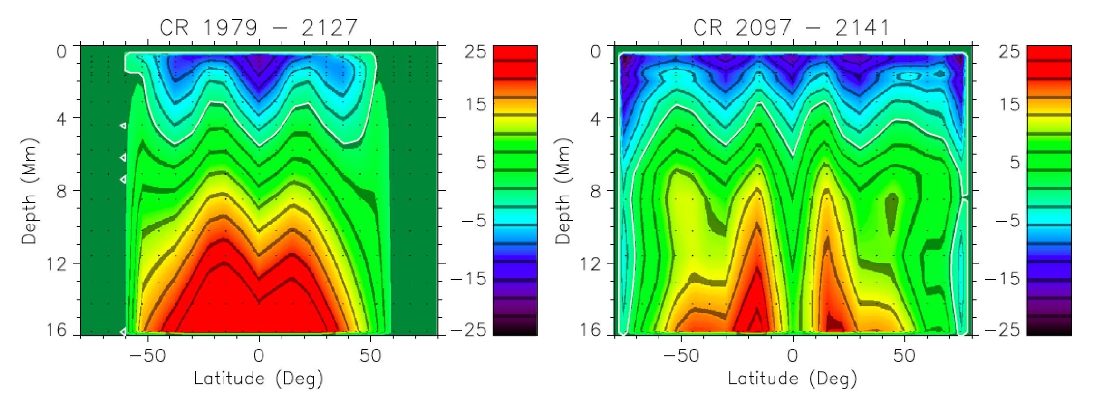
More recently, Komm et al. (2014) investigated the behavior of the zonal flows as a function of latitude for the time period of 2001 - 2013 from the surface to a depth of 16 Mm using GONG and HMI. Many hemispheric differences are evident in the zonal flows. For example, see Fig. 12 showing the poleward branch of the zonal flow (at 50 degrees) is 6 m s-1 faster in the S than the N at a depth of 10 13 Mm during cycle 23. In addition, Zhao et al. (2013) detected multiple cells in each hemisphere in the meridional circulation using acoustic travel-time differences. The double-celled profile shows a significant hemispheric asymmetry (see panels (d) and (e) in Fig. 10) in a range of latitudes. The profile asymmetry could be due to a phase lag in the hemispheres: does the meridional profile as a function of depth in the Southern hemisphere in 2013 look like the profile did in the Northern hemisphere two years earlier?
It is possible that a perturbation of meridional flow (presumably by convection since the meridional flow is a weak flow strongly driven by convection) in one hemisphere (but not in the other) sets a phase lag between the migration of activity belts, and hence, the sunspot production, that persists for years. Actively searching for correlated hemispheric asymmetric signatures in flows at depth and magnetic field distributions on the surface may provide insight as to which ingredients of the dynamo set the length and amplitude of the sunspot cycle. For an in-depth discussion of N-S hemispheric asymmetry from an observational perspective as compared to the results from dynamo simulations, see Norton et al. (2014) in this volume.
6 Mean field modelling of solar torsional oscillations
Several authors (Durney, 2000; Covas et al., 2000; Bushby, 2006; Rempel, 2006) have developed theoretical models of torsional oscillations, the observational aspects of which are described in Section 5.3, by assuming that the torsional oscillations are driven by the Lorentz force of the Sun’s cyclically varying magnetic field, which is associated with sunspot cycle. If this is true, then one would expect the torsional oscillations to follow the sunspot cycles. The puzzling fact, however, is that the torsional oscillations of a cycle begin a couple of years before the sunspots of that cycle appear and at a latitude higher than where the first sunspots are subsequently seen. At first sight, this looks like a violation of causality. How does the effect precede the cause? The following section provides a possible explanation using the Nandy-Choudhuri hypothesis (Nandy and Choudhuri, 2002) in the framework of flux transport dynamos.
6.1 Features of solar torsional oscillations and their possible explanations
We now summarize some of the other important characteristics of torsional oscillations, which a theoretical model should try to explain.
-
1.
Apart from the weaker equatorward-propagating branch which moves with the sunspot belt after the sunspots start appearing, there is also a stronger poleward-propagating branch at high latitudes. The poleward branch lasts for about 9 years whereas the equatorward branch lasts for about 18 years (e.g. see Fig. 7).
-
2.
The amplitude of the torsional oscillations near the surface is of the order of 4 nHz (20 ms-1) when averaged over all latitudes (e.g. see Fig. 7).
- 3.
-
4.
In the equatorward-propagating branch at low latitudes, the torsional oscillations at the surface seem to have a phase lag of about 2 yr compared to the oscillations at the bottom of the convection zone (see Fig. 7 in Howe et al., 2005, and Fig. 8 here). The rate of upward movement appears to be about 0.05 yr-1 or . However, we recall from Section 5.3 that evidence for upward propagation is weaker in cycle 24 than observed previously.
- 5.
Let us now try to understand properties (3) and (4) listed above in some more detail. Property (4) of the torsional oscillations seems to suggest that the bottom of the convection zone is the source of the oscillations, which then propagate upwards. Property (3) then seems puzzling and contrary to common sense. One would expect the oscillations to be more coherent near the source, becoming more diffuse as they move upward further away from the source. However, we know that the magnetic field is highly intermittent within the convection zone and we need to take account of this fact when calculating the Lorentz force due to the magnetic field. Since the convection cells deeper down are expected to have larger sizes, Choudhuri (2003) suggested that the magnetic field within the convection zone would look as shown in Fig. 1 of that paper. In Fig. 1 of Choudhuri the convection granule size is a function of the pressure scale height in the solar convection zone, the intergranular lanes are more intermittent at the bottom of the convection zone and so is the magnetic field which is concentrated into tubes in these lanes. Since the velocity perturbations associated with the torsional oscillations are likely to be concentrated around the magnetic flux tubes, we expect the torsional oscillations to be spatially intermittent at the bottom of the convection zone, as seen in the observational data (property 3). Similarly, since the magnetic field near the surface is less intermittent, a torsional oscillation driven by the Lorentz stress would also appear more coherent there. This may explain the puzzling situation where the torsional oscillations seem to become more coherent as they move further away from the source which is at the footpoints of flux tubes at the bottom of the convection zone. This scenario therefore provides a natural explanation for property (3) of the torsional oscillations, as listed above. Accordingly, let us assume that the torsional oscillation gets initiated in the lower footpoints of the vertical flux tubes, where the Lorentz force builds up due to the production of the toroidal magnetic field. This perturbation then propagates upward along the vertical flux tubes at the Alfvén speed. If the magnetic field inside the flux tubes within the solar convection zone (not below it) is estimated as 500 G (see Section 3 of Choudhuri (2003)), then the Alfvén speed at the bottom of the convection zone is of the order of 300 cm s-1 and the Alfvén travel time from the bottom to the top turns out to be exactly of the same order as the phase delay of torsional oscillations at the surface compared to the oscillations at the bottom of the convection zone. This may be an explanation for the property (4). In the next subsection, we shall try to incorporate these ideas into a mean field dynamo model of the solar cycle.
6.2 Numerical Modelling efforts
We focus on the scenario where the Lorentz and MAxwell stresses on the flows in the solar interior give rise to the torsional oscillations. Poloidal flows, like the meridional circulation, are also affected. This is important because the meridional circulation is believed to set the clock for the 11yr sunspot cycle. The magnetic feedback on the flows is one of the important non linearities of the solar dynamo. Some authors have proposed that such feedback on differential rotation alone could cause a modulation of solar cycle strengths and lead to grand minima like episodes (Kitchatinov et al., 1999).
Mean field models of the solar dynamo have been in existence for over two decades now and come in two main flavors: the , interface, and the flux transport dynamo. Depending on the values of parameters like turbulent diffusivity as compared to meridional circulation speed, the dynamo can also be characterized into advectively or diffusively dominated dynamo regimes (Jiang et al., 2007; Yeates et al., 2008). Such a mean field model of the solar dynamo can then be combined with the Reynolds-averaged Navier-Stokes (NS) equation, after including the effects of the Lorentz force and Maxwells stresses, to solve for the torsional oscillations. Several authors (Covas et al., 2000, 2004; Chakraborty et al., 2009) have solved for only the azimuthal component of the mean velocity, along with the dynamo equations while others (Rempel, 2007) have solved for the evolution of entropy in addition to all three components of the mean velocity. Torsional oscillation models also differ in relation to the magnetic feedback term appearing in the NS equation. In some cases (Rempel, 2007; Chakraborty et al., 2009; Covas et al., 2004) only a Lorentz feedback due to the mean magnetic field (macro-feedback), has been used whereas in other cases (Kitchatinov et al., 1999; Küker et al., 1999) only the Maxwell’s stress due to the fluctuating magnetic field (micro-feedback) has been modeled. This is achieved using -effect formulation of the non-diffusive component of the Reynolds stresses (Kitchatinov and Rüdiger, 1993) and quenching the coefficients using an algebraic dependence on the mean magnetic field. The saturation of the mean magnetic field in the above case has been achieved using two different mechanisms: In the first mechanism the coefficients are quenched along with either the kinetic helicity or the effect (achieved through the presence of super equipartition fields). The second mechanism was employed by Covas et al. (2004) who demonstrated that saturation of the solar dynamo can be obtained by means of the Lorentz feedback in the component of the NS equation without requiring any explicit -quenching.
One of the popular models used for an explanation of the sunspot cycle is the flux transport dynamo, in which the meridional circulation carries the toroidal field produced from differential rotation in the tachocline equatorward and carries the poloidal field produced by the Babcock–Leighton mechanism at the surface poleward (Wang and Sheeley, 1991; Choudhuri et al., 1995). Since the differential rotation is stronger at higher latitudes in the tachocline than at lower latitudes, the inclusion of solar-like rotation tends to produce a strong toroidal field at high latitudes rather than at the latitudes where sunspots are seen (Dikpati and Charbonneau, 1999; Küker et al., 2001). Nandy and Choudhuri (2002) proposed a hypothesis to overcome this difficulty. According to their hypothesis, the meridional circulation penetrates slightly below the bottom of the convection zone and the strong toroidal field produced at the high-latitude tachocline is pushed by this meridional circulation into stable layers below the convection zone where magnetic buoyancy is suppressed and sunspots are not formed. Only when the toroidal field is brought into the convection zone by the meridional circulation rising at lower latitudes, does magnetic buoyancy take over and sunspots finally form. The torsional oscillation signals however cannot be buried below the convection zone by the meridional circulation since they can be transmitted out to the surface by Alfvén waves along vertical magnetic field lines, which intermittently thread the convection zone. It may be noted that there is a controversy at the present time as to whether the meridional circulation can penetrate below the convection zone since arguments having been advanced both against (Gilman and Miesch, 2004) and for it (Garaud and Brummel, 2008). The detailed dynamo model of Chatterjee et al. (2004) was based on this Nandy-Choudhuri hypothesis, which provided the correct sunspot emergence latitudes and phase relation between the low-latitute toroidal field and the polar fields at the surface.
Another conjecture proposed by Chakraborty et al. (2009) was that the torsional oscillations are initiated in the lower layers of the solar convection zone where toroidal flux tubes are formed due to differential rotation and are propagated upwards by Alfvén waves. The torsional oscillation signal therefore reaches the solar surface much ahead of the sunspot-forming toroidal magnetic field which is still buried by the downward meridional flow in the stable layers. These authors tried to model torsional oscillations using the Chatterjee et al. (2004) dynamo model after coupling it to the equation for the mean rotational velocity incorporating a very simple but insightful averaging of the Lorentz force feedback term. The component of the Navier–Stokes equation, is
| (6) |
where
| (7) |
is the term corresponding to advection by the meridional circulation , and is a constant upward velocity of cm s-1, estimated in Section 6.1, to account for the upward transport by Alfvén waves when solving our basic equation Eq. 6. Note that this additional does not represent any actual mass motion and does not have to satisfy the continuity equation, unlike the meridional circulation.
| (8) |
is the diffusion term, and is the component of the Lorentz force. The kinematic viscosity is primarily due to turbulence within the convection zone and is expected to be equal to the magnetic diffusivity. If the magnetic field in our model is assumed to have the standard form
| (9) |
then the Lorentz force is given by the Jacobian
| (10) |
where . We, however, have to take some special care in averaging the term in Eq. 10, since this is the only term in our equations which is quadratic in the basic variables and has to be averaged differently from all the other terms due to intermittency of the magnetic field in the convection zone. The component of the Lorentz force primarily comes from the radial derivative of the magnetic stress . This stress arises when is stretched by differential rotation to produce and should be non-zero only inside the flux tubes. We assume that are the mean field values, whereas are the values of these quantities inside flux tubes. If is the filling factor, which is essentially the fractional volume occupied by flux tubes, then we have and , on assuming the same filling factor for both components for the sake of simplicity. It is easy to see that the mean Lorentz stress would be
| (11) |
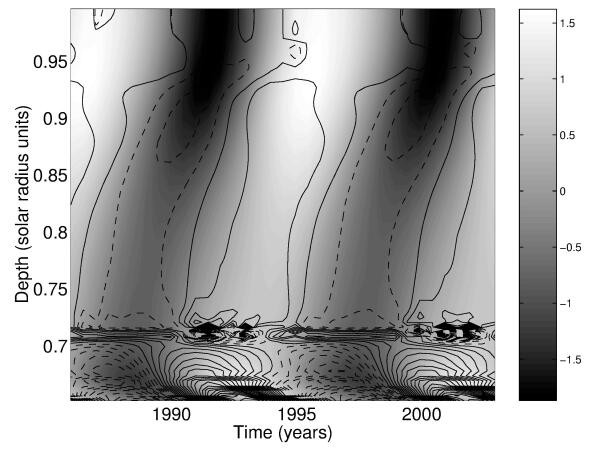
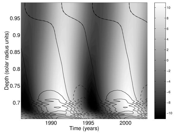
This suggests that the correct mean field expression for should be given by the Eq.10 divided by . As pointed out by Chatterjee et al. (2004), the only non-linearity in our equations comes from the critical magnetic field above which the toroidal field at the bottom of the convection zone is supposed to be unstable due to magnetic buoyancy. Jiang et al. (2007) found that we have to take G (which is the critical value of the mean toroidal field and not the toroidal field inside flux tubes) to ensure that the poloidal field at the surface has correct values. Once the amplitude of the magnetic field gets fixed in this manner, we find that the amplitude of the torsional oscillations matches observational values only for a particular value of the filling factor . The theoretical model of torsional oscillations proposed by Chakraborty et al. (2009) thus allows us to infer the filling factor of the magnetic field in the lower layers of the convection zone. Even though the conjecture of Chakraborty et al. looks very elegant, upon actual calculation they obtained a large phase lag of years instead of the observed 2 years between the onset of the low-latitude branch of the torsional oscillation and the first appearance of sunspots of the cycle. However, the radial dependence of the torsional signal was very close to the observed patterns and is shown in Fig. 13. It is clear in the plot of the torsional oscillation at a latitude of (left panel of Fig. 13) that the Lorentz force is concentrated in the tachocline at 0.7, where the low-latitude torsional oscillations are launched to propagate upward. The plot for latitude shows that the amplitude of the torsional oscillations becomes larger near the surface due to the perturbations propagating into regions of lower density, which is consistent with observational data. The physics of the high-latitude branch (right panel of Fig. 13) is, however, very different, with the Lorentz force contours indicating a downward propagation and not a particularly strong concentration at the tachocline. As the poloidal field sinks with the downward meridional circulation at the high latitudes, the latitudinal shear in the convection zone acts on it to create the toroidal component and thereby the Lorentz stress. With the downward advection of the poloidal field, the region of Lorentz stress moves downward.
Yet another baffling observation which has eluded modelers is the systematic deviation of the isolines of constant phase of the torsional oscillation from the Taylor-Proudman state, where the fluid velocity should be uniform along contours parallel to the rotation axis, as evident from Fig. 3B of Vorontsov et al. (2002). Howe et al. (2004b) first pointed out that lines of constant phase are inclined at to the rotation axis, similar to the isorotation contours. Spruit (2003) suggested a thermal origin for the low-latitude branch of the torsional oscillation due to enhanced radiative losses in the active region belts. Rempel (2007) showed that only a localized thermal forcing can lead to such deviation from the Taylor-Proudman state. However since the thermal forcing is only concentrated near the surface, it does not explain the observational fact that torsional oscillations encompass almost the entire convection zone. Earlier, Rempel (2006, see Fig. 10 of that paper) showed that applying a surface cooling function confined to sunspot emerging latitudes can give rise to the low-latitude branch of the torsional oscillation where as the magnetic forcing is responsible for the high-latitude branch. According to our knowledge none of the authors have yet obtained the correct phase relation between the low-latitude band of the torsional oscillation and the sunspot migration. The precedence of the low-latitude branch over the first appearance of sunspots is still a mystery.
Note that, all the discussion above are for mean field models which give rise to regular solar cycle amplitudes for a relatively weak magnetic feedback. An exception is the model of Kitchatinov et al. (1999) which has a strong magnetic feedback and gives rise to significant modulation in the strengths of successive solar cycles. In reality, the solar cycle amplitudes are irregular or stochastic in nature. Naturally this would give rise to an irregular magnetic feedback on the solar flows and the resulting observed torsional oscillations. The irregular magnetic feedback can not only affect the amplitude of torsional oscillations but also the mean rotation rate of the Sun. It may be important to define the mean rotation rate as a solar cycle averaged quantity rather than a very long temporal average (see Howe et al., 2013). Thus, modelling the solar torsional oscillations still remains a very challenging problem.
7 Was cycle 23 unusual?
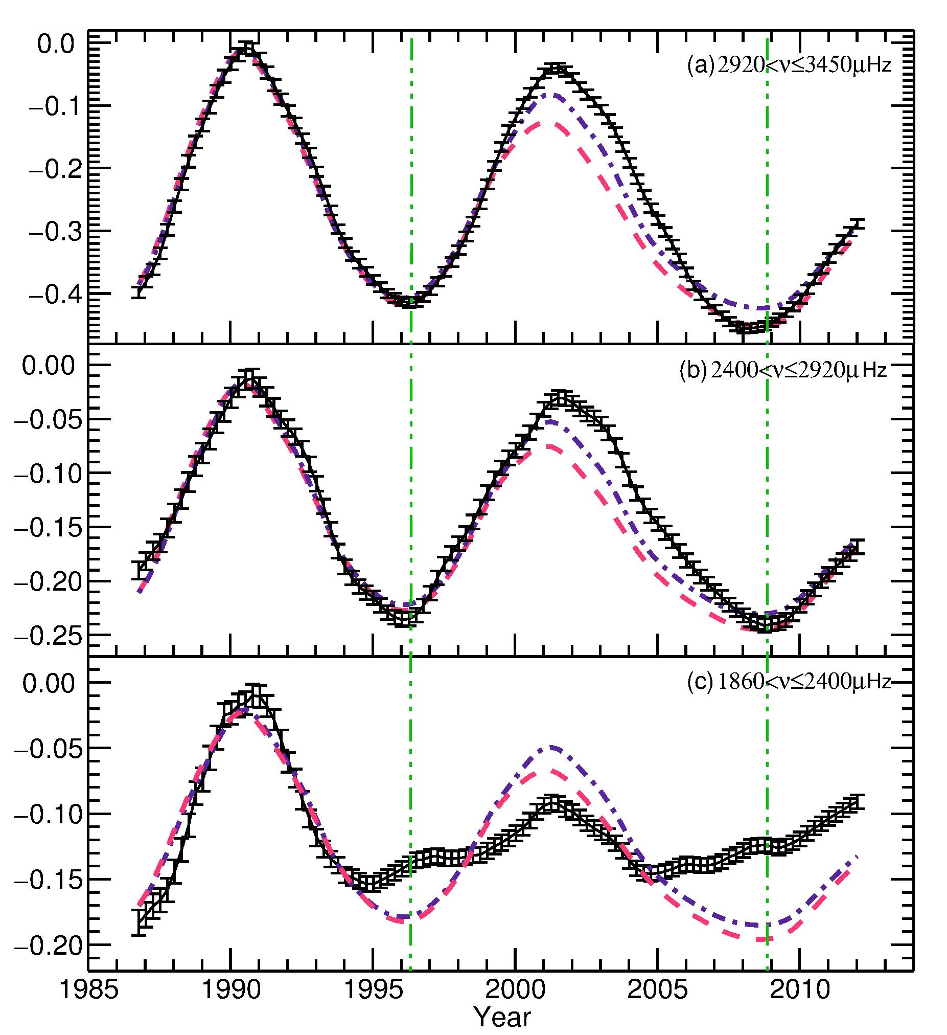
The minimum that preceded cycle 24 was considered to be unusually long and quiet, even for a solar minimum. What can the solar oscillations tell us about the structure of the Sun’s magnetic field during this time? Basu et al. (2012) examined the frequency dependence of the frequency shifts observed in Sun-as-a-star data during the last two solar cycles. Fig.14 shows the frequency shifts of low- () modes in three frequency ranges. The shifts have been smoothed to remove the quasi-biennial variation (e.g. Fletcher et al., 2010). Fig. 14 shows that the low-frequency modes behave unexpectedly, not just during the recent unusual solar minimum but for the entirety of cycle 23, experiencing little to no frequency shift during this time. Although it is expected that the low-frequency modes experience a smaller shift in frequency than the high-frequency modes (see Section 3.2), a comparison with the shifts observed in cycle 22 highlights the discrepancy. More precisely, while the behaviour of the high and intermediate ranges is consistent between cycles 22 and 23, the behaviour of the low-frequency modes changes. This can be explained in terms of the upper turning points of the modes, which as we have said previously, are dependent on the frequency of the mode. If we consider the perturbation responsible for the solar-cycle frequency shifts to be a near-surface magnetic layer. In cycle 22 the upper turning points of the low-frequency modes must lie within the magnetic layer, but in cycle 23 the upper turning points of the low frequency modes must lie beneath the layer, meaning their frequencies are not perturbed by it. These results, therefore, imply a thinning of the magnetic layer (or a change in the upper turning points with respect to the layer). Basu et al. (2012) therefore infer that the magnetic layer must be positioned above in cycle 23.
A change in behaviour has also been observed in the torsional oscillation. In Fig. 7 it appears that the high-latitude poleward-propagating spin-up, which was prominent in the 2000-2006 epoch, is absent in the present cycle. It has been speculated that the high-latitude branch is a precursor of the following solar cycle, and that its absence at the present time may indicate that cycle 25 may be delayed, weak, or non-existent. Another way to look at the data is to plot the inferred rotation at a single location, as a function of time (Fig. 15). It is clear from this representation that the rotation rate at mid- and high-latitudes has been increasing in the past 2-3 years, but more weakly than in the previous cycle. At mid-latitudes, it is also evident that the rotation rate dropped to a lower level than in the previous cycle, so even the weak increase is starting from a lower base (Howe et al., 2013).

8 Summarizing remarks
The Sun’s magnetic field, which is generated in the solar interior, varies on a time scale of 11 yrs from minimum to maximum and back again. Measures of the Sun’s surface and atmospheric magnetic field are abundant. In order to really understand the interior of the Sun we use the Sun’s natural oscillations. The frequencies, powers and lifetimes of these oscillations are dependent on the strength of the Sun’s magnetic field, with the most significant influence on the oscillations arising from a near-surface perturbation. In fact, it has been shown that the change in frequency of the oscillations is tightly correlated with the surface magnetic field, once latitudinal distribution is taken into account. Evidence for a magnetic field deeper within the solar interior was hard to come by. However, there is now tentative evidence for solar cycle variations in the second-ionization zone of helium and at the base of the convection zone. Solar cycle variations in the dynamics of the solar interior have been far more forthcoming. For example, the link between flows and active regions, such as sunspots, have been well studied and reveal strong outflows around sunspots. The torsional oscillation has been shown to exist over a substantial fraction of the convection zone. The observational constraints of the torsional oscillations have proven to be key in recent developments in mean field dynamo models. This is particularly pertinent since one of the main aims in any solar cycle study is to improve our understanding of the mechanism by which the Sun’s magnetic field is generated and maintained. Any model of the solar dynamo must explain observational features, including the North-South asymmetry, which is apparent, not only in surface measures of the Sun’s magnetic field but in the flows seen in the solar interior. Finally it has been shown that, from a helioseismic standpoint the Sun’s activity appears to be changing from one cycle to the next. We must remember here that we only have two 11-yr solar cycles for comparison. Although the BiSON data do go back to cycle 21, the fill of the data is poor as the full 6-site network was not established until the early 1990s, meaning that it is hard to make helioseismic inferences about this cycle. It is, therefore, difficult to say, purely in helioseismic terms, which cycle is behaving unusually, or indeed if the behaviour is unusual at all: 11 yr only covers half a 22-yr Hale cycle. One can, therefore, only conclude that the helioseismic data imply that the behaviour of the Sun has changed. Hopefully these and other issues surrounding the Sun’s magnetic field will become clearer as we continue to observe the Sun through cycle 24 and beyond.
Acknowledgements.
The paper was stimulated by the workshop “The solar activity cycle: physical causes and consequences”. It is a pleasure to thank André Balogh, Hugh Hudson, Kristof Petrovay, Rudolf von Steiger and the International Space Science Institute for financial support, excellent organization and hospitality. This work utilizes Birmingham Solar Oscillations Network data which is run by School of Physics and Astronomy, University of Birmingham. This work utilizes GONG data obtained by the NSO Integrated Synoptic Program (NISP), managed by the National Solar Observatory, which is operated by AURA, Inc. under a cooperative agreement with the National Science Foundation. The data were acquired by instruments operated by the Big Bear Solar Observatory, High Altitude Observatory, Learmonth Solar Observatory, Udaipur Solar Observatory, Instituto de Astrofísica de Canarias, and Cerro Tololo Interamerican Observatory. SOHO is a mission of international cooperation between ESA and NASA. The Solar Oscillations Investigation (SOI) involving MDI was supported by NASA grant NNX09AI90G to Stanford University. The National Center for Atmospheric Research is sponsored by the National Science Foundation. HMI data courtesy of NASA and the HMI consortium; HMI is supported by NASA contract NAS5-02139 to Stanford University. NSO/Kitt Peak data used here were produced cooperatively by NSF/NOAO, NASA/GSFC, and NOAA/SEL; SOLIS data are produced cooperatively by NSF/NSO and NASA/LWS. A-MB thanks the Institute of Advanced Study, University of Warwick for their support. RH acknowledges computing support from the National Solar Observatory. A. Norton is supported by NASA Contract NAS5-02139 (HMI) to Stanford University. We thank N. Featherstone and R. Komm for their help.References
- Anguera Gubau et al. (1992) M. Anguera Gubau, P.L. Palle, F. Perez Hernandez, C. Regulo, T. Roca Cortes, The low L solar p-mode spectrum at maximum and minimum solar activity. A&A 255, 363–372 (1992)
- Antia and Basu (2000) H.M. Antia, S. Basu, Temporal Variations of the Rotation Rate in the Solar Interior. ApJ 541, 442–448 (2000). doi:10.1086/309421
- Antia et al. (2000) H.M. Antia, S.M. Chitre, M.J. Thompson, The Sun’s acoustic asphericity and magnetic fields in the solar convection zone. A&A 360, 335–344 (2000)
- Antia et al. (2001) H.M. Antia, S. Basu, F. Hill, R. Howe, R.W. Komm, J. Schou, Solar-cycle variation of the sound-speed asphericity from GONG and MDI data 1995-2000. MNRAS 327, 1029–1040 (2001). doi:10.1046/j.1365-8711.2001.04819.x
- Antia and Basu (2001) H.M. Antia, S. Basu, Temporal variations of the solar rotation rate at high latitudes. ApJL 559, 67–70 (2001). doi:10.1086/323701
- Appourchaux (2001) T. Appourchaux, Results from the luminosity oscillations imager on board SOHO: low-degree p-mode parameters for a 4-year data set, in SOHO 10/GONG 2000 Workshop: Helio- and Asteroseismology at the Dawn of the Millennium, ed. by A. Wilson, P.L. Pallé ESA Special Publication, vol. 464, 2001, pp. 71–74
- Baldner and Basu (2008) C.S. Baldner, S. Basu, Solar Cycle Related Changes at the Base of the Convection Zone. ApJ 686, 1349–1361 (2008). doi:10.1086/591514
- Baldner et al. (2009) C.S. Baldner, T.P. Larson, S. Basu, Solar-Cycle Related Changes at the Base of the Convection Zone, in Solar-Stellar Dynamos as Revealed by Helio- and Asteroseismology: GONG 2008/SOHO 21, ed. by M. Dikpati, T. Arentoft, I. González Hernández, C. Lindsey, F. Hill Astronomical Society of the Pacific Conference Series, vol. 416, 2009, p. 477
- Balmforth et al. (1996) N.J. Balmforth, D.O. Gough, W.J. Merryfield, Structural changes to the Sun through the solar cycle. MNRAS 278, 437–448 (1996)
- Basu (1997) S. Basu, Seismology of the base of the solar convection zone. MNRAS 288, 572–584 (1997)
- Basu (2002) S. Basu, What does helioseismology tell us about solar cycle related structural changes in the Sun?, in From Solar Min to Max: Half a Solar Cycle with SOHO, ed. by A. Wilson ESA Special Publication, vol. 508, 2002, pp. 7–14
- Basu and Antia (2000) S. Basu, H.M. Antia, Possible solar cycle variations in the convection zone. Sol. Phys. 192, 449–458 (2000). doi:10.1023/A:1005232901528
- Basu and Antia (2001) S. Basu, H.M. Antia, A study of possible temporal and latitudinal variations in the properties of the solar tachocline. MNRAS 324, 498–508 (2001). doi:10.1046/j.1365-8711.2001.04364.x
- Basu and Antia (2003) S. Basu, H.M. Antia, Temporal variations of solar structure, in GONG+ 2002. Local and Global Helioseismology: the Present and Future, ed. by H. Sawaya-Lacoste ESA Special Publication, vol. 517, 2003, pp. 231–234
- Basu and Mandel (2004) S. Basu, A. Mandel, Does Solar Structure Vary with Solar Magnetic Activity? ApJL 617, 155–158 (2004). doi:10.1086/427435
- Basu and Schou (2000) S. Basu, J. Schou, Does the tachocline show solar cycle related changes? Sol. Phys. 192, 481–486 (2000). doi:10.1023/A:1005231509224
- Basu et al. (1994) S. Basu, H.M. Antia, D. Narasimha, Helioseismic measurement of the extent of overshoot below the solar convection zone. MNRAS 267, 209 (1994)
- Basu et al. (2003) S. Basu, J. Christensen-Dalsgaard, R. Howe, J. Schou, M.J. Thompson, F. Hill, R. Komm, A Comparison of Solar p-Mode Parameters from MDI and GONG: Mode Frequencies and Structure Inversions. ApJ 591, 432–445 (2003). doi:10.1086/375331
- Basu et al. (2012) S. Basu, A.-M. Broomhall, W.J. Chaplin, Y. Elsworth, Thinning of the Sun’s Magnetic Layer: The Peculiar Solar Minimum Could Have Been Predicted. ApJ 758, 43 (2012). doi:10.1088/0004-637X/758/1/43
- Berrilli et al. (1999) F. Berrilli, I. Ermolli, A. Florio, E. Pietropaolo, Average properties and temporal variations of the geometry of solar network cells. A&A 344, 965–972 (1999)
- Bogart et al. (2008) R.S. Bogart, S. Basu, M.C. Rabello-Soares, H.M. Antia, Probing the Subsurface Structures of Active Regions with Ring-Diagram Analysis. Sol. Phys. 251, 439–451 (2008). doi:10.1007/s11207-008-9213-9
- Braun and Wan (2011) D.C. Braun, K. Wan, Properties of Near-surface Flows around Active Regions from Helioseismic Holography. Journal of Physics Conference Series 271(1), 012007 (2011). doi:10.1088/1742-6596/271/1/012007
- Broomhall et al. (2009) A. Broomhall, W.J. Chaplin, Y. Elsworth, S.T. Fletcher, R. New, Is the Current Lack of Solar Activity Only Skin Deep? ApJL 700, 162–165 (2009). doi:10.1088/0004-637X/700/2/L162
- Brown et al. (1992) T.M. Brown, T.J. Bogdan, B.W. Lites, J.H. Thomas, Localized sources of propagating acoustic waves in the solar photosphere. ApJL 394, 65–68 (1992). doi:10.1086/186473
- Burtseva et al. (2009) O. Burtseva, F. Hill, S. Kholikov, D. Chou, Lifetimes of High-Degree p Modes in the Quiet and Active Sun. Sol. Phys. 258, 1–11 (2009). doi:10.1007/s11207-009-9399-5
- Bushby (2006) P.J. Bushby, Zonal flows and grand minima in a solar dynamo model. MNRAS 371, 772 (2006)
- Cally (1995) P.S. Cally, Effects of Weak-to-Moderate Vertical Magnetic Fields on Solar f- and p-Modes. ApJ 451, 372 (1995). doi:10.1086/176226
- Chakraborty et al. (2009) S. Chakraborty, A.R. Choudhuri, P. Chatterjee, Why Does the Sun’s Torsional Oscillation Begin before the Sunspot Cycle? Physical Review Letters 102(4), 041102 (2009). doi:10.1103/PhysRevLett.102.041102
- Chaplin et al. (1996) W.J. Chaplin, Y. Elsworth, R. Howe, G.R. Isaak, C.P. McLeod, B.A. Miller, H.B. van der Raay, S.J. Wheeler, R. New, BiSON Performance. Sol. Phys. 168, 1–18 (1996). doi:10.1007/BF00145821
- Chaplin et al. (1998) W.J. Chaplin, Y. Elsworth, G.R. Isaak, R. Lines, C.P. McLeod, B.A. Miller, R. New, An analysis of solar p-mode frequencies extracted from BiSON data: 1991-1996. MNRAS 300, 1077–1090 (1998)
- Chaplin et al. (2000) W.J. Chaplin, Y. Elsworth, G.R. Isaak, B.A. Miller, R. New, Variations in the excitation and damping of low-l solar p modes over the solar activity cycle. MNRAS 313, 32–42 (2000). doi:10.1046/j.1365-8711.2000.03176.x
- Chaplin et al. (2001) W.J. Chaplin, T. Appourchaux, Y. Elsworth, G.R. Isaak, R. New, The phenomenology of solar-cycle-induced acoustic eigenfrequency variations: a comparative and complementary analysis of GONG, BiSON and VIRGO/LOI data. MNRAS 324, 910–916 (2001). doi:10.1046/j.1365-8711.2001.04357.x
- Chaplin et al. (2003) W.J. Chaplin, Y. Elsworth, G.R. Isaak, B.A. Miller, R. New, S. Thiery, P. Boumier, A.H. Gabriel, Observation of, and temporal variations in, solar p-mode multiplet frequency asymmetries at l= 2. MNRAS 343, 343–352 (2003). doi:10.1046/j.1365-8711.2003.06686.x
- Chaplin et al. (2004a) W.J. Chaplin, T. Appourchaux, Y. Elsworth, G.R. Isaak, B.A. Miller, R. New, On comparing estimates of low-l solar p-mode frequencies from Sun-as-a-star and resolved observations. A&A 424, 713–717 (2004a). doi:10.1051/0004-6361:20040501
- Chaplin et al. (2004b) W.J. Chaplin, Y. Elsworth, G.R. Isaak, B.A. Miller, R. New, The solar cycle as seen by low-l p-mode frequencies: comparison with global and decomposed activity proxies. MNRAS 352, 1102–1108 (2004b). doi:10.1111/j.1365-2966.2004.07998.x
- Chaplin et al. (2007) W.J. Chaplin, Y. Elsworth, B.A. Miller, G.A. Verner, R. New, Solar p-Mode Frequencies over Three Solar Cycles. ApJ 659, 1749–1760 (2007). doi:10.1086/512543
- Charbonneau (2005) P. Charbonneau, A Maunder Minimum Scenario Based on Cross-Hemispheric Coupling and Intermittency. Sol. Phys. 229, 345–358 (2005). doi:10.1007/s11207-005-8150-0
- Charbonneau (2010) P. Charbonneau, Dynamo Models of the Solar Cycle. Living Reviews in Solar Physics 7, 3 (2010). doi:10.12942/lrsp-2010-3
- Chatterjee et al. (2004) P. Chatterjee, D. Nandy, A.R. Choudhuri, Full-sphere simulations of a circulation-dominated solar dynamo: Exploring the parity issue. A&A 427, 1019–1030 (2004)
- Chou and Serebryanskiy (2005) D.-Y. Chou, A. Serebryanskiy, In Search of the Solar Cycle Variations of p-Mode Frequencies Generated by Perturbations in the Solar Interior. ApJ 624, 420–427 (2005). doi:10.1086/428925
- Choudhuri (2003) A.R. Choudhuri, On the connection between mean field dynamo theory and flux tubes. Sol. Phys. 215, 31–55 (2003)
- Choudhuri et al. (1995) A.R. Choudhuri, M. Schussler, M. Dikpati, The solar dynamo with meridional circulation. A&A 303, 29 (1995)
- Christensen-Dalsgaard and Berthomieu (1991) J. Christensen-Dalsgaard, G. Berthomieu, Theory of solar oscillations. (Solar Interior and Atmosphere, 1991), pp. 401–478
- Christensen-Dalsgaard et al. (2011) J. Christensen-Dalsgaard, M.J.P.F.G. Monteiro, M. Rempel, M.J. Thompson, A more realistic representation of overshoot at the base of the solar convective envelope as seen by helioseismology. MNRAS 414, 1158–1174 (2011). doi:10.1111/j.1365-2966.2011.18460.x
- Covas et al. (2004) E. Covas, D. Moss, R. Tavakol, The influence of density stratification and multiple nonlinearities on solar torsional oscillations. A&A 416, 775–782 (2004). doi:10.1051/0004-6361:20034046
- Covas et al. (2000) E. Covas, R. Tavakol, D. Moss, A. Tworkowski, Torsional oscillations in the solar convection zone. A&A 360, 21–24 (2000)
- Cox (1980) J.P. Cox, Theory of stellar pulsation 1980
- Dikpati and Charbonneau (1999) M. Dikpati, P. Charbonneau, A Babcock-Leighton Flux Transport Dynamo with Solar-like Differential Rotation. ApJ 518, 508–520 (1999)
- Durney (2000) B..R. Durney, ”on the torsional oscillations in babcock-leighton solar dynamo models”. Sol. Phys. 196, 1 (2000)
- Duvall et al. (1993) T.L. Duvall Jr., S.M. Jefferies, J.W. Harvey, M.A. Pomerantz, Time-distance helioseismology. Nature 362, 430–432 (1993). doi:10.1038/362430a0
- Dziembowski and Goode (1992) W.A. Dziembowski, P.R. Goode, Effects of differential rotation on stellar oscillations - A second-order theory. ApJ 394, 670–687 (1992). doi:10.1086/171621
- Dziembowski and Goode (2005) W.A. Dziembowski, P.R. Goode, Sources of Oscillation Frequency Increase with Rising Solar Activity. ApJ 625, 548–555 (2005). doi:10.1086/429712
- Eff-Darwich et al. (2002) A. Eff-Darwich, S.G. Korzennik, S.J. Jiménez-Reyes, F. Pérez Hernández, An Upper Limit on the Temporal Variations of the Solar Interior Stratification. ApJ 580, 574–578 (2002). doi:10.1086/343063
- Elsworth et al. (1990) Y. Elsworth, R. Howe, G.R. Isaak, C.P. McLeod, R. New, Variation of low-order acoustic solar oscillations over the solar cycle. Nature 345, 322–324 (1990). doi:10.1038/345322a0
- Elsworth et al. (1993) Y. Elsworth, R. Howe, G.R. Isaak, C.P. McLeod, B.A. Miller, C.C. Speake, S.J. Wheeler, R. New, The variation in the strength of low-l solar p-modes - 1981-92. MNRAS 265, 888 (1993)
- Elsworth et al. (1994) Y. Elsworth, R. Howe, G.R. Isaak, C.P. McLeod, B.A. Miller, R. New, C.C. Speake, S.J. Wheeler, Solar p-mode frequencies and their dependence on solar activity recent results from the BISON network. ApJ 434, 801–806 (1994). doi:10.1086/174783
- Elsworth et al. (1995) Y. Elsworth, R. Howe, G.R. Isaak, C.P. McLeod, B.A. Miller, R. New, S.J. Wheeler, Techniques used in the analysis of solar oscillations data from the BiSON (University of Birmingham) network. I. Daily calibration. A&AS 113, 379 (1995)
- Featherstone et al. (2011) N.A. Featherstone, B.W. Hindman, M.J. Thompson, Ring-analysis flow measurements of sunspot outflows. Journal of Physics Conference Series 271(1), 012002 (2011). doi:10.1088/1742-6596/271/1/012002
- Fletcher et al. (2010) S.T. Fletcher, A. Broomhall, D. Salabert, S. Basu, W.J. Chaplin, Y. Elsworth, R.A. García, R. New, A Seismic Signature of a Second Dynamo? ApJL 718, 19–22 (2010). doi:10.1088/2041-8205/718/1/L19
- Foullon and Roberts (2005) C. Foullon, B. Roberts, The influence of internal magnetic layers on the frequencies of solar p-modes. A&A 439, 713–726 (2005). doi:10.1051/0004-6361:20041910
- Fröhlich et al. (1995) C. Fröhlich, J. Romero, H. Roth, C. Wehrli, B.N. Andersen, T. Appourchaux, V. Domingo, U. Telljohann, G. Berthomieu, P. Delache, J. Provost, T. Toutain, D.A. Crommelynck, A. Chevalier, A. Fichot, W. Däppen, D. Gough, T. Hoeksema, A. Jiménez, M.F. Gómez, J.M. Herreros, T.R. Cortés, A.R. Jones, J.M. Pap, R.C. Willson, VIRGO: Experiment for Helioseismology and Solar Irradiance Monitoring. Sol. Phys. 162, 101–128 (1995). doi:10.1007/BF00733428
- Gabriel et al. (1995) A.H. Gabriel, G. Grec, J. Charra, J. Robillot, T. Roca Cortés, S. Turck-Chièze, R. Bocchia, P. Boumier, M. Cantin, E. Cespédes, B. Cougrand, J. Crétolle, L. Damé, M. Decaudin, P. Delache, N. Denis, R. Duc, H. Dzitko, E. Fossat, J. Fourmond, R.A. García, D. Gough, C. Grivel, J.M. Herreros, H. Lagardère, J. Moalic, P.L. Pallé, N. Pétrou, M. Sanchez, R. Ulrich, H.B. van der Raay, Global Oscillations at Low Frequency from the SOHO Mission (GOLF). Sol. Phys. 162, 61–99 (1995). doi:10.1007/BF00733427
- Garaud and Brummel (2008) P. Garaud, N.H. Brummel, On the penetration of meridional circulation below the solar convection zone. ApJ 674, 498–510 (2008)
- Giles et al. (1997) P.M. Giles, T.L. Duvall, P.H. Scherrer, R.S. Bogart, A subsurface flow of material from the Sun’s equator to its poles. Nature 390, 52–54 (1997). doi:10.1038/36294
- Gilman and Howe (2003) P.A. Gilman, R. Howe, Meridional motion and the slope of isorotation contours, in GONG+ 2002. Local and Global Helioseismology: the Present and Future, ed. by H. Sawaya-Lacoste ESA Special Publication, vol. 517, 2003, pp. 283–285
- Gilman and Miesch (2004) P.A. Gilman, M.S. Miesch, Limits to Penetration of Meridional Circulation below the Solar Convection Zone. ApJ 611, 568–574 (2004)
- Gizon et al. (2001) L. Gizon, T.L. Duvall Jr., R.M. Larsen, Probing Surface Flows and Magnetic Activity with Time-Distance Helioseismology, in Recent Insights into the Physics of the Sun and Heliosphere: Highlights from SOHO and Other Space Missions, ed. by P. Brekke, B. Fleck, J.B. Gurman IAU Symposium, vol. 203, 2001, p. 189
- Gizon et al. (2009) L. Gizon, H. Schunker, C.S. Baldner, S. Basu, A.C. Birch, R.S. Bogart, D.C. Braun, R. Cameron, T.L. Duvall, S.M. Hanasoge, J. Jackiewicz, M. Roth, T. Stahn, M.J. Thompson, S. Zharkov, Helioseismology of Sunspots: A Case Study of NOAA Region 9787. Space Sci. Rev. 144, 249–273 (2009). doi:10.1007/s11214-008-9466-5
- Goldreich and Kumar (1988) P. Goldreich, P. Kumar, The interaction of acoustic radiation with turbulence. ApJ 326, 462–478 (1988). doi:10.1086/166108
- Goldreich et al. (1991) P. Goldreich, N. Murray, G. Willette, P. Kumar, Implications of solar p-mode frequency shifts. ApJ 370, 752–762 (1991). doi:10.1086/169858
- González Hernández et al. (2010) I. González Hernández, R. Howe, R. Komm, F. Hill, Meridional Circulation During the Extended Solar Minimum: Another Component of the Torsional Oscillation? ApJL 713, 16–20 (2010). doi:10.1088/2041-8205/713/1/L16
- Gough (1990) D.O. Gough, Comments on Helioseismic Inference, in Progress of Seismology of the Sun and Stars, ed. by Y. Osaki & H. Shibahashi Lecture Notes in Physics, Berlin Springer Verlag, vol. 367, 1990, p. 283. doi:10.1007/3-540-53091-6
- Gough and Thompson (1988a) D.O. Gough, M.J. Thompson, Magnetic Perturbations to Stellar Oscillation Eigenfrequencies, in Advances in Helio- and Asteroseismology, ed. by J. Christensen-Dalsgaard, S. Frandsen IAU Symposium, vol. 123, 1988a, p. 155
- Gough and Thompson (1988b) D.O. Gough, M.J. Thompson, On the Implications of the Symmetric Component of the Frequency Splitting, in Advances in Helio- and Asteroseismology, ed. by J. Christensen-Dalsgaard, S. Frandsen IAU Symposium, vol. 123, 1988b, p. 175
- Haber et al. (1999) D. Haber, R. Jain, E.G. Zweibel, Absorption/Emission of Solar p-Modes: Michelson Doppler Interferometer/SOHO Observations. ApJ 515, 832–841 (1999). doi:10.1086/307038
- Haber et al. (2002) D.A. Haber, B.W. Hindman, J. Toomre, R.S. Bogart, R.M. Larsen, F. Hill, Evolving submerged meridional circulation cells within the upper convection zone revealed by ring-diagram analysis. ApJ 570, 855–864 (2002). doi:10.1086/339631
- Harvey et al. (1996) J.W. Harvey, F. Hill, R.P. Hubbard, J.R. Kennedy, J.W. Leibacher, J.A. Pintar, P.A. Gilman, R.W. Noyes, A.M. Title, J. Toomre, R.K. Ulrich, A. Bhatnagar, J.A. Kennewell, W. Marquette, J. Patron, O. Saa, E. Yasukawa, The Global Oscillation Network Group (GONG) Project. Science 272, 1284–1286 (1996). doi:10.1126/science.272.5266.1284
- Hathaway (2012) D.H. Hathaway, Supergranules as Probes of the Sun’s Meridional Circulation. ApJ 760, 84 (2012). doi:10.1088/0004-637X/760/1/84
- Hill (1989) F. Hill, Solar oscillation ring diagrams and large-scale flows. ApJL 343, 69–71 (1989). doi:10.1086/185513
- Hindman et al. (2009) B.W. Hindman, D.A. Haber, J. Toomre, Subsurface Circulations within Active Regions. ApJ 698, 1749–1760 (2009). doi:10.1088/0004-637X/698/2/1749
- Houdek et al. (2001) G. Houdek, W.J. Chaplin, T. Appourchaux, J. Christensen-Dalsgaard, W. Däppen, Y. Elsworth, D.O. Gough, G.R. Isaak, R. New, M.C. Rabello-Soares, Changes in convective properties over the solar cycle: effect on p-mode damping rates. MNRAS 327, 483–487 (2001). doi:10.1046/j.1365-8711.2001.04749.x
- Howard and Labonte (1980) R. Howard, B.J. Labonte, The sun is observed to be a torsional oscillator with a period of 11 years. ApJL 239, 33–36 (1980). doi:10.1086/183286
- Howe and Thompson (1996) R. Howe, M.J. Thompson, On the use of the error correlation function in helioseismic inversions. MNRAS 281, 1385 (1996)
- Howe et al. (1999) R. Howe, R. Komm, F. Hill, Solar Cycle Changes in GONG P-Mode Frequencies, 1995-1998. ApJ 524, 1084–1095 (1999). doi:10.1086/307851
- Howe et al. (2002) R. Howe, R.W. Komm, F. Hill, Localizing the Solar Cycle Frequency Shifts in Global p-Modes. ApJ 580, 1172–1187 (2002). doi:10.1086/343892
- Howe et al. (2000) R. Howe, J. Christensen-Dalsgaard, F. Hill, R.W. Komm, R.M. Larsen, J. Schou, M.J. Thompson, J. Toomre, Deeply penetrating banded zonal flows in the solar convection zone. ApJL 533, 163–166 (2000). doi:10.1086/312623
- Howe et al. (2003) R. Howe, W.J. Chaplin, Y.P. Elsworth, F. Hill, R. Komm, G.R. Isaak, R. New, A Comparison of Low-Degree Solar p-Mode Parameters from BiSON and GONG: Underlying Values and Temporal Variations. ApJ 588, 1204–1212 (2003). doi:10.1086/374336
- Howe et al. (2004a) R. Howe, R.W. Komm, F. Hill, D.A. Haber, B.W. Hindman, Activity-related Changes in Local Solar Acoustic Mode Parameters from Michelson Doppler Imager and Global Oscillations Network Group. ApJ 608, 562–579 (2004a). doi:10.1086/392525
- Howe et al. (2004b) R. Howe, M. Rempel, J. Christensen-Dalsgaard, F. Hill, R.W. Komm, J. Schou, M.J. Thompson, How Sensitive are Rotation Inversions to Subtle Features of the Dynamo?, in ESA SP-559: SOHO 14 Helio- and Asteroseismology: Towards a Golden Future, 2004b, p. 468
- Howe et al. (2005) R. Howe, J. Christensen-Dalsgaard, F. Hill, R. Komm, J. Schou, M.J. Thompson, Solar convection-zone dynamics, 1995-2004. ApJ 634, 1405–1415 (2005). doi:10.1086/497107
- Howe et al. (2006a) R. Howe, R. Komm, F. Hill, R. Ulrich, D.A. Haber, B.W. Hindman, J. Schou, M.J. Thompson, Large-scale zonal flows near the solar surface. Sol. Phys. 235, 1–15 (2006a). doi:10.1007/s11207-006-0117-2
- Howe et al. (2006b) R. Howe, M. Rempel, J. Christensen-Dalsgaard, F. Hill, R. Komm, R.M. Larsen, J. Schou, M.J. Thompson, Solar convection zone dynamics: How sensitive are inversions to subtle dynamo features? ApJ 649, 1155–1168 (2006b). doi:10.1086/506931
- Howe et al. (2011a) R. Howe, T.P. Larson, J. Schou, F. Hill, R. Komm, J. Christensen-Dalsgaard, M.J. Thompson, First Global Rotation Inversions of HMI Data. Journal of Physics Conference Series 271(1), 012061 (2011a). doi:10.1088/1742-6596/271/1/012061
- Howe et al. (2011b) R. Howe, F. Hill, R. Komm, A.-M. Broomhall, W.J. Chaplin, Y. Elsworth, Low-degree helioseismology with AIA. Journal of Physics Conference Series 271(1), 012058 (2011b). doi:10.1088/1742-6596/271/1/012058
- Howe et al. (2013) R. Howe, J. Christensen-Dalsgaard, F. Hill, R. Komm, T.P. Larson, M. Rempel, J. Schou, M.J. Thompson, The High-latitude Branch of the Solar Torsional Oscillation in the Rising Phase of Cycle 24. ApJL 767, 20 (2013). doi:10.1088/2041-8205/767/1/L20
- Jain et al. (2009) K. Jain, S.C. Tripathy, F. Hill, Solar Activity Phases and Intermediate-Degree Mode Frequencies. ApJ 695, 1567–1576 (2009). doi:10.1088/0004-637X/695/2/1567
- Jain and Haber (2002) R. Jain, D. Haber, Solar p-modes and surface magnetic fields: Is there an acoustic emission?. MDI/SOHO observations. A&A 387, 1092–1099 (2002). doi:10.1051/0004-6361:20020310
- Jain and Roberts (1993) R. Jain, B. Roberts, Do p-mode frequency shifts suggest a hotter chromosphere at solar maximum? ApJ 414, 898–907 (1993). doi:10.1086/173133
- Jain and Roberts (1996) R. Jain, B. Roberts, Discrete High-Frequency p-Modes. ApJ 456, 399 (1996). doi:10.1086/176662
- Jain et al. (1996) R. Jain, B.W. Hindman, E.G. Zweibel, The Influence of Magnetism on p-Mode Surface Amplitudes. ApJ 464, 476 (1996). doi:10.1086/177337
- Jain et al. (2012) R. Jain, S.C. Tripathy, F.T. Watson, L. Fletcher, K. Jain, F. Hill, Variation of solar oscillation frequencies in solar cycle 23 and their relation to sunspot area and number. A&A 545, 73 (2012). doi:10.1051/0004-6361/201219876
- Jefferies et al. (1990) S.M. Jefferies, T.L. Duvall Jr., J.W. Harvey, M.A. Pomerantz, Helioseismology from the South Pole: Results from the 1987 Campaign, in Progress of Seismology of the Sun and Stars, ed. by Y. Osaki, H. Shibahashi Lecture Notes in Physics, Berlin Springer Verlag, vol. 367, 1990, p. 135
- Jiang et al. (2007) J. Jiang, P. Chatterjee, A.R. Choudhuri, Solar activity forecast with a dynamo model. MNRAS 381, 1527 (2007)
- Jiménez et al. (2002) A. Jiménez, T. Roca Cortés, S.J. Jiménez-Reyes, Variation of the low-degree solar acoustic mode parameters over the solar cycle. Sol. Phys. 209, 247–263 (2002)
- Jimenez-Reyes et al. (1998) S.J. Jimenez-Reyes, C. Regulo, P.L. Palle, T. Roca Cortes, Solar activity cycle frequency shifts of low-degree p-modes. A&A 329, 1119–1124 (1998)
- Jiménez-Reyes et al. (2001) S.J. Jiménez-Reyes, T. Corbard, P.L. Pallé, T. Roca Cortés, S. Tomczyk, Analysis of the solar cycle and core rotation using 15 years of Mark-I observations: 1984-1999 . I. The solar cycle. A&A 379, 622–633 (2001). doi:10.1051/0004-6361:20011374
- Jiménez-Reyes et al. (2004a) S.J. Jiménez-Reyes, R.A. García, W.J. Chaplin, S.G. Korzennik, On the Spatial Dependence of Low-Degree Solar p-Mode Frequency Shifts from Full-Disk and Resolved-Sun Observations. ApJL 610, 65–68 (2004a). doi:10.1086/423174
- Jiménez-Reyes et al. (2004b) S.J. Jiménez-Reyes, W.J. Chaplin, Y. Elsworth, R.A. García, Tracing the “Acoustic” Solar Cycle: A Direct Comparison of BiSON and GOLF Low-l p-Mode Variations. ApJ 604, 969–976 (2004b). doi:10.1086/381936
- Jiménez-Reyes et al. (2007) S.J. Jiménez-Reyes, W.J. Chaplin, Y. Elsworth, R.A. García, R. Howe, H. Socas-Navarro, T. Toutain, On the Variation of the Peak Asymmetry of Low-l Solar p Modes. ApJ 654, 1135–1145 (2007). doi:10.1086/509700
- Kitchatinov and Rüdiger (1993) L.L. Kitchatinov, G. Rüdiger, A-effect and differential rotation in stellar convection zones. A&A 276, 96 (1993)
- Kitchatinov et al. (1999) L.L. Kitchatinov, V.V. Pipin, V.I. Makarov, A.G. Tlatov, Solar torsional oscillations and the grand activity cycle. Sol. Phys. 189, 227–239 (1999)
- Komm et al. (2002) R. Komm, R. Howe, F. Hill, Localizing Width and Energy of Solar Global p-Modes. ApJ 572, 663–673 (2002). doi:10.1086/340196
- Komm et al. (2000) R.W. Komm, R. Howe, F. Hill, Width and Energy of Solar p-Modes Observed by Global Oscillation Network Group. ApJ 543, 472–485 (2000). doi:10.1086/317101
- Komm et al. (2011) R. Komm, R. Howe, F. Hill, I. González Hernández, D. Haber, Solar-cycle variation of zonal and meridional flow. Journal of Physics Conference Series 271(1), 012077 (2011). doi:10.1088/1742-6596/271/1/012077
- Komm et al. (2014) R. Komm, R. Howe, I. González Hernández, F. Hill, Solar-Cycle Variation of Subsurface Zonal Flow. Sol. Phys. (2014). doi:10.1007/s11207-014-0490-1
- Kuhn (1988) J.R. Kuhn, Helioseismological splitting measurements and the nonspherical solar temperature structure. ApJL 331, 131–134 (1988). doi:10.1086/185251
- Küker et al. (1999) M. Küker, R. Arlt, G. Rüdiger, The Maunder minimum as due to magnetic Lambda -quenching. A&A 343, 977–982 (1999)
- Küker et al. (2001) M. Küker, G. Rüdiger, M. Schultz, Circulation-dominated solar shell dynamo models with positive alpha-effect. A&A 374, 301–308 (2001). doi:10.1051/0004-6361:20010686
- Lemen et al. (2012) J.R. Lemen, A.M. Title, D.J. Akin, P.F. Boerner, C. Chou, J.F. Drake, D.W. Duncan, C.G. Edwards, F.M. Friedlaender, G.F. Heyman, N.E. Hurlburt, N.L. Katz, G.D. Kushner, M. Levay, R.W. Lindgren, D.P. Mathur, E.L. McFeaters, S. Mitchell, R.A. Rehse, C.J. Schrijver, L.A. Springer, R.A. Stern, T.D. Tarbell, J.-P. Wuelser, C.J. Wolfson, C. Yanari, J.A. Bookbinder, P.N. Cheimets, D. Caldwell, E.E. Deluca, R. Gates, L. Golub, S. Park, W.A. Podgorski, R.I. Bush, P.H. Scherrer, M.A. Gummin, P. Smith, G. Auker, P. Jerram, P. Pool, R. Soufli, D.L. Windt, S. Beardsley, M. Clapp, J. Lang, N. Waltham, The Atmospheric Imaging Assembly (AIA) on the Solar Dynamics Observatory (SDO). Sol. Phys. 275, 17–40 (2012). doi:10.1007/s11207-011-9776-8
- Libbrecht and Woodard (1990) K.G. Libbrecht, M.F. Woodard, Solar-cycle effects on solar oscillation frequencies. Nature 345, 779–782 (1990). doi:10.1038/345779a0
- Lites et al. (1982) B.W. Lites, O.R. White, D. Packman, Photoelectric observations of propagating sunspot oscillations. ApJ 253, 386–392 (1982). doi:10.1086/159642
- Macris et al. (1984) C.J. Macris, R. Mueller, J. Rosch, T. Roudier, Variation of the Mesh of the Granular Network Along the Solar Cycle, in Small-Scale Dynamical Processes in Quiet Stellar Atmospheres, ed. by S. L. Keil, 1984, p. 265
- McIntosh et al. (2013) S.W. McIntosh, R.J. Leamon, J.B. Gurman, J.-P. Olive, J.W. Cirtain, D.H. Hathaway, J. Burkepile, M. Miesch, R.S. Markel, L. Sitongia, Hemispheric Asymmetries of Solar Photospheric Magnetism: Radiative, Particulate, and Heliospheric Impacts. ApJ 765, 146 (2013). doi:10.1088/0004-637X/765/2/146
- Mitra-Kraev and Thompson (2007) U. Mitra-Kraev, M.J. Thompson, Meridional flow profile measurements with SOHO/MDI. Astronomische Nachrichten 328, 1009–1012 (2007). doi:10.1002/asna.200710873
- Moreno-Insertis and Solanki (2000) F. Moreno-Insertis, S.K. Solanki, Distribution of magnetic flux on the solar surface and low-degree p-modes. MNRAS 313, 411–422 (2000). doi:10.1046/j.1365-8711.2000.03246.x
- Muller (1988) R. Muller, Variability of solar granulation. Advances in Space Research 8, 159–167 (1988). doi:10.1016/0273-1177(88)90186-X
- Muller et al. (2007) R. Muller, A. Hanslmeier, M. Saldaña-Muñoz, Variations of the granulation related to the solar cycle and with respect to its position on the solar disk. A&A 475, 717–722 (2007). doi:10.1051/0004-6361:20078387
- Nandy and Choudhuri (2002) D. Nandy, A.R. Choudhuri, Explaining the Latitudinal Distribution of Sunspots with Deep Meridional Flow. Science 296, 1671–1673 (2002)
- Norton and Gallagher (2010) A.A. Norton, J.C. Gallagher, Solar-Cycle Characteristics Examined in Separate Hemispheres: Phase, Gnevyshev Gap, and Length of Minimum. Sol. Phys. 261, 193–207 (2010). doi:10.1007/s11207-009-9479-6
- Pallé et al. (1989) P.L. Pallé, C. Régulo, T. Roca Cortés, Solar cycle induced variations of the low L solar acoustic spectrum. A&A 224, 253–258 (1989)
- Pallé et al. (1990) P.L. Pallé, C. Régulo, T. Roca Cortés, The Spectrum of Solar p-Modes and the Solar Activity Cycle, in Progress of Seismology of the Sun and Stars, ed. by Y. Osaki, H. Shibahashi Lecture Notes in Physics, Berlin Springer Verlag, vol. 367, 1990, p. 129
- Patron et al. (1995) J. Patron, F. Hill, E.J. Rhodes Jr., S.G. Korzennik, A. Cacciani, Velocity Fields within the Solar Convection Zone: Evidence from Oscillation Ring Diagram Analysis of Mount Wilson Dopplergrams. ApJ 455, 746 (1995). doi:10.1086/176620
- Rabello-Soares (2012) M.C. Rabello-Soares, Solar-cycle Variation of Sound Speed near the Solar Surface. ApJ 745, 184 (2012). doi:10.1088/0004-637X/745/2/184
- Rabello-Soares et al. (2008) M.C. Rabello-Soares, S.G. Korzennik, J. Schou, Variations of the solar acoustic high-degree mode frequencies over solar cycle 23. Advances in Space Research 41, 861–867 (2008). doi:10.1016/j.asr.2007.03.014
- Rajaguru et al. (2001) S.P. Rajaguru, S. Basu, H.M. Antia, Ring Diagram Analysis of the Characteristics of Solar Oscillation Modes in Active Regions. ApJ 563, 410–418 (2001). doi:10.1086/323780
- Rempel (2006) M. Rempel, Flux-Transport Dynamos with Lorentz Force Feedback on Differential Rotation and Meridional Flow: Saturation Mechanism and Torsional Oscillations. ApJ 647, 662–675 (2006). doi:10.1086/505170
- Rempel (2007) M. Rempel, Origin of Solar Torsional Oscillations. ApJ 655, 651–659 (2007). doi:10.1086/509866
- Ritzwoller and Lavely (1991) M.H. Ritzwoller, E.M. Lavely, A unified approach to the helioseismic forward and inverse problems of differential rotation. ApJ 369, 557–566 (1991). doi:10.1086/169785
- Roberts and Campbell (1986) B. Roberts, W.R. Campbell, Magnetic field corrections to solar oscillation frequencies. Nature 323, 603–605 (1986). doi:10.1038/323603a0
- Ronan et al. (1994) R.S. Ronan, K. Cadora, B.J. Labonte, Solar cycle changes in the high frequency spectrum. Sol. Phys. 150, 389–392 (1994). doi:10.1007/BF00712900
- Roxburgh and Vorontsov (1994) I.W. Roxburgh, S.V. Vorontsov, Seismology of the Solar Envelope - the Base of the Convective Zone as Seen in the Phase Shift of Acoustic Waves. MNRAS 268, 880 (1994)
- Salabert and Jiménez-Reyes (2006) D. Salabert, S.J. Jiménez-Reyes, Damping and Excitation Variations of the Solar Acoustic Modes Using LOWL Observations. ApJ 650, 451–460 (2006). doi:10.1086/507177
- Salabert et al. (2009) D. Salabert, R.A. García, P.L. Pallé, S.J. Jiménez-Reyes, The onset of solar cycle 24. What global acoustic modes are telling us. A&A 504, 1–4 (2009). doi:10.1051/0004-6361/200912736
- Scherrer et al. (1995) P.H. Scherrer, R.S. Bogart, R.I. Bush, J.T. Hoeksema, A.G. Kosovichev, J. Schou, W. Rosenberg, L. Springer, T.D. Tarbell, A. Title, C.J. Wolfson, I. Zayer, MDI Engineering Team, The Solar Oscillations Investigation - Michelson Doppler Imager. Sol. Phys. 162, 129–188 (1995). doi:10.1007/BF00733429
- Schou et al. (2012) J. Schou, P.H. Scherrer, R.I. Bush, R. Wachter, S. Couvidat, M.C. Rabello-Soares, R.S. Bogart, J.T. Hoeksema, Y. Liu, T.L. Duvall, D.J. Akin, B.A. Allard, J.W. Miles, R. Rairden, R.A. Shine, T.D. Tarbell, A.M. Title, C.J. Wolfson, D.F. Elmore, A.A. Norton, S. Tomczyk, Design and Ground Calibration of the Helioseismic and Magnetic Imager (HMI) Instrument on the Solar Dynamics Observatory (SDO). Sol. Phys. 275, 229–259 (2012). doi:10.1007/s11207-011-9842-2
- Serebryanskiy and Chou (2005) A. Serebryanskiy, D.-Y. Chou, Comparison of Solar Cycle Variations of Solar p-Mode Frequencies from GONG and MDI. ApJ 633, 1187–1190 (2005). doi:10.1086/491467
- Simoniello et al. (2009) R. Simoniello, D. Salabert, R.A. García, Variation in p-Mode Power over Solar Cycle 23 as seen from BiSON and GOLF Observations, in Astronomical Society of the Pacific Conference Series, ed. by M. Dikpati, T. Arentoft, I. González Hernández, C. Lindsey, & F. Hill Astronomical Society of the Pacific Conference Series, vol. 416, 2009, p. 281
- Simoniello et al. (2010) R. Simoniello, W. Finsterle, R.A. García, D. Salabert, A. Jiménez, Y. Elsworth, H. Schunker, Acoustic power absorption and enhancement generated by slow and fast MHD waves. Evidence of solar cycle velocity/intensity amplitude changes consistent with the mode conversion theory. A&A 516, 30 (2010). doi:10.1051/0004-6361/200913091
- Spruit (2003) H.C. Spruit, Origin of the torsional oscillation pattern of solar rotation. Sol. Phys. 213, 1–21 (2003)
- Thompson (1988) M.J. Thompson, Evidence for a thin perturbative layer near the base of the solar convection zone, in Seismology of the Sun and Sun-Like Stars, ed. by E. J. Rolfe ESA Special Publication, vol. 286, 1988, pp. 321–324
- Toutain and Kosovichev (2001) T. Toutain, A.G. Kosovichev, Low-degree p-mode parameters: the solar-cycle dependence, in SOHO 10/GONG 2000 Workshop: Helio- and Asteroseismology at the Dawn of the Millennium, ed. by A. Wilson & P. L. Pallé ESA Special Publication, vol. 464, 2001, pp. 123–126
- Tripathy et al. (2001) S.C. Tripathy, B. Kumar, K. Jain, A. Bhatnagar, Analysis of hysteresis effect in p-mode frequency shifts and solar activity indices. Sol. Phys. 200, 3–10 (2001). doi:10.1023/A:1010318428454
- Verner et al. (2006) G.A. Verner, W.J. Chaplin, Y. Elsworth, BiSON Data Show Change in Solar Structure with Magnetic Activity. ApJL 640, 95–98 (2006). doi:10.1086/503101
- Vorontsov (1988) S.V. Vorontsov, A Search of the Effects of Magnetic Field in the Solar 5-MINUTE Oscillations, in Advances in Helio- and Asteroseismology, ed. by J. Christensen-Dalsgaard, S. Frandsen IAU Symposium, vol. 123, 1988, p. 151
- Vorontsov et al. (2002) S.V. Vorontsov, J. Christensen-Dalsgaard, J. Schou, V.N. Strakhov, M.J. Thompson, Helioseismic measurement of solar torsional oscillations. Science 296, 101–103 (2002). doi:10.1126/science.1069190
- Wang and Sheeley (1991) Y.-M. Wang, N.R. Sheeley, Magnetic flux transport and the sun’s dipole moment - New twists to the Babcock-Leighton model. ApJ 375, 761–770 (1991)
- Woodard and Noyes (1985) M.F. Woodard, R.W. Noyes, Change of Solar Oscillation Eigenfrequencies with the Solar Cycle. Nat. 318, 449 (1985)
- Woods and Cram (1981) D.T. Woods, L.E. Cram, High resolution spectroscopy of the disk chromosphere. VII - Oscillations in plage and quiet sun regions. Sol. Phys. 69, 233–238 (1981). doi:10.1007/BF00149991
- Yeates et al. (2008) A.R. Yeates, D. Nandy, D.H. Mackay, Exploring the Physical Basis of Solar Cycle Predictions: Flux Transport Dynamics and Persistence of Memory in Advection- versus Diffusion-dominated Solar Convection Zones. ApJ 673, 544–556 (2008). doi:10.1086/524352
- Zhao and Kosovichev (2004) J. Zhao, A.G. Kosovichev, Torsional oscillation, meridional flows, and vorticity inferred in the upper convection zone of the sun by time-distance helioseismology. ApJ 603, 776–784 (2004). doi:10.1086/381489
- Zhao et al. (2013) J. Zhao, R.S. Bogart, A.G. Kosovichev, T.L. Duvall Jr., T. Hartlep, Detection of Equatorward Meridional Flow and Evidence of Double-cell Meridional Circulation inside the Sun. ApJL 774, 29 (2013). doi:10.1088/2041-8205/774/2/L29
- Zolotova et al. (2010) N.V. Zolotova, D.I. Ponyavin, R. Arlt, I. Tuominen, Secular variation of hemispheric phase differences in the solar cycle. Astronomische Nachrichten 331, 765 (2010). doi:10.1002/asna.201011410