Functional clustering in nested designs: Modeling variability in reproductive epidemiology studies

Abstract

We discuss functional clustering procedures for nested designs, where multiple curves are collected for each subject in the study. We start by considering the application of standard functional clustering tools to this problem, which leads to groupings based on the average profile for each subject. After discussing some of the shortcomings of this approach, we present a mixture model based on a generalization of the nested Dirichlet process that clusters subjects based on the distribution of their curves. By using mixtures of generalized Dirichlet processes, the model induces a much more flexible prior on the partition structure than other popular model-based clustering methods, allowing for different rates of introduction of new clusters as the number of observations increases. The methods are illustrated using hormone profiles from multiple menstrual cycles collected for women in the Early Pregnancy Study.

FLA

and t1Supported in part by Grant R01 GM090201-01 from the National Institute of General Medical Sciences of the National Institutes of Health. t2Supported in part by Grant R01 ES017240-01 from the National Institute of Environmental Health Sciences of the National Institutes of Health.

1 Introduction

The literature on functional data analysis has seen a spectacular growth in the last twenty years, showing promise in applications ranging from genetics [Ramoni, Sebastiani and Kohane (2002), Luan and Li (2003), Wakefield, Zhou and Self (2003)] to proteomics [Ray and Mallick (2006)], epidemiology [Bigelow and Dunson (2009)] and oceanography [Rodríguez, Dunson and Gelfand (2009)]. Because functional data are inherently complex, functional clustering is useful as an exploratory tool in characterizing variability among subjects; the resulting clusters can be used as a predictive tool or simply as a hypothesis-generating mechanism that can help guide further research. Some examples of functional clustering methods include Abraham et al. (2003), who use B-spline fitting coupled with $k$-means clustering; Tarpey and Kinateder (2003), who apply $k$-means clustering via the principal points of random functions; James and Sugar (2003), who develop methods for sparsely sampled functional data that employ spline representations; García-Escudero and Gordaliza (2005), where the robust $k$-means method for functional clustering is developed; Serban and Wasserman (2005), who use a Fourier representation for the functions along with $k$-means clustering; Heard, Holmes and Stephens (2006), where a Bayesian hierarchical clustering approach that relies on spline representations is proposed; Ray and Mallick (2006), who build a hierarchical Bayesian model that employs a Bayesian nonparametric mixture model on the coefficients of the wavelet representations; and Chiou and Li (2007), where a $k$-centers functional clustering approach is developed that relies on the Karhunen–Loève representation of the underlying stochastic process generating the curves and accounts for both the means and the modes of variation differentials between clusters.

All of the functional clustering methods described above have been designed for situations where a single curve is observed for each subject or experimental condition. Extensions to nested designs where multiple curves are collected per subject typically assume that coefficients describing subject-specific curves arise from a common parametric distribution, and clustering procedures are then applied to the parameters of this underlying distribution. The result is a procedure that generates clusters of subjects based on their average response curve, which is not appropriate in applications in which subjects vary not only in the average but also in the variability of the replicate curves. For example, in studies of trajectories in reproductive hormones that collect data from repeated menstrual cycles, the average trajectory may provide an inadequate summary of a woman’s reproductive functioning. Some women have regular cycles with little variability across cycles in the hormone trajectories, while other women vary substantially across cycles, with a subset of the cycles having very different trajectory shapes. In fact, one indication of impending menopause and a decrease in fecundity is an increase in variability across the cycles. Hence, in forming clusters and characterizing variability among women and cycles in hormone trajectories, it is important to be flexible in characterizing both the mean curve and the distribution about the mean. This situation is not unique to hormone data, and similar issues arise in analyzing repeated medical images as well as other applications.

This paper discusses hierarchical Bayes models for clustering nested functional data in the context of the Early Pregnancy Study (EPS) [Wilcox et al. (1998)], where progesterone profiles were collected for both conceptive and nonconceptive women from multiple menstrual cycles. Our models use spline bases along with mixture priors to create sparse but flexible representations of the hormone profiles, and can be applied directly to other basis systems such as wavelets. We start by introducing a hierarchical random effects model on the spline coefficients which, along with a generalization of the Dirichlet process mixture (DPM) prior [Ferguson (1973), Sethuraman (1994), Escobar and West (1995)], allows for mean-response-curve clustering of women, in the spirit of Ray and Mallick (2006). Then, we extend the model to generate distribution-based clusters using a nested Dirichlet process (NDP) [Rodríguez, Dunson and Gelfand (2008)]. The resulting model simultaneously clusters both curves and subjects, allowing us to identify outlier curves within each group of women, as well as outlying women whose distribution of profiles differs from the rest. To the best of our knowledge, there is no classical alternative for this type of distribution-based multilevel clustering.

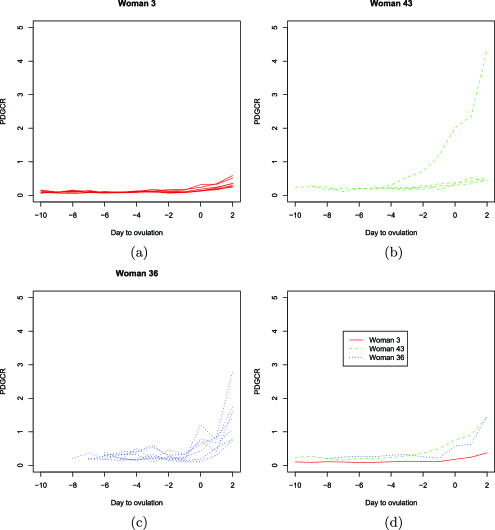
Figure 1: Comparison of hormone profiles for three women in the Early Pregnancy Study. Frames (a) to (c) show multiple profiles for each woman, while frame (d) shows the average profile for each woman.

In order to provide some insight into the challenges associated with functional clustering in the context of the EPS, consider the hormonal profiles depicted in Figure 1. Frames (a) to (c) depict the hormone profiles for 3 women, while frame (d) shows the mean profile corresponding to each one of them, obtained by simply averaging all available observations at a given day within the cycle. When looking at the mean profiles in (d), women 43 and 36 seem to have very similar hormonal responses, which are different from those of woman 3. However, when the individual profiles are considered, it is clear that most of the cycles of woman 43 look like those of woman 3 and that the big difference in the means is driven by the single abnormal cycle. This result, although not surprising if we consider that means are notoriously nonrobust, suggests that simple approaches that average profiles over individuals (or, equivalently, use Gaussian distributions to describe subject-specific variability) might not be the most appropriate for this type of data.

The use of Bayesian nonparametric mixture models for clustering has a long history [Medvedovic and Sivaganesan (2002), Quintana and Iglesias (2003), Lau and Green (2007)] and presents a number of practical advantages over other model-based clustering techniques. Nonparametric mixtures induce a probability distribution on the space of partitions of the data, therefore, we do not need to specify in advance the number of clusters in the sample. Once updated using the data, this distribution on partitions allows us to assess variability, and hence characterize uncertainty in the clustering structure (including that associated with the estimation of the curves), providing a more complete picture than classical methods. In this paper, we work with a generalized Dirichlet process (GDP) first introduced by Hjort (2000) and study some of its properties as a clustering tool. In particular, we show that the GDP generates a richer prior on data partitions than those induced by popular models such as the Dirichlet process [Ferguson (1973)] or the two-parameter Poisson–Dirichlet process [Pitman (1996)], as it allows for an asymptotically bounded number of clusters in addition to logarithmic and power-law rates of growth.

The paper is organized as follows: Section 2 reviews the basics of nonparametric regression and functional clustering, while Section 3 explores the design of nonparametric mixture models for functional clustering. Building on these brief reviews, Section 4 describes two Bayesian approaches to functional clustering in nested designs, while Section 5 describes Markov chain Monte Carlo algorithms for this problem. An illustration focused on the EPS is presented in Section 6. Finally, Section 7 presents a brief discussion and future research directions.

2 Model-based functional clustering

To introduce our notation, consider first a simple functional clustering problem where multiple noisy observations are collected from functions $f_{1},\ldots,f_{I}$. More specifically, for subjects $i=1,\ldots,I$ and within-subject design points $t=1,\ldots,T_{i}$, observations consist of ordered pairs $(x_{it},y_{it})$, where

$$y_{it} = f_{i}(x_{it})+\varepsilon_{it},\qquad\varepsilon_{it}\sim\mathsf{N}\bigl{(}0,\sigma_{i}^{2}\bigr{)}.$$

For example, in the EPS, $y_{it}$ corresponds to the level of progesterone in the blood of woman $i$ collected at day $x_{it}$ of the menstrual cycle, and $f_{i}$ denotes a smooth trajectory in progesterone for woman $i$ (initially supposing a single menstrual cycle of data from each woman), and clusters in $\{f_{i}\}_{i=1}^{I}$ could provide insight into the variability in progesterone curves across women, while potentially allowing us to identify abnormal or outlying curves.

If all curves are observed at the same covariate levels (i.e., $T_{i}=T$ and $x_{it}=x_{t}$ for every $i$), a natural approach to functional clustering is to apply standard clustering methods to the data vectors, ${\mathbf{y}}_{i}=(y_{i1},\ldots,y_{iT})^{\prime}$. For example, in the spirit of Ramsay and Silverman (2005), one could apply hierarchical or $k$-means clustering to the first few principal components [Yeung and Ruzzo (2001)]. Alternatively, with uneven spacings or missing observations, nonparametric regression techniques such as kernel regression [e.g., see Li and Racine (2004), Racine and Li (2004)] could be used to interpolate the value of the curves to a common grid, and then traditional clustering techniques could be applied. From a model-based perspective, one could instead suppose that ${\mathbf{y}}_{i}$ is drawn from a mixture of $k$ multivariate Gaussian distributions, with each Gaussian corresponding to a different cluster [Fraley and Raftery (2002), Yeung et al. (2001)]. The number of clusters could then be selected using the BIC criteria [Fraley and Raftery (2002), Li (2005)] or a nonparametric Bayes approach could be used to bypass the need for this selection, while allowing the number of clusters represented in a sample of $I$ individuals to increase stochastically with sample size [Medvedovic and Sivaganesan (2002)].

A more general approach that allows us to deal with unevenly spaced and missing observations is to fit a nonparametric model to each curve and then project all the curves onto a common space. For example, we can represent the unknown function $f_{i}$ as a linear combination of prespecified basis functions $\{b_{k}\}_{k=1}^{p}$, that is, we can write

$$f_{i}(x_{it}) = \theta_{i0}+\sum_{k=1}^{p}\theta_{ik}b_{k}(x_{it}),$$

where $\bolds{\theta}_{i}=(\theta_{i0},\theta_{i1},\ldots,\theta_{ip})$ are basis coefficients specific to subject $i$, with variability in these coefficients controlling variability in the curves $\{f_{i}\}_{i=1}^{I}$. A common approach to functional clustering is to induce clustering of the curves through clustering of the basis coefficients [Abraham et al. (2003), Heard, Holmes and Stephens (2006)]. Then the methods discussed above for clustering of the data vectors $\{{\mathbf{y}}_{i}\}_{i=1}^{I}$ in the balanced design case can essentially be applied directly to the basis coefficients $\{\bolds{\theta}_{i}\}_{i=1}^{I}$.

Although the methods apply directly to other choices of basis functions, our focus will be on splines, which have been previously used in the context of hormone profiles [Brumback and Rice (1998), Bigelow and Dunson (2009)]; given a set of knots $\tau_{1},\ldots,\tau_{p}$, the $k$th member of the basis system is defined as

$$b_{k}(x) = (x-\tau_{k})_{+}^{q},$$

where $(\cdot)_{+}=\max\{\cdot,0\}$. Given the knot locations, inferences on $\bolds{\theta}_{i}$ and $\sigma^{2}_{i}$ can be carried out using standard linear regression tools, however, selecting the number and location of the nodes $\tau_{1},\ldots,\tau_{p}$ can be a challenging task. A simple solution is to use a large number of equally spaced knots, together with a penalty term on the coefficients to prevent overfitting. From a Bayesian perspective, this penalty term can be interpreted as a prior on the spline coefficients; for example, the maximum likelihood estimator (MLE) obtained under an $L^{2}$ penalty on the spline coefficients is equivalent to the maximum a posteriori estimates for a Bayesian model under a normal prior, while the MLE under an $L^{1}$ penalty is equivalent to the maximum a posterior estimate under independent double-exponential priors on the spline coefficients.

Instead of the more traditional Gaussian and double exponential priors, in this paper we focus on zero-inflated priors, in the spirit of Smith and Kohn (1996). Priors of this type enforce sparsity by zeroing out some of the spline coefficients and, by allowing us to select a subset of the knots, provides adaptive smoothing. In their simpler form, zero-inflated priors assume that the coefficients are independent from each other and that

$$\theta_{ik}|\gamma,\sigma^{2}_{i} \sim \gamma\mathsf{N}\bigl{(}0,\omega_{k}\sigma_{i}^{2}\bigr{)}+(1-\gamma)\delta_{0},\qquad\sigma_{i}^{2}\sim\mathsf{IGam}(\nu_{1},\nu_{2}),$$ (1)

where $\delta_{x}$ denotes the degenerate distribution putting all its mass at $x$, $\omega_{k}$ controls the overdispersion of the coefficients with respect to the observations and $\gamma$ is the prior probability that the coefficient $\theta_{ik}$ is different from zero. In order to incorporate a priori dependence across coefficients, we can reformulate the hierarchical model by introducing Bernoulli random variables $\lambda_{i1},\ldots,\lambda_{ip}$ such that

$$\mathbf{y}_{i}|\bolds{\theta}_{i},\sigma^{2}_{i},\bolds{\Lambda}_{i} \sim \mathsf{N}\bigl{(}\mathbf{B}(\mathbf{x}_{i})\bolds{\Lambda}_{i}\bolds{\theta}_{i},\sigma^{2}_{i}\mathbf{I}\bigr{)},\qquad\bolds{\theta}_{i}|\sigma_{i}^{2}\sim\mathsf{N}\bigl{(}\mathbf{0},\sigma_{i}^{2}\bolds{\Omega}\bigr{)},$$

$$\sigma_{i}^{2} \sim \mathsf{IGam}(\nu_{1},\nu_{2}),$$

where $\mathbf{y}_{i}=(y_{i1},\ldots,y_{iT_{i}})$ and $\mathbf{x}_{i}=(x_{i1},\ldots,x_{iT_{i}})$ are, respectively, the vectors of responses and covariates associated with subject $i$, $\mathbf{B}(\mathbf{x}_{i})$ is the matrix of basis functions also associated with subject $i$ with entries $[\mathbf{B}(\mathbf{x}_{i})]_{tk}=b_{k}(x_{it})$, $\bolds{\Lambda}_{i}=\operatorname{diag}\{\lambda_{i1},\ldots,\lambda_{ip}\}$ and $\lambda_{i}$ equals 1 independently with probability $\gamma$, and $\bolds{\Omega}$ is a $p\times p$ covariance matrix. Note that if $\bolds{\Omega}$ is a diagonal matrix and $[\bolds{\Omega}]_{kk}=\omega_{k}$, we recover the independent priors in (1). For the single curve case, choices for $\bolds{\Omega}$ based on the regression matrix $\mathbf{B}(\mathbf{x}_{i})$ are discussed in DiMatteo, Genovese and Kass (2001), Liang et al. (2008) and Paciorek (2006).

Although the preceding two-stage approach is simple to implement using off-the-shelf software, it ignores the uncertainty associated with the estimation of the basis coefficients while clustering the curves. In the spirit of Fraley and Raftery (2002), an alternative that deals with this issue is to employ a mixture model of the form

$$\mathbf{y}_{i}|\bigl{\{}\bolds{\theta}^{*}_{k}\bigr{\}},\bigl{\{}\sigma^{*2}_{k}\bigr{\}},\bigl{\{}\bolds{\Lambda}^{*}_{k}\bigr{\}} \sim \sum_{k=1}^{K}w_{k}\mathsf{N}\bigl{(}\mathbf{B}(\mathbf{x}_{j})\bolds{\Lambda}^{*}_{k}\bolds{\theta}^{*}_{k},\sigma^{*2}_{k}\mathbf{I}\bigr{)},\qquad\sum_{k=1}^{K}w_{k}=1,$$ (2)

where $\bolds{\theta}^{*}_{k}$ is the vector of coefficients associated with the $k$th cluster, $\bolds{\Lambda}^{*}_{k}$ is the diagonal selection matrix for the $k$th cluster, $\sigma_{k}^{*2}$ is the observational variance associated with observations collected in the $k$th cluster, $w_{k}$ can be interpreted as the proportion of curves associated with cluster $k$, and $K$ is the maximum number of clusters in the sample. From a frequentist perspective, estimation of this model can be performed using expectation–maximization (EM) algorithms, while selection of the number of mixture components can be carried out using the BIC. Alternatively, Bayesian inference can be performed for this model using Markov chain Monte Carlo (MCMC) algorithms once appropriate priors for the vector $\mathbf{w}=(w_{1},\ldots,w_{K})$ and the cluster-specific parameters $(\bolds{\theta}^{*}_{k},\bolds{\Lambda}_{k}^{*},\sigma_{k}^{*2})$ have been chosen, opening the door to simple procedures for the estimation of the number of clusters in the sample.

3 Bayesian nonparametric mixture models for functional data

Note that the model in (2) can be rewritten as a hierarchical model by introducing latent variables $\{(\bolds{\theta}_{i},\sigma_{i}^{2},\bolds{\Lambda}_{i})\}_{i=1}^{I}$ so that

$$\mathbf{y}_{i}|\bolds{\theta}_{i},\sigma^{2}_{i},\bolds{\Lambda}_{i} \sim \mathsf{N}\bigl{(}\mathbf{B}(\mathbf{x}_{i})\bolds{\Lambda}_{i}\bolds{\theta}_{i},\sigma^{2}_{i}\mathbf{I}\bigr{)},\qquad\bolds{\theta}_{i},\sigma^{2}_{i},\bolds{\Lambda}_{i}|G\sim G,$$

$$G(\cdot) = \sum_{k=1}^{K}w_{k}\delta_{(\bolds{\theta}^{*}_{k},\sigma^{*2}_{k},\bolds{\Lambda}_{k}^{*})}(\cdot).$$

Therefore, specifying a joint prior on $\mathbf{w}$ and $\{(\bolds{\theta}^{*}_{k},\sigma_{k}^{*2},\bolds{\Lambda}^{*}_{k})\}_{k=1}^{K}$ is equivalent to specifying a prior on the discrete distribution $G$ generating the latent variables $\{(\bolds{\theta}_{i},\sigma_{i}^{2},\bolds{\Lambda}_{i})\}_{i=1}^{I}$. In this section we discuss strategies to specify a flexible prior distribution on this mixing distribution in the context of functional clustering. In particular, we concentrate on nonparametric specifications for $G$ through the class of stick-breaking distributions.

A stick-breaking prior [Ishwaran and James (2001), Ongaro and Cattaneo (2004)] with baseline measure $G_{0}$ and precision parameters $\{a_{l}\}_{l=1}^{L}$ and $\{b_{l}\}_{l=1}^{L}$ is defined as

$$G(\cdot) = \sum_{k=1}^{K}w_{k}\delta_{\bolds{\vartheta}_{k}}(\cdot),$$ (4)

where the atoms $\{\bolds{\vartheta}_{k}\}_{k=1}^{K}$ are independent and identically distributed samples from $G_{0}$ and the weights $\{w_{k}\}_{l=1}^{K}$ are constructed as $w_{k}=u_{k}\prod_{s<k}(1-u_{s})$, with $\{u_{k}\}_{k=1}^{K}$ another independent and identically distributed sequence of random variables such that $u_{k}\sim\mathsf{Beta}(a_{k},b_{k})$ for $k<K$ and $u_{K}=1$. For example, taking $K=\infty$, $a_{k}=1-a$ and $b_{k}=b+ka$ for $0\leq a<1$ and $b>-a$ yields the two-parameter Poisson–Dirichlet process [Pitman (1995), Ishwaran and James (2001)], denoted $\mathsf{PY}(a,b,G_{0})$, with the choice $a=0$ resulting in the Dirichlet process [Ferguson (1973), Sethuraman (1994)], denoted $\mathsf{DP}(b,G_{0})$. In mixture models such as (3), $G_{0}$ acts as the common prior for the cluster-specific parameters $\{\bolds{\vartheta}_{k}\}_{k=1}^{K}$, while the sequences $\{a_{k}\}_{k=1}^{K}$ and $\{b_{k}\}_{k=1}^{K}$ control the a priori expected number and size of the clusters.

The main advantage of nonparametric mixture models such as the Poisson–Dirichlet process as a clustering tool is that they allow for automatic inferences on the number of components in the mixture. Indeed, these models induce a prior probability on all possible partitions of the set of observations, which is updated based on the information contained in the data. However, Poisson–Dirichlet processes have two properties that might be unappealing in our EPS application; first, they place a relatively large probability on partitions that include many small clusters and, second, they imply that the number of clusters will tend to grow logarithmically (if $a=0$) or as a power law (if $a>0$) as more observations are included in the data set. However, priors that favor Introduction of increasing numbers of clusters without bound as the number of subjects increase have some disadvantages in terms of interpretability and sparsity in characterizing high-dimensional data. For example, in applying DP mixture models for clustering of the progesterone curves in EPS, Bigelow and Dunson (2009) obtained approximately 32 different clusters, with half of these clusters singletons. Many of the clusters appeared similar, and it may be that this large number of clusters was partly an artifact of the DP prior. Dunson (2009) proposed a local partition process prior to reduce dimensionality in characterizing the curves, but this method does not produce easily interpretable functional clusters. Hence, it is appealing to use a more flexible global clustering prior that allows the number of clusters to instead converge to a finite constant.

With this motivation, we focus on the generalized Dirichlet process (GDP) introduced by Hjort (2000), denoted $\mathsf{GDP}(a,b,G_{0})$. The GDP corresponds to a stick-breaking prior with $K=\infty$, $a_{k}=a$ and $b_{k}=b$ for all $k$. When compared against the Poisson–Dirichlet process, the GDP has quite distinct properties.

Theorem 1

Let $Z_{n}$ be the number of distinct observations in a sample of size $n$ from a distribution $G$, where $G\sim\mathsf{GDP}(a,b,G_{0})$. The expected number of clusters $\mathsf{E}(Z_{n})$ is given by

$$\mathsf{E}(Z_{n}) = \sum_{i=1}^{n}\frac{ia\Gamma(a+b)\Gamma(b+i-1)}{\Gamma(b)\Gamma(a+b+i)-\Gamma(a+b)\Gamma(b+i)}.$$ (5)

The proof can be seen in Appendix A. Note that for $a=1$, this expression simplifies to $\mathsf{E}(Z_{n})=\sum_{i=1}^{n}\frac{b}{b+i-1}\sim o(\log n)$, a well-known result for the Dirichlet process [Antoniak (1974)]. Letting $W_{n}=Z_{n}-Z_{n-1}$ denote the change in the number of clusters in adding the $n$th individual to a sample with $n-1$ subjects, Stirling’s approximation can be used to show that

$$\mathsf{E}(W_{n})=\frac{na\Gamma(a+b)\Gamma(b+n-1)}{\Gamma(b)\Gamma(a+b+n)-\Gamma(a+b)\Gamma(b+n)}\approx C(a,b)n^{-a},$$

where $C(a,b)=\{a\Gamma(a+b)/\Gamma(b)\}\exp\{-2(a+1)\}$. Hence, $\mathsf{E}(W_{n})\to 0$ as $n\to\infty$ and new clusters become increasingly rare as the sample size increases. Note that for $a\leq 1$, the number of clusters will grow slowly but without bound as $n$ increases, with $\mathsf{E}(Z_{n})\to\infty$. The rate of growth in this case is proportional to $n^{1-a}$, which is similar to what is obtained by using the Poisson Dirichlet prior [Sudderth and Jordan (2009)]. However, when $a>1$ the expected number of clusters instead converges to a finite constant, which is a remarkable difference compared with the Dirichlet and Poisson–Dirichlet process. As mentioned above, there may be a number of practical advantages to bounding the number of clusters. In addition, a finite bound on the number clusters seems to be more realistic in many applications, including the original species sampling applications that motivated much of the early development in this area [McCloskey (1965), Pitman (1995)].

In order to gain further insight into the clustering structure induced by the $\mathsf{GDP}(a,b,G_{0})$, we present in Figure 2 the relationship between the size of the largest cluster and the mean number of clusters in the partition (left panel), and the mean cluster size and the number of clusters (right panel) for a sample of size $n=1000$. The numbers presented in this figure are based on the results from 20,000 simulations from the stick-breaking prior. Each continuous line corresponds to a combination of shape parameters such that $a/(a+b)$ is constant, while the dashed line in the plots corresponds to the combinations available under a Dirichlet process. The plots demonstrate that the additional parameter in the GDP allows us to simultaneously control the number of clusters and the relative size of the clusters, increasing the flexibility of the model as a clustering procedure.

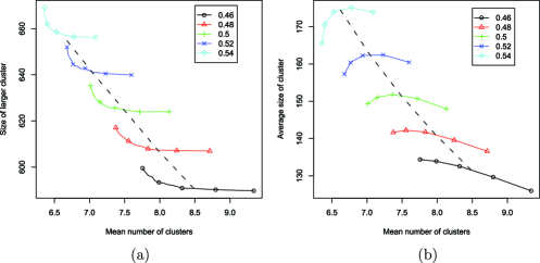
Figure 2: Clustering structure induced by a $\mathsf{GDP}(a,b,G_{0})$ for a sample of size $n=1000$. Panel (a) shows the relationship between the size of the largest cluster and the mean number of clusters for different GDPs, where each curve shares a common $\mathsf{E}(u_{k})=a/(a+b)$. Panel (b) shows the relationship between the average cluster size and the mean number of clusters. The dashed lines correspond to the combinations available under a standard Dirichlet process.

The previous discussion focused on the impact of the prior distribution for the mixture weights on the clustering structure. Another important issue in the specification of the model is the selection of the baseline measure $G_{0}$. Note that in the functional clustering setting $\bolds{\vartheta}_{k}=(\bolds{\theta}^{*}_{k},\sigma_{k}^{*2},\bolds{\Lambda}^{*}_{k})$ and, therefore, a computationally convenient choice that is in line with our previous discussion on basis selection and zero-inflated priors is to write

$$G_{0}\bigl{(}\bolds{\theta},\sigma^{2},\bolds{\Lambda}\bigr{)} = \mathsf{N}\bigl{(}\bolds{\theta}|\mathbf{0},\sigma^{2}\bolds{\Omega}\bigr{)}\times\mathsf{IGam}\bigl{(}\sigma^{2}|\nu_{1},\nu_{2}\bigr{)}\times\prod_{s=1}^{p}\mathsf{Ber}(\lambda_{s}|\gamma).$$ (6)

A prior of this form allows differential adaptive smoothing for each cluster in the data; the level of smoothness is controlled by $\gamma$ (the prior probability of inclusion for each of the spline coefficients) and, therefore, it is convenient to assign to it a hyperprior such as $\gamma\sim\mathsf{Beta}(\eta_{1},\eta_{2})$.

4 Functional clustering in nested designs

Consider now the case where multiple curves are collected for each subject in the study. In this case, the observations consist of ordered pairs $(y_{ijt},x_{ijt})$ where

$$y_{ijt} = f_{ij}(x_{ijt})+\varepsilon_{ijt},$$

where $f_{ij}$ is the $j$th functional replicate for subject $i$, with $i=1,\ldots,I$, $j=1,\ldots,n_{i}$ and $t=1,\ldots,T_{ij}$. For example, in the EPS, $f_{ij}$ is the measurement error-corrected smooth trajectory in the progesterone metabolite PdG over the $j$th menstrual cycle from woman $i$, with $t$ indexing the sample number and $x_{ijt}$ denoting the day within the $i,j$ menstrual cycle relative to a marker of ovulation day.

A natural extension of (3) to nested designs arises by modeling the expected evolution of progesterone in time for cycle $j$ of woman $i$ as $f_{ij}=\mathbf{B}(\mathbf{x}_{ij})\bolds{\theta}_{ij}$ and using a hierarchical model for the set of curve-specific parameters $\{\bolds{\theta}_{ij}\}$ in order to borrow information across subjects and/or replicates. In the following subsections, we introduce two alternative nonparametric hierarchical priors that avoid parametric assumptions on the distribution of the basis coefficients, while inducing hierarchical functional clustering.

4.1 Mean-curve clustering

As a first approach, we consider a Gaussian mixture model, which characterizes the basis coefficients for functional replicate $j$ from subject $i$ as conditionally independent draws from a Gaussian distribution with subject-specific mean and variance, in the spirit of Booth, Casella and Hobert (2008):

$$\mathbf{y}_{ij}|\bolds{\theta}_{ij},\sigma_{i} \sim \mathsf{N}\bigl{(}\mathbf{B}(\mathbf{x}_{ij})\bolds{\theta}_{ij},\sigma_{i}^{2}\mathbf{I}\bigr{)},\qquad\bolds{\theta}_{ij}|\bolds{\theta}_{i},\bolds{\Lambda}_{i},\sigma^{2}_{i}\sim G_{i},$$

$$G_{i} = \mathsf{N}\bigl{(}\bolds{\Lambda}_{i}\bolds{\theta}_{i},\sigma^{2}_{i}\bolds{\Sigma}\bigr{)},$$

where $\bolds{\Lambda}_{i},\bolds{\theta}_{i},\sigma_{i}^{2}$ are as described in expression (3) and $\bolds{\Sigma}$ is a $p\times p$ covariance matrix. In this model, the average curve for subject $i$ is obtained as $\mathsf{E}\{f_{ij}(x)|\bolds{\Lambda}_{i},\bolds{\theta}_{i},\sigma_{i}^{2}\}={\mathbf{B}}(x)\bolds{\Lambda}_{i}\bolds{\theta}_{i}$, with $\bolds{\Lambda}_{i}$ providing a mechanism for subject-specific basis selection, so that the curves from subject $i$ only depend on the basis functions corresponding to nonzero diagonal elements of $\bolds{\Lambda}_{i}$. The variability in the replicate curves for the same subject is controlled by $\sigma_{i}^{2}\bolds{\Sigma}$, with the subject-specific multiplier allowing subjects to vary in the degree of variability across the replicates. The need to allow such variability is well justified in the hormone curve application.

In order to borrow information across women, we need a hyperprior for the woman specific parameters $\{(\bolds{\Lambda}_{i},\sigma_{i}^{2},\bolds{\theta}_{i})\}_{i=1}^{I}$. Since we are interested in clustering subjects, a natural approach is to specify this hyperprior nonparametrically through a generalized Dirichlet process centered around the baseline measure in (6), just as we did for the single curve case. This yields

$$\bigl{(}\bolds{\theta}_{i},\sigma_{i}^{2},\bolds{\Lambda}_{i}\bigr{)}|G \sim G,\qquad G\sim\mathsf{GDP}(a,b,G_{0})$$

with $G_{0}$ given in (6). Since the distribution $G$ is almost surely discrete, the model identifies clusters of women with similar average curves. This is clearer if we integrate the curve-specific coefficients $\{\bolds{\theta}_{ij}\}$ and the unknown distribution $G$ out of the model to obtain

$$\mathbf{y}_{i1},\ldots,\mathbf{y}_{in_{i}}|\{w_{k}\},\bigl{\{}\bolds{\theta}_{k}^{*}\bigr{\}},\bigl{\{}\sigma_{k}^{*2}\bigr{\}},\bigl{\{}\bolds{\Lambda}_{k}^{*}\bigr{\}}$$

(8)

$$\qquad\sim\sum_{k=1}^{K}w_{k}\Biggl{\{}\prod_{j=1}^{n_{i}}\mathsf{N}\bigl{(}\mathbf{B}(\mathbf{x}_{ij})\bolds{\Lambda}_{k}^{*}\bolds{\theta}_{k}^{*},\sigma^{*2}_{k}(\mathbf{I}+\bolds{\Sigma})\bigr{)}\Biggr{\}}.$$

By incorporating the distribution of the selection matrices $\bolds{\Lambda}_{1},\ldots,\bolds{\Lambda}_{I}$ in the random distribution $G$, this model allows for a different smoothing pattern for each cluster of curves. This is an important difference with a straight generalization of the model in Ray and Mallick (2006), who instead treat the selection matrix as a hyperparameter in the baseline measure $G_{0}$ and therefore induce a common smoothing pattern across all clusters.

The model is completed by assigning priors for the hyperparameters. For the random effect variances we take inverse-Wishart priors:

$$\bolds{\Omega} \sim \mathsf{IWis}(\nu_{\Omega},\bolds{\Omega}_{0}),\qquad\bolds{\Sigma}\sim\mathsf{IWis}(\nu_{\Sigma},\bolds{\Sigma}_{0}).$$

In the spirit of the unit information priors [Paciorek (2006)], the hyperparameters for these priors can be chosen so that $\bolds{\Omega}_{0}$ and $\bolds{\Sigma}_{0}$ are proportional to

$$\sum_{i=1}^{I}\sum_{j=1}^{n_{i}}\mathbf{B}(\mathbf{x}_{ij})^{\prime}\mathbf{B}(\mathbf{x}_{ij}).$$

Finally, the concentration parameters $a$ and $b$ are given gamma priors $a\sim\mathsf{Gam}(\kappa_{a},\tau_{a})$ and $b\sim\mathsf{Gam}(\kappa_{b},\tau_{b})$ and the probability of inclusion $\gamma$ is assigned a beta prior, $\gamma\sim\mathsf{Beta}(\eta_{1},\eta_{2})$.

4.2 Distribution-based clustering

Because the subject-specific distributions $\{G_{i}\}_{i=1}^{I}$ were assumed to be Gaussian and the nonparametric prior was placed on their means, the model in the previous section clusters subjects based on their average profile. However, as we discussed in Section 1, clustering based on the mean profiles might be misleading in studies such as the EPS in which there are important differences among subjects in not only the mean curve but also the distribution about the mean. In hormone curve applications, it is useful to identify clusters of trajectories over the menstrual cycle to study variability in the curves and identify outlying cycles that may have reproductive dysfunction. It is also useful to cluster women based not simply on the average curve but on the distribution of curves. With this motivation in mind, we generalize our hierarchical nonparametric specification to construct a model with additional parameters that enables clustering based on more than proximity between the mean curves. This generalization further enables clustering within subjects as well as subjects.

To motivate our nonparametric construction, consider first the simpler case in which there are only two types of curves in each cluster of women (say, normal and abnormal), so that it is natural to model the subject-specific distribution as a two-component mixture where

$$\mathbf{y}_{ij}|\varpi_{i},{\bolds{\Lambda}}_{1i},{\bolds{\theta}}_{1i},{\sigma}^{2}_{1i},{\bolds{\Lambda}}_{2i},{\bolds{\theta}}_{2i},{\sigma}^{2}_{2i}$$

(9)

$$\qquad\sim\varpi_{i}\mathsf{N}\bigl{(}\mathbf{B}(\mathbf{x}_{ij}){\bolds{\Lambda}}_{1i}{\bolds{\theta}}_{1i},{\sigma}^{2}_{1i}\mathbf{I}\bigr{)}+(1-\varpi_{i})\mathsf{N}\bigl{(}\mathbf{B}(\mathbf{x}_{ij}){\bolds{\Lambda}}_{2i}{\bolds{\theta}}_{2i},{\sigma}^{2}_{2i}\mathbf{I}\bigr{)},$$

$\varpi_{i}$ can be interpreted as the proportion of curves from subject $i$ that are in group 1 (say, normal), and $({\bolds{\theta}}_{1i},{\sigma}^{2}_{1i})$ are the parameters that describe curves from a normal cycle, ${\bolds{\Lambda}}_{1i}$ is a diagonal variable selection matrix for the normal cycles that zeroes out unnecessary coefficients to avoid overfitting, $({\bolds{\theta}}_{2i},{\sigma}^{2}_{2i})$ are the parameters describing the curves from an abnormal cycle, and ${\bolds{\Lambda}}_{2i}$ is the variable selection matrix for the abnormal cycles. Note that in this case we have not one but two variance parameters for each individual, which provide additional flexibility by allowing each cluster of curves to present a different level of observational noise. This feature is desirable in the EPS because, for a given woman, observational noise in abnormal cycles tends to be larger than in normal cycles.

Under this formulation, the subject-specific distribution is described by the vector of parameters $(\varpi_{i},{\bolds{\Lambda}}_{1i},{\bolds{\theta}}_{1i},{\sigma}^{2}_{1i},{\bolds{\Lambda}}_{2i},{\bolds{\theta}}_{2i},{\sigma}^{2}_{2i})$, and clustering subjects could be accomplished by clustering these vectors. We can accomplish this by using another mixture model that mimics (2) and (4.1), so that

$$\mathbf{y}_{i1},\ldots,\mathbf{y}_{in_{i}}|\{\pi_{k}\},\{\varpi_{k}\},\bigl{\{}\bolds{\theta}^{*}_{1k}\bigr{\}},\bigl{\{}\sigma_{1k}^{*2}\bigr{\}},\bigl{\{}\bolds{\Lambda}_{1k}^{*}\bigr{\}},\bigl{\{}\bolds{\theta}^{*}_{2k}\bigr{\}},\bigl{\{}\sigma_{2k}^{*2}\bigr{\}},\bigl{\{}\bolds{\Lambda}_{2k}^{*}\bigr{\}}$$

$$\qquad\sim\sum_{k=1}^{K}\pi_{k}\prod_{j=1}^{n_{i}}\bigl{\{}\varpi_{k}\mathsf{N}\bigl{(}\mathbf{B}(\mathbf{x}_{ij}){\bolds{\Lambda}}^{*}_{1k}{\bolds{\theta}}^{*}_{1k},{\sigma}^{*2}_{1k}\mathbf{I}\bigr{)}$$ (10)

$$\hskip 80.0pt{}+(1-\varpi_{k})\mathsf{N}\bigl{(}\mathbf{B}(\mathbf{x}_{ij}){\bolds{\Lambda}}^{*}_{2l}{\bolds{\theta}}^{*}_{2k},{\sigma}^{*2}_{1k}\mathbf{I}\bigr{)}\bigr{\}}.$$

To formulate our Bayesian nonparametric model for clustering, we start by rewriting (4.2) as a general mixture model where

$$\mathbf{y}_{ij}|\bolds{\theta}_{ij},\sigma^{2}_{ij},\bolds{\Lambda}_{ij} \sim \mathsf{N}\bigl{(}\mathbf{B}(\mathbf{x}_{ij})\bolds{\Lambda}_{ij}\bolds{\theta}_{ij},\sigma^{2}_{ij}\mathbf{I}\bigr{)},\qquad\bolds{\theta}_{ij},\sigma^{2}_{ij},\bolds{\Lambda}_{ij}|G_{i}\sim G_{i}$$ (11)

and $G_{i}$ is a discrete distribution which is assigned a nonparametric prior. Note that this is analogous to the formulation in (4.1), but by replacing the Gaussian distribution with a random distribution with a nonparametric prior we are modeling the within-subject variability by clustering curves into groups with homogeneous shape.

Now, we need to define a prior over the collection $\{G_{i}\}_{i=1}^{I}$ that induces clustering among the distributions. For example, we could use a discrete distribution whose atoms are in turn random distributions, for example,

$$G_{i} \sim \sum_{k=1}^{\infty}\pi_{k}\delta_{G_{k}^{*}},$$

where $\pi_{k}=v_{k}\prod_{s<k}(1-v_{s})$, $v_{k}\sim\mathsf{Beta}(a_{1},b_{1})$ and $G_{k}^{*}\sim\mathsf{GDP}(a_{2},b_{2},G_{0})$ independently. This implies that

$$G_{k}^{*} = \sum_{l=1}^{\infty}\varpi_{lk}\delta_{(\bolds{\theta}_{lk}^{*},\sigma_{lk}^{2*},\bolds{\Lambda}_{lk}^{*})},\qquad\bigl{(}\bolds{\theta}_{lk}^{*},\sigma_{lk}^{2*},\bolds{\Lambda}_{lk}^{*}\bigr{)}\sim G_{0},$$

with $\varpi_{lk}=u_{lk}\prod_{s<l}(1-u_{sk})$ and $u_{lk}\sim\mathsf{Beta}(a_{2},b_{2})$ and $G_{0}$ as in (6). Therefore, if we were to replace the collection $\{G^{*}_{k}\}_{k=1}^{\infty}$ with random discrete distributions with only two atoms and we were to integrate over the random distributions $\{G_{i}\}_{i=1}^{I}$, this model would be equivalent to (4.2) with $K=\infty$.

This model on the collection $\{G_{i}\}_{i=1}^{I}$ is a generalization of the nested Dirichlet process introduced in Rodríguez, Dunson and Gelfand (2008) and, as with other models based on nested nonparametric processes, interesting special cases can be obtained by considering the limit of the precision parameters. For example, letting $b_{2}\to 0$ while keeping $a_{2}$ fixed induces a model where all menstrual cycles within a woman are assumed to have the same profile, and subjects are clustered according to their mean cycle. Such a model is equivalent to the one obtained by taking $\bolds{\Sigma}\to 0$ in (4.1). On the other hand, by letting $b_{1}\to\infty$ while keeping $a_{1}$ constant, we obtain a model where all subjects are treated as different and menstrual cycles are clustered within each women. In this case, information is borrowed across the menstrual cycles of each women, but not across women.

Intuitively, we can think of the model we just described as first clustering curves within a subject via a model-based version of $k$-means applied to the subject-specific basis coefficients. Then, two subjects having similar distributions of curve clusters will be clustered together. Because we use a joint hierarchical model, these stages are done simultaneously.

Again, the model is completed by specifying prior distributions on the remaining parameters. As before, we let $\bolds{\Omega}\sim\mathsf{IWis}(\nu_{\Omega},\bolds{\Omega}_{0})$, $\nu_{2}\sim\mathsf{Gam}(\rho,\psi)$ and $\gamma\sim\mathsf{Beta}(\eta_{1},\eta_{2})$, providing a conditionally conjugate specification amenable for simple computational implementation. Finally, for the precision priors of the GDPs we set

$$a_{1} \sim \mathsf{Gam}(\kappa_{a_{1}},\tau_{a_{1}}),\qquad b_{1}\sim\mathsf{Gam}(\kappa_{b_{1}},\tau_{b_{1}}),$$

$$a_{2} \sim \mathsf{Gam}(\kappa_{a_{2}},\tau_{a_{2}}),\qquad b_{2}\sim\mathsf{Gam}(\kappa_{b_{2}},\tau_{b_{2}}).$$

5 Computation

As is commonplace in Bayesian inference, we resort to Markov chain Monte Carlo (MCMC) algorithms [Robert and Casella (1999)] for computation in our functional clustering models. Given an initial guess for all unknown parameters in the model, the algorithms proceed by sequentially sampling blocks of parameters from their full conditional distributions. In particular, we design our algorithms using truncated versions of the GDP and the nested GDP, where a large but finite number of atoms are used to approximate the nonparametric mixture distributions. Well-known results on the convergence of truncations as the number of atoms grows that were originally presented in Ishwaran and James (2001) and Rodríguez, Dunson and Gelfand (2008) can be directly extended to this problem (see Appendix B). Furthermore, because most components of the model are conditionally conjugate, most of the full conditional distributions can be directly sampled using Gibbs steps. Full details of the algorithm can be seen in the online supplementary materials [Rodriguez and Dunson (2014)].

Convergence of the MCMC algorithms was assessed using the multi-chain method described in Gelman and Rubin (1992), which was applied to monitor the (unnormalized) posterior distribution, as well as the number of occupied clusters on each level of the model and the Frobenius norm of the matrices $\bolds{\Omega}$ and $\bolds{\Sigma}$.

6 The Early Pregnancy Study

Progesterone plays a crucial role in controlling different aspects of reproductive function in women, from fertilization to early development and implantation. Therefore, understanding the variability of hormonal profiles across the menstrual cycle and across subjects is important in understanding mechanisms of infertility and early pregnancy loss, as well as for developing approaches for identifying abnormal menstrual cycles and women for diagnostic purposes. Our data, extracted from the Early Pregnancy Study [Wilcox et al. (1998)], consists of log daily creatinine-corrected concentrations of pregnanediol-3-glucuronide (PdG) for 60 women along multiple menstrual cycles, measured in micrograms per milligram of creatinine (µg$/$ml Cr). We focus on 13-day intervals extending from 10 days before ovulation to 2 days after ovulation. According to the results in Dunson et al. (1999), this interval should include the fertile window of the menstrual cycle during which noncontracepting intercourse has a nonneglible probability of resulting in a conception. Also, for this illustration we considered only nonconceptive cycles and women with at least four cycles in each record. Therefore, the number of curves per woman varies between 4 and 9.

We analyzed the EPS data using both the mean-based clustering model described in Section 4.1 and the distribution-based clustering model of Section 4.2. These models where fitted using the algorithms from Section 5. In the mean-based clustering algorithm, the GDP was truncated so that $K=40$, while in the distribution-based algorithm the nested GDP was truncated so that $K=40$ and $L=30$. Although these numbers might seem large given the sample sizes involved, a large number of empty components are helpful in improving the mixing of the algorithms. In both cases, we used piecewise linear splines ($q=1$) and $p=13$ knots, corresponding to each of the days considered in the study. All inferences presented in this section are based on 100,000 samples obtained after a burn-in period of 10,000 iterations.

Prior distributions in the mean-based clustering algorithm were set as follows. For the concentration parameters, we used proper priors $a\sim\mathsf{Gam}(3,3)$ and $b\sim\mathsf{Gam}(3,3)$, and for the observational variance, we set $\sigma^{2}\sim\mathsf{IGam}(2,0.04)$, so that $\mathsf{E}(\sigma^{2})=0.04$. Note that setting $\mathsf{E}(a)=1$ a priori is natural because (as we discussed in Section 3) the asymptotic behavior of the expected number of clusters is different if $a>1$ or $a\leq 1$. On the other hand, the prior mean for $\sigma^{2}$ is based on information from previous studies. To allow uncertainty in the probability of basis selection within the base measure, we let $\gamma\sim\mathsf{Beta}(2,4)$, implying that we expect about one-third of the spline basis functions to be used in any given cluster. Priors for the distribution-based clustering algorithm were chosen in a similar way, with $a_{1}\sim\mathsf{Gam}(3,3)$, $b_{1}\sim\mathsf{Gam}(3,3)$, $a_{2}\sim\mathsf{Gam}(3,3)$ and $b_{2}\sim\mathsf{Gam}(3,3)$, while for the baseline measure we picked a prior with the inclusion probabilities $\gamma\sim\mathsf{Beta}(2,4)$ and the prior on the group specific variances as given by $\mathsf{IGam}(2,0.04)$.

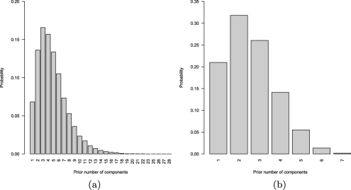
Figure 3: Prior number of clusters implied by our specification of $a$, $b$, $a_{1}$, $b_{1}$, $a_{2}$ and $b_{2}$. (a) $n=60$ (subject-level clustering), (b) $n=7$ (curve-level clustering).

To better understand the effect of our prior on $a$, $b$, $a_{1}$, $b_{1}$, $a_{2}$ and $b_{2}$, we show in Figure 3 the prior expected number of clusters implied by our choices. In particular, Figure 3(a) shows that, a priori, we expect between 1 and 8 clusters of subjects with high probability, with the most likely prior value being 3 clusters (note that this applies to both the mean-based and the distribution-based clustering methods). On the other hand, Figure 3(b) shows that, for a subject for which 7 cycles have been observed, we expect between 1 and 3 clusters with high probability. On the other hand, to assess the effect of the prior choices on the results, we conducted a small sensitivity analysis. In particular, the priors for $a$, $b$, $a_{1}$, $a_{2}$, $b_{1}$ and $b_{2}$ were replaced with exponential distributions with mean 2. The induced priors on the number of clusters have similar modes to our original specifications but have higher variability, placing substantially more mass on larger number of clusters. Although the posterior distribution for these parameters was somewhat affected, we did not see any substantial change in our posterior inferences on the clustering structure or the curve shapes (which are the main focus of our analysis). Similarly, we explored the effect of a $\mathsf{Beta}(1,1)$ prior on $\gamma$ and an $\mathsf{IGam}(2,0.1)$ prior on $\sigma^{2}$ without any significant change in the estimates of the hormonal profiles.

We start our analysis by comparing the clustering structure generated by the mean-based and distribution-based models considered in Section 4. For this purpose, we show in Figures 4 and 5 heatmaps of the average pairwise clustering probability matrix under these two models. Entry $(i,j)$ of the matrix contains the posterior probability that observations $i$ and $j$ are assigned to the same cluster. The black squares in the plots correspond to point estimates of the clustering structure obtained through the method described in Lau and Green (2007). In our case, the point estimate is obtained by minimizing a loss function that assigns equal weights to all pairwise misclassification errors. Therefore, the resulting plots provide information about the optimal clustering structure for the data as well as the uncertainty associated with it.

Figures 4 and 5 show that the structure of the clusters generated by both models are similar. For example, cluster 1 from mean-based clustering (counting from the bottom left corner of Figure 4) contains similar subjects as cluster 1 from distribution-based clustering (counting from the bottom left corner of Figure 5). The same is true for cluster 2 from both algorithms, and for cluster 5 from the mean-based clustering model and cluster 4 from the distribution-based model. There are also similarities in the structure of the outlier clusters (corresponding to the small clusters at the top and right of both heat maps). Both models assign subject 25 to a singleton cluster, while grouping subjects 21 and 53 into a pair, with subjects 40 and 51 in a separate pair. There are also some important differences between the two methods. Mean-based clustering groups subjects 36 and 43 together and assigns subject 3 to a different cluster (Figure 1 shows differences in the mean curve of subject 3), while distribution-based cluster groups subjects 3 and 43 together and assigns 36 to a different group. The behavior illustrates the robustness of distribution-based clustering, because except for a single outlier cycle for subject 43, the curves for this subject are much more similar to those of subject 3 than those of 36. Mean-based clustering also treats subjects 11 and 56 as singletons, while distribution-based clustering assigns them to the large cluster 4 (counting from the bottom left). Visually the raw profiles for subjects 11 and 56 are not very different from other profiles in cluster 4 [see panels (d), (e) and (f) of Figure 6], so this behavior seems reasonable.

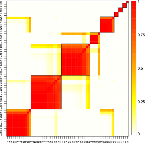
Figure 4: Average incidence matrix, illustrating probabilities of joint pairwise classification for the 60 women in the EPS under the mean-curve clustering procedure described in Section 4.1. White corresponds to zero probability, while red corresponds to 1. The squares correspond to a point estimate of the cluster structure in the data.

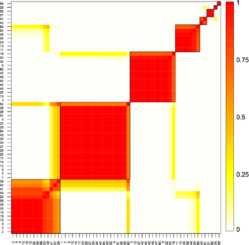
Figure 5: Average incidence matrix, illustrating probabilities of joint pairwise classification for the 60 women in the EPS under the distribution-based clustering procedure described in Section 4.2. White corresponds to zero probability, while red corresponds to 1. The squares correspond to a point estimate of the cluster structure in the data.

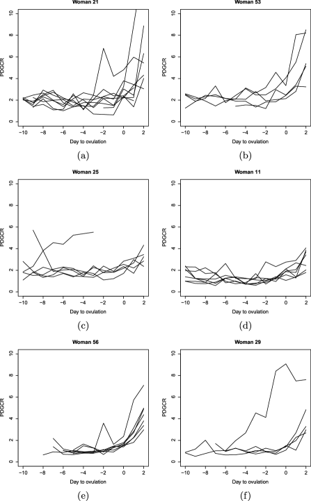
Figure 6: Raw data associated with the hormonal profiles for three outlier subjects in the Early Pregnancy Study.

Figure 7 shows reconstructed profiles under the distribution-based clustering model for some representative women in each of the main four groups. Most profiles are flat before ovulation, when hormone levels start to increase. Also, in most clusters the profiles tend to be relatively consistent for any single woman. However, we can see some outliers, typically corresponding to elevated post-ovulation levels and/or early increases in the hormone levels. Cluster 3 corresponds to women with very low hormonal levels, even after ovulation. This group has few outliers, and those present are characterized by a slightly larger increase in progesterone after ovulation, which is still under 1 µg$/$ml Cr. Group 2 shows much more diversity in the hormonal profiles, as well as a slightly higher baseline level in progesterone level and an earlier rise in progesterone than group 3. Group 1 tends to show few outliers, and otherwise differs from the previous ones in a higher baseline level and an early and very fast increase in progesterone. Finally, group 4 presents “normal” cycles with the highest baseline level of progesterone (1 µg$/$ml Cr) and the fastest increase in progesterone after ovulation, along with “abnormal” cycles with even higher baseline levels and very extreme levels of progesterone after ovulation (close to 5 µg$/$ml Cr).

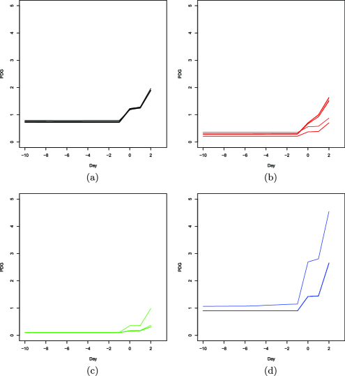
Figure 7: Reconstructed profiles for some representative subjects in the study. Panel (a) corresponds to patient 9 (who was chosen from cluster 1, counting from the bottom left), panel (b) to patient 36 (who was chosen from cluster 2), panel (c) to patient 45 (who was chosen from cluster 3), and panel (d) corresponds to patient 13 (who was chosen from cluster 4).

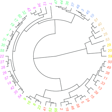
Figure 8: Dendogram for an alternative functional clustering algorithm that uses kernel smoothing to project all curves to a common set of grid knots and then applies complete-linkage hierarchical clustering and BIC to create a partition of the data.

For comparison we also applied a simple functional clustering approach based on kernel smoothing and hierarchical clustering. We first fitted a Gaussian kernel smoother [Li and Racine (2004), Racine and Li (2004)] to each of the curves, generated fitted values over a common grid (in this example we used 6 equally-spaced knots), then computed the average predicted values for each subject at each point of the grid, and finally applied complete-linkage hierarchical clustering (as implemented in the R package mclust), with the number of clusters selected using BIC. This approach identified 7 clusters; Figure 8 shows the associated dendogram, where colors are used to represent the clusters. Some of these clusters are similar to the ones identified by the mean-based clustering model. For example, the small cluster of 5 subjects (3, 10, 37, 45 and 48), corresponding to the fourth cluster from the bottom left in Figure 3, is perfectly identified by hierarchical clustering. Similarly, subjects 21, 25, 40, 51 and 53, which are all identified as outliers by the mean-based clustering model, are allocated to a single cluster by the hierarchical clustering approach. However, the majority of the clustering pattern generated by this method is quite different from the one obtained with mean-based or the distribution-based clustering. Furthermore, the number and structure of clusters depends heavily on the number and location of grid points used to interpolate the functions. For example, when the interpolation grid contains 5 knots we obtain 8 clusters, while 18 clusters are obtained when 11 knots are used for interpolation. Part of this difference could be due to the fact that, because most of the missing values tend to concentrate at the beginning of the cycle, many of the fitted functional values correspond to extrapolations rather than interpolations when a large number of knots are used.

We also note that posterior estimates of the precision parameters on the GDP suggest that a logarithmic rate of growth for the expected number of clusters might be reasonable for this data. For the mean-based clustering, the posterior mean for $a$ was $1.06$ and the 95% posterior symmetric credible interval was $(0.65,1.49)$, while the posterior mean for $b$ was $0.77$ with 95% credible interval $(0.17,1.72)$. For the distribution-based clustering, the corresponding estimates are $1.03$ $(0.62,1.56)$ and $0.72$ $(0.20,1.73)$ for $a_{1}$ and $b_{1}$, and $1.12$ $(0.71,1.43)$ and $0.27$ $(0.15,1.51)$ for $a_{2}$ and $b_{2}$.

Finally, we investigated the relationship between the clusters we identified using our distribution-based clustering algorithm and a series of covariates available for each subject, including age at the beginning of the study (Age), age of first menses (Age_Mense), average length of menses (Mense_Length), race (Race), body mass index (BMI), whether the subject had been taking contraceptives before the start of the study (EV_Pill) and whether the subject self reports as a consumer of marijuana during the period of the study (Marijuana_Use). To investigate this relationship, we used a classification tree, as implemented in the R package rpart. To simplify interpretation, we merged all the small outlier clusters into a single group (which we label cluster 5). The resulting classification tree (obtained using a Cp value of 0.03 for pruning) can be seen in Figure 9. Note that race and marijuana consumption do not appear to play any role in predicting the shape of the hormonal profiles. On the other hand, BMI, along with age, menses length and menses age, seems to have some predictive capability. For example, a BMI higher than 22 and an age of menses under 12 years old seem to predict progesterone profiles like the ones observed in cluster 3.

7 Discussion

We have presented two approaches to functional clustering in nested designs. These approaches look into different features of the nested samples and are therefore applicable in different circumstances. Our mean-based clustering approach is easier to interpret and provides an excellent alternative when within-subject samples are homogenous. However, when within-subject curves are heterogeneous, mean-based clustering can lead to biased results. Therefore, in studies such as the EPS, distribution-based models such as the one described here provide a viable alternative that acknowledges the heterogeneity in the function replicates from a subject.

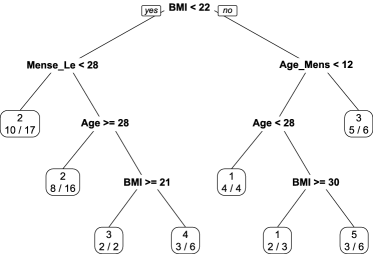
Figure 9: Classification tree explaining cluster membership on the basis of six covariates: age at the beginning of the study (Age), age of first menses (Age_Mense), average length of menses (Mense_Length), race (Race), body mass index (BMI), whether the subject had been taking contraceptives before the start of the study (EV_Pill) and whether the subject self reports as a consumer of marijuana during the period of the study (Marijuana_Use).

One interesting insight that can be gathered from the results of the EPS data is that, for small numbers of functional replicates per subject and rare outliers, the effect of the distribution-based clustering is to perform clustering based on the modal rather than the mean profile. That is, the distribution-based clustering model is able to automatically discount the abnormal curves, leading to more appropriate clustering patterns if the effect of outliers needs to be removed. Naturally, this perceived advantage of the distribution-based clustering method implicitly assumes that abnormal curves should be discounted. Although that assumption is justified in our application, users should be aware of it when applying our method to other data sets.

Appendix A Proof of Theorem 1

Let $\bolds{\theta}_{1}^{*},\bolds{\theta}_{2}^{*},\ldots$ be a sequence of independent and identically distributed samples from a random distribution $G$, which follows a $\mathsf{GDP}(a,b,G_{0})$ distribution. Also, let $W_{i}$ be 1 if $\bolds{\theta}^{*}_{i}$ is different from every $\bolds{\theta}_{1}^{*},\ldots,\bolds{\theta}^{*}_{i-1}$, and zero otherwise. Clearly, $Z_{n}=\sum_{i=1}^{n}W_{i}$ is the number of distinct values among the first $n$ samples form a $\mathsf{GDP}(a,b,G_{0})$. Hjort (2000) shows that

$$\mathsf{E}(W_{i}) = i\frac{\mathsf{E}\{u(1-u)^{i-1}\}}{1-\mathsf{E}\{(1-u)^{i}\}}$$

$$= i\frac{((\Gamma(a+b))/(\Gamma(a)\Gamma(b)))((\Gamma(a+1)\Gamma(b+i-1))/(\Gamma(a+b+i)))}{1-((\Gamma(a+b))/(\Gamma(a)\Gamma(b)))((\Gamma(a)\Gamma(b+i))(\Gamma(a+b+i)))}$$

$$= \frac{ia\Gamma(a+b)\Gamma(b+i-1)}{\Gamma(b)\Gamma(a+b+i)-\Gamma(a+b)\Gamma(b+i)},$$

which completes the proof.

Appendix B Truncations of generalized Dirichlet processes

Theorem 2

Assume that samples of $n$ observations have been collected for each of $J$ distributions and are contained in vector ${\mathbf{y}}=({\mathbf{y}}_{1}^{\prime},\ldots,{\mathbf{y}}_{J}^{\prime})$. Also, let

$$P^{\infty\infty}(\bolds{\theta}) = \int\!\!\int P(\bolds{\theta}|G_{j})P^{\infty}(dG_{j}|Q)P^{\infty}(dQ),$$

$$P^{LK}(\bolds{\theta}) = \int\!\!\int P(\bolds{\theta}|G_{j})P^{L}(dG_{j}|Q)P^{K}(dQ)$$

be, respectively, the prior distribution of the model parameters under the nested GDP model and its corresponding truncation after integrating out the random distributions, and $P^{\infty\infty}({\mathbf{y}})$ and $P^{LK}({\mathbf{y}})$ be the prior predictive distribution of the observations derived from these priors. Then

$$\int\bigl{|}P^{LK}({\mathbf{y}})-P^{\infty\infty}({\mathbf{y}})\bigr{|}\,d{\mathbf{y}}\leq\int\bigl{|}P^{LK}(\bolds{\theta})-P^{\infty\infty}(\bolds{\theta})\bigr{|}\leq\varepsilon^{LK}(\alpha,\beta),$$

where

$$\varepsilon^{LK}(\alpha,\beta) = \cases{\displaystyle 4\biggl{(}1-\biggl{[}1-\biggl{(}\frac{b_{1}}{a_{1}+b_{1}}\biggr{)}^{K-1}\biggr{]}^{J}\biggr{)},\hskip 25.0pt\mbox{if }L=\infty,K<\infty,\vspace*{8pt}\cr\displaystyle 4\biggl{(}1-\biggl{[}1-\biggl{(}\frac{b_{2}}{a_{2}+b_{2}}\biggr{)}^{L-1}\biggr{]}^{nJ}\biggr{)},\qquad\mbox{if }L<\infty,K=\infty,\vspace*{8pt}\cr\displaystyle 4\biggl{(}1-\biggl{[}1-\biggl{(}\frac{b_{1}}{a_{1}+b_{1}}\biggr{)}^{K-1}\biggr{]}^{J}\biggl{[}1-\biggl{(}\frac{b_{2}}{a_{2}+b_{2}}\biggr{)}^{L-1}\biggr{]}^{nJ}\biggr{)},\vspace*{5pt}\cr\hskip 170.0pt\mbox{if }L<\infty,K<\infty.}$$

The proof is a direct extension of results in Ishwaran and James (2001, 2002) and Rodríguez, Dunson and Gelfand (2008) and it is omitted for reasons of space. This result is particularly important since it justifies the use of computational algorithms based on finite mixtures and allows us to choose adequate truncation levels.

References

- Abraham et al. (2003) {barticle}[mr] \bauthor\bsnmAbraham, \bfnmC.\binitsC., \bauthor\bsnmCornillon, \bfnmP. A.\binitsP. A., \bauthor\bsnmMatzner-Løber, \bfnmE.\binitsE. and \bauthor\bsnmMolinari, \bfnmN.\binitsN. (\byear2003). \btitleUnsupervised curve clustering using B-splines. \bjournalScand. J. Stat. \bvolume30 \bpages581–595. \biddoi=10.1111/1467-9469.00350, issn=0303-6898, mr=2002229\bptokimsref\endbibitem
- Antoniak (1974) {barticle}[mr] \bauthor\bsnmAntoniak, \bfnmCharles E.\binitsC. E. (\byear1974). \btitleMixtures of Dirichlet processes with applications to Bayesian nonparametric problems. \bjournalAnn. Statist. \bvolume2 \bpages1152–1174. \bidissn=0090-5364, mr=0365969 \bptokimsref\endbibitem
- Bigelow and Dunson (2009) {barticle}[mr] \bauthor\bsnmBigelow, \bfnmJamie L.\binitsJ. L. and \bauthor\bsnmDunson, \bfnmDavid B.\binitsD. B. (\byear2009). \btitleBayesian semiparametric joint models for functional predictors. \bjournalJ. Amer. Statist. Assoc. \bvolume104 \bpages26–36. \biddoi=10.1198/jasa.2009.0001, issn=0162-1459, mr=2663031 \bptokimsref\endbibitem
- Booth, Casella and Hobert (2008) {barticle}[mr] \bauthor\bsnmBooth, \bfnmJames G.\binitsJ. G., \bauthor\bsnmCasella, \bfnmGeorge\binitsG. and \bauthor\bsnmHobert, \bfnmJames P.\binitsJ. P. (\byear2008). \btitleClustering using objective functions and stochastic search. \bjournalJ. R. Stat. Soc. Ser. B Stat. Methodol. \bvolume70 \bpages119–139. \biddoi=10.1111/j.1467-9868.2007.00629.x, issn=1369-7412, mr=2412634 \bptokimsref\endbibitem
- Brumback and Rice (1998) {barticle}[mr] \bauthor\bsnmBrumback, \bfnmBabette A.\binitsB. A. and \bauthor\bsnmRice, \bfnmJohn A.\binitsJ. A. (\byear1998). \btitleSmoothing spline models for the analysis of nested and crossed samples of curves. \bjournalJ. Amer. Statist. Assoc. \bvolume93 \bpages961–994. \biddoi=10.2307/2669837, issn=0162-1459, mr=1649194 \bptnotecheck related \bptokimsref\endbibitem
- Chiou and Li (2007) {barticle}[mr] \bauthor\bsnmChiou, \bfnmJeng-Min\binitsJ.-M. and \bauthor\bsnmLi, \bfnmPai-Ling\binitsP.-L. (\byear2007). \btitleFunctional clustering and identifying substructures of longitudinal data. \bjournalJ. R. Stat. Soc. Ser. B Stat. Methodol. \bvolume69 \bpages679–699. \biddoi=10.1111/j.1467-9868.2007.00605.x, issn=1369-7412, mr=2370075 \bptokimsref\endbibitem
- DiMatteo, Genovese and Kass (2001) {barticle}[mr] \bauthor\bsnmDiMatteo, \bfnmIlaria\binitsI., \bauthor\bsnmGenovese, \bfnmChristopher R.\binitsC. R. and \bauthor\bsnmKass, \bfnmRobert E.\binitsR. E. (\byear2001). \btitleBayesian curve-fitting with free-knot splines. \bjournalBiometrika \bvolume88 \bpages1055–1071. \biddoi=10.1093/biomet/88.4.1055, issn=0006-3444, mr=1872219 \bptokimsref\endbibitem
- Dunson (2009) {barticle}[mr] \bauthor\bsnmDunson, \bfnmDavid B.\binitsD. B. (\byear2009). \btitleNonparametric Bayes local partition models for random effects. \bjournalBiometrika \bvolume96 \bpages249–262. \biddoi=10.1093/biomet/asp021, issn=0006-3444, mr=2507141 \bptokimsref\endbibitem
- Dunson et al. (1999) {barticle}[pbm] \bauthor\bsnmDunson, \bfnmD. B.\binitsD. B., \bauthor\bsnmBaird, \bfnmD. D.\binitsD. D., \bauthor\bsnmWilcox, \bfnmA. J.\binitsA. J. and \bauthor\bsnmWeinberg, \bfnmC. R.\binitsC. R. (\byear1999). \btitleDay-specific probabilities of clinical pregnancy based on two studies with imperfect measures of ovulation. \bjournalHum. Reprod. \bvolume14 \bpages1835–1839. \bidissn=0268-1161, pmid=10402400 \bptokimsref\endbibitem
- Escobar and West (1995) {barticle}[mr] \bauthor\bsnmEscobar, \bfnmMichael D.\binitsM. D. and \bauthor\bsnmWest, \bfnmMike\binitsM. (\byear1995). \btitleBayesian density estimation and inference using mixtures. \bjournalJ. Amer. Statist. Assoc. \bvolume90 \bpages577–588. \bidissn=0162-1459, mr=1340510 \bptokimsref\endbibitem
- Ferguson (1973) {barticle}[mr] \bauthor\bsnmFerguson, \bfnmThomas S.\binitsT. S. (\byear1973). \btitleA Bayesian analysis of some nonparametric problems. \bjournalAnn. Statist. \bvolume1 \bpages209–230. \bidissn=0090-5364, mr=0350949 \bptokimsref\endbibitem
- Fraley and Raftery (2002) {barticle}[mr] \bauthor\bsnmFraley, \bfnmChris\binitsC. and \bauthor\bsnmRaftery, \bfnmAdrian E.\binitsA. E. (\byear2002). \btitleModel-based clustering, discriminant analysis, and density estimation. \bjournalJ. Amer. Statist. Assoc. \bvolume97 \bpages611–631. \biddoi=10.1198/016214502760047131, issn=0162-1459, mr=1951635 \bptokimsref\endbibitem
- García-Escudero and Gordaliza (2005) {barticle}[mr] \bauthor\bsnmGarcía-Escudero, \bfnmLuis Angel\binitsL. A. and \bauthor\bsnmGordaliza, \bfnmAlfonso\binitsA. (\byear2005). \btitleA proposal for robust curve clustering. \bjournalJ. Classification \bvolume22 \bpages185–201. \biddoi=10.1007/s00357-005-0013-8, issn=0176-4268, mr=2231171 \bptokimsref\endbibitem
- Gelman and Rubin (1992) {barticle}[auto:STB—2014/06/18—12:29:53] \bauthor\bsnmGelman, \bfnmA.\binitsA. and \bauthor\bsnmRubin, \bfnmD.\binitsD. (\byear1992). \btitleInferences from iterative simulation using multiple sequences. \bjournalStatist. Sci. \bvolume7 \bpages457–472. \bptokimsref\endbibitem
- Heard, Holmes and Stephens (2006) {barticle}[mr] \bauthor\bsnmHeard, \bfnmNicholas A.\binitsN. A., \bauthor\bsnmHolmes, \bfnmChristopher C.\binitsC. C. and \bauthor\bsnmStephens, \bfnmDavid A.\binitsD. A. (\byear2006). \btitleA quantitative study of gene regulation involved in the immune response of anopheline mosquitoes: An application of Bayesian hierarchical clustering of curves. \bjournalJ. Amer. Statist. Assoc. \bvolume101 \bpages18–29. \biddoi=10.1198/016214505000000187, issn=0162-1459, mr=2252430 \bptokimsref\endbibitem
- Hjort (2000) {bmisc}[auto:STB—2014/06/18—12:29:53] \bauthor\bsnmHjort, \bfnmN.\binitsN. (\byear2000). \bhowpublishedBayesian analysis for a generalized Dirichlet process prior. Technical report, Univ. Oslo. \bptokimsref\endbibitem
- Ishwaran and James (2001) {barticle}[mr] \bauthor\bsnmIshwaran, \bfnmHemant\binitsH. and \bauthor\bsnmJames, \bfnmLancelot F.\binitsL. F. (\byear2001). \btitleGibbs sampling methods for stick-breaking priors. \bjournalJ. Amer. Statist. Assoc. \bvolume96 \bpages161–173. \biddoi=10.1198/016214501750332758, issn=0162-1459, mr=1952729 \bptokimsref\endbibitem
- Ishwaran and James (2002) {barticle}[mr] \bauthor\bsnmIshwaran, \bfnmHemant\binitsH. and \bauthor\bsnmJames, \bfnmLancelot F.\binitsL. F. (\byear2002). \btitleApproximate Dirichlet process computing in finite normal mixtures: Smoothing and prior information. \bjournalJ. Comput. Graph. Statist. \bvolume11 \bpages508–532. \biddoi=10.1198/106186002411, issn=1061-8600, mr=1938445 \bptokimsref\endbibitem
- James and Sugar (2003) {barticle}[mr] \bauthor\bsnmJames, \bfnmGareth M.\binitsG. M. and \bauthor\bsnmSugar, \bfnmCatherine A.\binitsC. A. (\byear2003). \btitleClustering for sparsely sampled functional data. \bjournalJ. Amer. Statist. Assoc. \bvolume98 \bpages397–408. \biddoi=10.1198/016214503000189, issn=0162-1459, mr=1995716 \bptokimsref\endbibitem
- Lau and Green (2007) {barticle}[mr] \bauthor\bsnmLau, \bfnmJohn W.\binitsJ. W. and \bauthor\bsnmGreen, \bfnmPeter J.\binitsP. J. (\byear2007). \btitleBayesian model-based clustering procedures. \bjournalJ. Comput. Graph. Statist. \bvolume16 \bpages526–558. \biddoi=10.1198/106186007X238855, issn=1061-8600, mr=2351079 \bptokimsref\endbibitem
- Li (2005) {barticle}[mr] \bauthor\bsnmLi, \bfnmJia\binitsJ. (\byear2005). \btitleClustering based on a multilayer mixture model. \bjournalJ. Comput. Graph. Statist. \bvolume14 \bpages547–568. \biddoi=10.1198/106186005X59586, issn=1061-8600, mr=2170201 \bptokimsref\endbibitem
- Li and Racine (2004) {barticle}[mr] \bauthor\bsnmLi, \bfnmQi\binitsQ. and \bauthor\bsnmRacine, \bfnmJeff\binitsJ. (\byear2004). \btitleCross-validated local linear nonparametric regression. \bjournalStatist. Sinica \bvolume14 \bpages485–512. \bidissn=1017-0405, mr=2059293 \bptokimsref\endbibitem
- Liang et al. (2008) {barticle}[mr] \bauthor\bsnmLiang, \bfnmFeng\binitsF., \bauthor\bsnmPaulo, \bfnmRui\binitsR., \bauthor\bsnmMolina, \bfnmGerman\binitsG., \bauthor\bsnmClyde, \bfnmMerlise A.\binitsM. A. and \bauthor\bsnmBerger, \bfnmJim O.\binitsJ. O. (\byear2008). \btitleMixtures of priors for Bayesian variable selection. \bjournalJ. Amer. Statist. Assoc. \bvolume103 \bpages410–423. \biddoi=10.1198/016214507000001337, issn=0162-1459, mr=2420243 \bptokimsref\endbibitem
- Luan and Li (2003) {barticle}[auto:STB—2014/06/18—12:29:53] \bauthor\bsnmLuan, \bfnmY.\binitsY. and \bauthor\bsnmLi, \bfnmH.\binitsH. (\byear2003). \btitleClustering of time-course gene expression data using a mixed effects model with b-splines. \bjournalBioinformatics \bvolume19 \bpages474–482. \bptokimsref\endbibitem
- McCloskey (1965) {bmisc}[mr] \bauthor\bsnmMcCloskey, \bfnmJohn William Thomas\binitsJ. W. T. (\byear1965). \bhowpublishedA model for the distribution of individuals by species in an environment. Ph.D. thesis, Michigan State Univ. \bidmr=2615013 \bptokimsref\endbibitem
- Medvedovic and Sivaganesan (2002) {barticle}[pbm] \bauthor\bsnmMedvedovic, \bfnmMario\binitsM. and \bauthor\bsnmSivaganesan, \bfnmSiva\binitsS. (\byear2002). \btitleBayesian infinite mixture model based clustering of gene expression profiles. \bjournalBioinformatics \bvolume18 \bpages1194–1206. \bidissn=1367-4803, pmid=12217911 \bptokimsref\endbibitem
- Ongaro and Cattaneo (2004) {barticle}[mr] \bauthor\bsnmOngaro, \bfnmAndrea\binitsA. and \bauthor\bsnmCattaneo, \bfnmCarla\binitsC. (\byear2004). \btitleDiscrete random probability measures: A general framework for nonparametric Bayesian inference. \bjournalStatist. Probab. Lett. \bvolume67 \bpages33–45. \biddoi=10.1016/j.spl.2003.11.014, issn=0167-7152, mr=2039931 \bptokimsref\endbibitem
- Paciorek (2006) {barticle}[mr] \bauthor\bsnmPaciorek, \bfnmChristopher J.\binitsC. J. (\byear2006). \btitleMisinformation in the conjugate prior for the linear model with implications for free-knot spline modelling. \bjournalBayesian Anal. \bvolume1 \bpages375–383 (electronic). \biddoi=10.1214/06-BA114, mr=2221270 \bptokimsref\endbibitem
- Pitman (1995) {barticle}[mr] \bauthor\bsnmPitman, \bfnmJim\binitsJ. (\byear1995). \btitleExchangeable and partially exchangeable random partitions. \bjournalProbab. Theory Related Fields \bvolume102 \bpages145–158. \biddoi=10.1007/BF01213386, issn=0178-8051, mr=1337249 \bptokimsref\endbibitem
- Pitman (1996) {bincollection}[mr] \bauthor\bsnmPitman, \bfnmJim\binitsJ. (\byear1996). \btitleSome developments of the Blackwell–MacQueen urn scheme. In \bbooktitleStatistics, Probability and Game Theory. Papers in Honor of David Blackwell (\beditor\bfnmT. S.\binitsT. S. \bsnmFerguson, \beditor\bfnmL. S.\binitsL. S. \bsnmShapeley and \beditor\bfnmJ. B.\binitsJ. B. \bsnmMacQueen, eds.) \bpages245–267. \bpublisherIMS, \blocationHayward, CA. \biddoi=10.1214/lnms/1215453576, mr=1481784 \bptokimsref\endbibitem
- Quintana and Iglesias (2003) {barticle}[mr] \bauthor\bsnmQuintana, \bfnmFernando A.\binitsF. A. and \bauthor\bsnmIglesias, \bfnmPilar L.\binitsP. L. (\byear2003). \btitleBayesian clustering and product partition models. \bjournalJ. R. Stat. Soc. Ser. B Stat. Methodol. \bvolume65 \bpages557–574. \biddoi=10.1111/1467-9868.00402, issn=1369-7412, mr=1983764 \bptokimsref\endbibitem
- Racine and Li (2004) {barticle}[mr] \bauthor\bsnmRacine, \bfnmJeff\binitsJ. and \bauthor\bsnmLi, \bfnmQi\binitsQ. (\byear2004). \btitleNonparametric estimation of regression functions with both categorical and continuous data. \bjournalJ. Econometrics \bvolume119 \bpages99–130. \biddoi=10.1016/S0304-4076(03)00157-X, issn=0304-4076, mr=2041894 \bptokimsref\endbibitem
- Ramoni, Sebastiani and Kohane (2002) {barticle}[mr] \bauthor\bsnmRamoni, \bfnmMarco F.\binitsM. F., \bauthor\bsnmSebastiani, \bfnmPaola\binitsP. and \bauthor\bsnmKohane, \bfnmIsaac S.\binitsI. S. (\byear2002). \btitleCluster analysis of gene expression dynamics. \bjournalProc. Natl. Acad. Sci. USA \bvolume99 \bpages9121–9126 (electronic). \biddoi=10.1073/pnas.132656399, issn=1091-6490, mr=1909705 \bptokimsref\endbibitem
- Ramsay and Silverman (2005) {bbook}[mr] \bauthor\bsnmRamsay, \bfnmJ. O.\binitsJ. O. and \bauthor\bsnmSilverman, \bfnmB. W.\binitsB. W. (\byear2005). \btitleFunctional Data Analysis, \bedition2nd ed. \bpublisherSpringer, \blocationNew York. \bidmr=2168993 \bptokimsref\endbibitem
- Ray and Mallick (2006) {barticle}[mr] \bauthor\bsnmRay, \bfnmShubhankar\binitsS. and \bauthor\bsnmMallick, \bfnmBani\binitsB. (\byear2006). \btitleFunctional clustering by Bayesian wavelet methods. \bjournalJ. R. Stat. Soc. Ser. B Stat. Methodol. \bvolume68 \bpages305–332. \biddoi=10.1111/j.1467-9868.2006.00545.x, issn=1369-7412, mr=2188987 \bptokimsref\endbibitem
- Robert and Casella (1999) {bbook}[mr] \bauthor\bsnmRobert, \bfnmChristian P.\binitsC. P. and \bauthor\bsnmCasella, \bfnmGeorge\binitsG. (\byear1999). \btitleMonte Carlo Statistical Methods. \bpublisherSpringer, \blocationNew York. \biddoi=10.1007/978-1-4757-3071-5, mr=1707311 \bptokimsref\endbibitem
- Rodriguez and Dunson (2014) {bmisc}[author] \bauthor\bsnmRodriguez, \binitsA. and \bauthor\bsnmDunson, \binitsD. B. (\byear2014). \bhowpublishedSupplement to “Functional clustering in nested designs: Modeling variability in reproductive epidemiology studies.” DOI:\doiurl10.1214/14-AOAS751SUPP. \bptokimsref \endbibitem
- Rodríguez, Dunson and Gelfand (2008) {barticle}[mr] \bauthor\bsnmRodríguez, \bfnmAbel\binitsA., \bauthor\bsnmDunson, \bfnmDavid B.\binitsD. B. and \bauthor\bsnmGelfand, \bfnmAlan E.\binitsA. E. (\byear2008). \btitleThe nested Dirichlet process. \bjournalJ. Amer. Statist. Assoc. \bvolume103 \bpages1131–1144. \biddoi=10.1198/016214508000000553, issn=0162-1459, mr=2528831 \bptnotecheck related \bptokimsref\endbibitem
- Rodríguez, Dunson and Gelfand (2009) {barticle}[mr] \bauthor\bsnmRodríguez, \bfnmAbel\binitsA., \bauthor\bsnmDunson, \bfnmDavid B.\binitsD. B. and \bauthor\bsnmGelfand, \bfnmAlan E.\binitsA. E. (\byear2009). \btitleBayesian nonparametric functional data analysis through density estimation. \bjournalBiometrika \bvolume96 \bpages149–162. \biddoi=10.1093/biomet/asn054, issn=0006-3444, mr=2482141 \bptokimsref\endbibitem
- Serban and Wasserman (2005) {barticle}[mr] \bauthor\bsnmSerban, \bfnmNicoleta\binitsN. and \bauthor\bsnmWasserman, \bfnmLarry\binitsL. (\byear2005). \btitleCATS: Clustering after transformation and smoothing. \bjournalJ. Amer. Statist. Assoc. \bvolume100 \bpages990–999. \biddoi=10.1198/016214504000001574, issn=0162-1459, mr=2201025 \bptokimsref\endbibitem
- Sethuraman (1994) {barticle}[mr] \bauthor\bsnmSethuraman, \bfnmJayaram\binitsJ. (\byear1994). \btitleA constructive definition of Dirichlet priors. \bjournalStatist. Sinica \bvolume4 \bpages639–650. \bidissn=1017-0405, mr=1309433 \bptokimsref\endbibitem
- Smith and Kohn (1996) {barticle}[auto:STB—2014/06/18—12:29:53] \bauthor\bsnmSmith, \bfnmM.\binitsM. and \bauthor\bsnmKohn, \bfnmR.\binitsR. (\byear1996). \btitleNonparametric regression using Bayesian variable selection. \bjournalJ. Econometrics \bvolume75 \bpages317–343. \bptokimsref\endbibitem
- Sudderth and Jordan (2009) {bincollection}[auto:STB—2014/06/18—12:29:53] \bauthor\bsnmSudderth, \bfnmE. B.\binitsE. B. and \bauthor\bsnmJordan, \bfnmM. I.\binitsM. I. (\byear2009). \btitleShared segmentation of natural scenes using dependent Pitman–Yor processes. In \bbooktitleAdvances in Neural Information Processing Systems 21 (\beditor\bfnmD.\binitsD. \bsnmKoller, \beditor\bfnmD.\binitsD. \bsnmSchuurmans, \beditor\bfnmY.\binitsY. \bsnmBengio and \beditor\bfnmL.\binitsL. \bsnmBottou, eds.). \bptokimsref\endbibitem
- Tarpey and Kinateder (2003) {barticle}[mr] \bauthor\bsnmTarpey, \bfnmThaddeus\binitsT. and \bauthor\bsnmKinateder, \bfnmKimberly K. J.\binitsK. K. J. (\byear2003). \btitleClustering functional data. \bjournalJ. Classification \bvolume20 \bpages93–114. \biddoi=10.1007/s00357-003-0007-3, issn=0176-4268, mr=1983123 \bptokimsref\endbibitem
- Wakefield, Zhou and Self (2003) {bincollection}[mr] \bauthor\bsnmWakefield, \bfnmJon C.\binitsJ. C., \bauthor\bsnmZhou, \bfnmChuan\binitsC. and \bauthor\bsnmSelf, \bfnmSteve G.\binitsS. G. (\byear2003). \btitleModelling gene expression data over time: Curve clustering with informative prior distributions. In \bbooktitleBayesian Statistics, 7 (Tenerife, 2002) (\beditor\bfnmJ.\binitsJ. \bsnmBernardo, \beditor\bfnmM.\binitsM. \bsnmBayarri, \beditor\bfnmJ.\binitsJ. \bsnmBerger, \beditor\bfnmA.\binitsA. \bsnmDawid, \beditor\bfnmD.\binitsD. \bsnmHeckerman, \beditor\bfnmA.\binitsA. \bsnmSmith and \beditor\bfnmM.\binitsM. \bsnmWest, eds.) \bpages721–732. \bpublisherOxford Univ. Press, \blocationNew York. \bidmr=2003536 \bptokimsref\endbibitem
- Wilcox et al. (1998) {barticle}[auto:STB—2014/06/18—12:29:53] \bauthor\bsnmWilcox, \bfnmA. J.\binitsA. J., \bauthor\bsnmWeinberg, \bfnmC. R.\binitsC. R., \bauthor\bsnmO’Connor, \bfnmJ. F.\binitsJ. F., \bauthor\bsnmBaid, \bfnmD. D.\binitsD. D., \bauthor\bsnmSchlatterer, \bfnmJ. P.\binitsJ. P., \bauthor\bsnmCanfield, \bfnmR. E.\binitsR. E., \bauthor\bsnmArmstrong, \bfnmE. G.\binitsE. G. and \bauthor\bsnmNisula, \bfnmB. C.\binitsB. C. (\byear1998). \btitleIncidence of early loss of pregnancy. \bjournalN. Engl. J. Med. \bvolume319 \bpages189–194. \bptokimsref\endbibitem
- Yeung and Ruzzo (2001) {barticle}[pbm] \bauthor\bsnmYeung, \bfnmK. Y.\binitsK. Y. and \bauthor\bsnmRuzzo, \bfnmW. L.\binitsW. L. (\byear2001). \btitlePrincipal component analysis for clustering gene expression data. \bjournalBioinformatics \bvolume17 \bpages763–774. \bidissn=1367-4803, pmid=11590094 \bptokimsref\endbibitem
- Yeung et al. (2001) {barticle}[auto:STB—2014/06/18—12:29:53] \bauthor\bsnmYeung, \bfnmK. Y.\binitsK. Y., \bauthor\bsnmFraley, \bfnmC.\binitsC., \bauthor\bsnmMuruan, \bfnmA.\binitsA., \bauthor\bsnmRaftery, \bfnmA. E.\binitsA. E. and \bauthor\bsnmRuzzo, \bfnmW. L.\binitsW. L. (\byear2001). \btitleModel-based clustering and data transformation for gene expression data. \bjournalBioinformatics \bvolume17 \bpages977–987. \bptokimsref\endbibitem