The Laplacian polynomial of graphs derived from regular graphs and applications

Abstract

Let $R(G)$ be the graph obtained from $G$ by adding a new vertex corresponding to each edge of $G$ and by joining each new vertex to the end vertices of the corresponding edge. Let $RT(G)$ be the graph obtained from $R(G)$ by adding a new edge corresponding to every vertex of $G$, and by joining each new edge to every vertex of $G$. In this paper, we determine the Laplacian polynomials of $RT(G)$ of a regular graph $G$. Moreover, we derive formulae and lower bounds of Kirchhoff index of the graphs. Finally we also present the formulae for calculating the Kirchhoff index of some special graphs as applications, which show the correction and efficiency of the proposed results.

1 Introduction

All graphs considered in this paper are simple and undirected. Let $G=(V(G),E(G))$ be a graph with vertex set $V(E)=\{v_{1},v_{2},\dots,v_{n}\}$ and edge set $E(G)=\{e_{1},e_{2},\dots,e_{m}\}$. The adjacency matrix of $G$, denoted by $A(G)$, is the $n\times n$ matrix whose $(i,j)$-entry is $1$ if $v_{i}$ and $v_{j}$ are adjacent in $G$ and $0$ otherwise. Let $B(G)$ denote the adjacency matrix and vertex-edge incidence matrix of $G$, which is the $n\times m$ matrix whose $(i,j)$-entry is $1$ if $v_{i}$ is incident to $e_{j}$ and $0$ otherwise. Denote $D(G)$ to be the diagonal matrix with diagonal entries $d_{G}(v_{1}),d_{G}(v_{2}),\dots,d_{G}(v_{n}).$ The Laplacian matrix of $G$ defined as $L(G)=D(G)-A(G)$. The Laplacian characteristic polynomial of $L(G)$, is defined as

$$\phi(L(G);x)=det(xI_{n}-L(G)),$$

or simply $\phi(L)$, where $I_{n}$ is the identity matrix of size $n$, and its roots, denoted by $0=\mu_{1}(G)\leq\mu_{2}(G)\leq\dots\leq\mu_{n}(G),$ are called the Laplacian eigenvalues of $G$. The collection of eigenvalues of $L(G)$ together with their multiplicities are called the $L$-spectrum of $G$. Similar terminology will be used for $A(G).$ The adjacency characteristic polynomial of $G$, denoted by $\varphi(A(G);x)$, is defined as

$$\varphi(A(G);x)=det(xI_{n}-A(G)),$$

the eigenvalues of $A(G)$ are $\lambda_{1}(G)\geq\lambda_{2}(G)\geq\dots\geq\lambda_{n}(G)$. The collection of eigenvalues of $A(G)$ together with their multiplicities are called the $A$-spectrum of $G$. For other undefined notations and terminology from graph theory, the readers may refer to [1] and the references therein.

Klein and Randić [2] introduced a new distance function named resistance distance based on electrical network theory. The resistance distance between vertices $i$ and $j$, denoted by $r_{ij}$, is defined to be the effective electrical resistance between them if each edge of $G$ is replaced by a unit resistor [2]. The resistance distances attracted extensive attention due to its wide applications in physics, chemistry, etc. [3, 4, 5, 6, 24]. For more information on resistance distances of graphs, the readers are referred to the recent papers  [7, 8, 25].

Until now, a large amount of graph operations such as the Cartesian product, the Kronecker product, the corona and neighborhood corona graphs have been introduced in [16, 17, 18, 19, 20]. The following definition comes from [1] (see the definition in p. 63 in [1]).

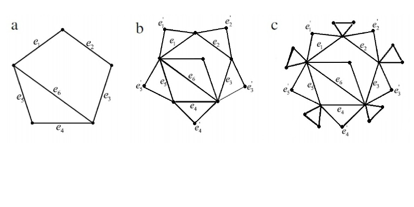
Figure 1: (a) The graph $G$.   (b) The graph $R(G)$.   (c) The graph $RT(G)$.

Definition 1.1

(see [1]) Let $R(G)=(V(R(G)),E(R(G)))$ be the graph obtained from $G$ by adding a new vertex $e^{\prime}$ corresponding to each edge $e=(a,b)$ of $G$ and by joining each new vertex $e^{\prime}$ to the end vertices $a$ and $b$ of the corresponding edge $e=(a,b).$ (see Fig. 1(a) and (b) for example).

From the above definition, it is obvious that $R(G)$ is obtained from $G$ by “changing each edge $e=(a,b)$ of $G$ into a triangle $ae^{\prime}b$”. Thus, $V(R(G))=V(G)\cup\{e^{\prime}\mid e\in E(G)\}$ and $E(R(G))=E(G)\cup\{(v_{i},e^{\prime}),(v_{j},e^{\prime})\mid e=(v_{i},v_{j})\in E(G)\}$. A very elementary and natural question is what it would be like if we change each edge and each vertex of $G$ into a triangle, which is stated as the following definiton.

Definition 1.2

Let $RT(G)=(V(RT(G)),E(RT(G)))$ be the graph obtained from $RG$ by adding a new edge $e^{\prime\prime}_{i}=(w^{i}_{1},w^{i}_{2})$ corresponding to each vertex $v_{i}$ of $G$ and by joining the two vertices of each new edge to each vertex $v_{i}$ of $G$, $RT(G)$ is obtained from $G$ by “changing each edge and each vertex of $G$ into a triangle”. Thus, $V(RT(G))=\{e^{\prime}\mid e\in E(G)\}\cup V(G)\cup\{w_{1}^{i}\mid i=1,2,\dots,n\}\cup\{w_{2}^{i}\mid i=1,2,\dots,n\}$ and $E(RT(G))=\{(v_{i},e^{\prime}),(v_{j},e^{\prime})\mid e=(v_{i},v_{j})\in E(G)\}\cup E(G)\cup\{(v_{i},w_{1}^{i}),(v_{i},w_{2}^{i})\mid v_{i}\in V(G),e^{\prime\prime}_{i}=(w^{i}_{1},w^{i}_{2})\in E(RT(G)),i=1,2,\dots,n\}$.(see Fig. 1(a), (b) and (c) for example).

As the authors of [10] pointed out, it is an interesting problem to study the Kirchhoff index of graphs derived from a single graph. In [11], the authors obtained formulae and lower bounds of the Kirchhoff index of the line graph, subdivision graph, total graph of a connected regular graph, respectively. In [12], Wang et al. determined the Laplacian polynomials of $R(G)$ and $Q(G)$ of a regular graph $G$, they also derived formulae and lower bounds of the Kirchhoff index of those graphs. Motivated by the results, in this paper we further explore the Laplacian polynomials of $RT(G)$ of a regular graph $G$. Moreover, we derive the formulae and lower bounds of Kirchhoff index of the graphs. In particular, special formulae are proposed for the Kirchhoff index of $RT(G)$, where $G$ is a complete graph $K_{n}$, a cycle $C_{n}$ and a regular complete bipartite graph $K_{n,n}$.

2 Preliminaries

At the beginning of this section, we review some concepts in matrix theory. The Kronecker product $A\bigotimes B$ of two matrices $A=(a_{ij})_{m\times n}$ and $B=(b_{ij})_{p\times q}$ is the $mp\times nq$ matrix obtained from $A$ by replacing each element $a_{ij}$ by $a_{ij}B$. If $A,B,C$ and $D$ are matrices of such size that one can form the matrix products $AC$ and $BD$, then $(A\bigotimes B)(C\bigotimes D)=AC\bigotimes BD.$ It follows that $A\bigotimes B$ is invertible if and only if $A$ and $B$ are invertible, in which case the inverse is given by $(A\bigotimes B)^{-1}=A^{-1}\bigotimes B^{-1}.$ Note also that $(A\bigotimes B)^{T}=A^{T}\bigotimes B^{T}$. Moreover, if the matrices $A$ and $B$ are of order $n\times n$ and $p\times p$, respectively, then $det(A\bigotimes B)=(det~{}A)^{p}(det~{}B)^{n}.$ The readers are referred to [21] for other properties of the Kronecker product not mentioned here.

The symbols $\mathbf{0}_{n}$ and $\mathbf{1}_{n}$ (resp., $\mathbf{0}_{mn}$ and $\mathbf{1}_{mn}$) will stand for the length-n column vectors (resp. $m\times n$ matrices) consisting entirely of 0’s and 1’s.

Lemma 2.1

(see [9]) Let $M_{1},M_{2},M_{3}$ and $M_{4}$ be respectively $p\times p$, $p\times q$, $q\times p$ and $q\times q$ matrices with $M_{1}$ and $M_{4}$ invertible, then

$$det\left[\begin{array}[]{cc}M_{1}&M_{2}\\ M_{3}&M_{4}\\ \end{array}\right] =det(M_{4})\cdot det(M_{1}-M_{2}M_{4}^{-1}M_{3})$$ (4)

$$=det(M_{1})\cdot det(M_{4}-M_{3}M_{1}^{-1}M_{2}),$$

where $M_{1}-M_{2}M_{4}^{-1}M_{3}$ and $M_{4}-M_{3}M_{1}^{-1}M_{2}$ are called the Schur complements of $M_{4}$ and $M_{1}$, respectively.

3 The Laplacian polynomials of RT(G)

For a regular graph $G$, the following theorem gives the representation of the Laplacian polynomial of $RT(G)$ by means of the characteristic polynomial and the Laplacian polynomial of $G$, respectively.

Theorem 3.1

Let $G$ be an $r$-regular graph with $n$ vertices and $m$ edges, then $(i)~{}\phi\Big{(}RT(G);\mu\Big{)}\\ =(\mu-1)^{n}(\mu-2)^{m-n}(\mu-3)^{n}(3-\mu)^{n}\varphi\Big{(}G;\frac{(\mu-2)^{2}}{3-\mu}+\frac{r(2\mu-3)}{\mu-3}+\frac{2(\mu-2)}{(\mu-1)(\mu-3)}\Big{)}.$ $(ii)~{}\phi\Big{(}RT(G);\mu\Big{)}=(\mu-1)^{n}(\mu-2)^{m-n}(\mu-3)^{2n}\phi\Big{(}G;\frac{(\mu-2)^{2}}{\mu-3}-\frac{r\mu}{\mu-3}-\frac{2(\mu-2)}{(\mu-1)(\mu-3)}\Big{)}.$

Proof. (i) Let $G$ be an arbitrary $r$-regular graph with $n$ vertices and $m$ edges. Label the vertices of $RT(G)$ as follows. Let $I(G)=\{e_{1},e_{2},\dots,e_{m}\}$, $V(G)=\{v_{1},v_{2},\dots,v_{n}\}$ and $V(e^{\prime\prime})=\{w_{1},w_{2}\}$, and let $w^{i}_{1},w^{i}_{2}$ denote the vertices of the $i$-th copy of $e^{\prime\prime}$ for $i=1,2,\dots,n$, with the understanding that $w^{i}_{j}$ is the copy of $w_{j}$ for each $j$. Denote $W_{j}=\{w^{1}_{j},w^{2}_{j},\dots,w^{n}_{j}\}$, for $j=1,2$, then

$$I(G)\bigcup V(G)\bigcup\big{[}W_{1}\bigcup W_{2}\big{]}$$ (5)

is a partition of $V(RT(G))$. Obviously, the degrees of the vertices of $RT(G)$ are: $d_{RT(G)}(e_{i})=2$, for $i=1,2,\dots,m$,
$~{}~{}~{}~{}~{}~{}~{}d_{RT(G)}(v_{i})=2d_{G}(v_{i})+2$, for $i=1,2,\dots,n$,
and $d_{RT(G)}(w_{j}^{i})=2$, for $i=1,2,\dots,n,j=1,2$.

Let $B$ denotes vertex-edge incidence matrix of $G$. Since $G$ is an $r$-regular graph, we have $D(G)=rI_{n}$. With respect to the partition (3), then the Laplacian matrix of $RT(G)$ can be written as

$$L(RT(G))=\left[\begin{array}[]{cc|lr}2I_{m}&-B^{T}&~{}~{}~{}~{}~{}~{}~{}~{}0_{m\times 2n}\\ -B&L(G)+(r+2)I_{n}&~{}~{}~{}~{}~{}-I_{n}\otimes\mathbf{1}^{T}_{2}\\ \hline\cr~{}~{}0_{2n\times m}&-I_{n}\otimes\mathbf{1}_{2}&~{}I_{n_{1}}\otimes\left[\begin{array}[]{cc}2&-1\\ -1&2\\ \end{array}\right]\\ \end{array}\right],$$

where $\mathbf{1}_{n}$ denotes the all-one column vector with size $n$.

By Lemma 2.1, we have

$$\phi\Big{(}RT(G);\mu\Big{)}$$

$$=det\left[\begin{array}[]{cc|lr}(\mu-2)I_{m}&B^{T}&~{}~{}~{}~{}~{}~{}~{}~{}0_{m\times 2n}\\ B&(\mu-r-2)I_{n}-L(G)&~{}~{}~{}~{}~{}I_{n}\otimes\mathbf{1}^{T}_{2}\\ \hline\cr~{}~{}0_{2n\times m}&I_{n}\otimes\mathbf{1}_{2}&~{}I_{n}\otimes\left[\begin{array}[]{cc}\mu-2&1\\ 1&\mu-2\\ \end{array}\right]\\ \end{array}\right]$$ (10)

$$=det\Bigg{[}I_{n_{1}}\otimes\left[\begin{array}[]{cc}\mu-2&1\\ 1&\mu-2\\ \end{array}\right]\Bigg{]}\cdot det~{}S$$ (13)

$$=(\mu-1)^{n}(\mu-3)^{n}\cdot det~{}S,$$ (14)

where

$$S$$

$$=\left[\begin{array}[]{cc}(\mu-2)I_{m}&B^{T}\\ B&(\mu-r-2)I_{n}-L(G)\\ \end{array}\right]-\left[\begin{array}[]{c}\mathbf{0}_{0\times 2n}\\ I_{n}\otimes\mathbf{1}_{2}^{T}\\ \end{array}\right]$$

$$~{}~{}~{}\cdot\left[\begin{array}[]{c}I_{n_{1}}\otimes\left[\begin{array}[]{cc}\mu-2&1\\ 1&\mu-2\\ \end{array}\right]\\ \end{array}\right]^{-1}\left[\begin{array}[]{cc}\mathbf{0}_{2n\times m}&I_{n}\otimes\mathbf{1}_{2}\\ \end{array}\right]$$

$$=\left[\begin{array}[]{cc}(\mu-2)I_{m}&B^{T}\\ B&(\mu-r-2)I_{n}-L(G)\\ \end{array}\right]-\left[\begin{array}[]{c}\mathbf{0}_{0\times 2n}\\ I_{n}\otimes\mathbf{1}_{2}^{T}\\ \end{array}\right]$$

$$~{}~{}~{}\cdot\left[\begin{array}[]{c}I_{n}\otimes\left[\begin{array}[]{cc}\mu-2&1\\ 1&\mu-2\\ \end{array}\right]\\ \end{array}^{-1}\right]\left[\begin{array}[]{cc}\mathbf{0}_{2n\times m}&I_{n}\otimes\mathbf{1}_{2}\\ \end{array}\right]$$

$$=\left[\begin{array}[]{cc}(\mu-2)I_{m}&B^{T}\\ B&(\mu-r-2)I_{n}-L(G)\\ \end{array}\right]$$

$$~{}~{}-\left[\begin{array}[]{cc}\mathbf{0}_{m\times m}&\mathbf{0}_{m\times n}\\ \mathbf{0}_{n\times m}&I_{n}\otimes\mathbf{1}_{2}^{T}\left[\begin{array}[]{cc}\mu-2&1\\ 1&\mu-2\\ \end{array}\right]^{-1}\mathbf{1}_{2}\\ \end{array}\right]$$

$$=\left[\begin{array}[]{cc}(\mu-2)I_{m}&B^{T}\\ B&(\mu-r-2)I_{n}-L(G)\\ \end{array}\right]-\left[\begin{array}[]{cc}\mathbf{0}_{m\times m}&\mathbf{0}_{m\times n}\\ \mathbf{0}_{n\times m}&I_{n}\otimes\frac{2}{\mu-1}\\ \end{array}\right]$$

$$=\left[\begin{array}[]{cc}(\mu-2)I_{m}&B^{T}\\ B&(\mu-r-2-\frac{2}{\mu-1})I_{n}-L(G)\\ \end{array}\right].$$

Let $l(G)$ be the line graph of $G$, it is well-known [22] that for a graph $G$,

$$BB^{T}=D(G)+A(G),B^{T}B=2I_{m}+A(l(G)).$$

Consequently,

$$det~{}S$$

$$=det\Big{[}\big{(}\mu-2)I_{m}\Big{]}\cdot det\Big{[}(\mu-r-2-\frac{2}{\mu-1}\big{)}I_{n}-L(G)-\frac{1}{\mu-2}BB^{T})\Big{]}$$

$$=(\mu-2)^{m}\cdot det\Big{[}\big{(}\mu-r-2-\frac{2}{\mu-1}-\frac{(\mu-1)r}{\mu-2}\big{)}I_{n}+\frac{\mu-3}{\mu-2}A(G)\Big{]}$$ (26)

$$=(\mu-2)^{m-n}(3-\mu)^{n}$$

$$~{}~{}\cdot det\Big{[}\big{(}\frac{(\mu-2)^{2}}{3-\mu}+\frac{r(2\mu-3)}{\mu-3}+\frac{2(\mu-2)}{(\mu-1)(\mu-3)}\big{)}I_{n}-A(G)\Big{]}$$

$$=(\mu-2)^{m-n}(3-\mu)^{n}$$

$$~{}~{}\cdot\varphi\Big{(}G;\frac{(\mu-2)^{2}}{3-\mu}+\frac{r(2\mu-3)}{\mu-3}+\frac{2(\mu-2)}{(\mu-1)(\mu-3)}\Big{)}.$$ (27)

Actually, by virtue of (4) and (6) we have already established the statement (i) in Theorem 3.1.

(ii) Recall that $L(G)=rI_{n}-A(G)$. It follows from (5) that

$$det~{}S$$

$$=(\mu-2)^{m}\cdot det\Big{[}\big{(}\mu-r-2-\frac{2}{\mu-1}-\frac{(\mu-1)r}{\mu-2}\big{)}I_{n}+\frac{\mu-3}{\mu-2}A(G)\Big{]}$$

$$=(\mu-2)^{m-n}(\mu-3)^{n}$$

$$~{}~{}\cdot det\Big{[}\big{(}\frac{(\mu-2)^{2}}{\mu-3}-\frac{r\mu}{\mu-3}-\frac{2(\mu-2)}{(\mu-1)(\mu-3)}\big{)}I_{n}-D(G)+A(G)\Big{]}$$

$$=(\mu-2)^{m-n}(\mu-3)^{n}$$

$$~{}~{}\cdot det\Big{[}\big{(}\frac{(\mu-2)^{2}}{\mu-3}-\frac{r\mu}{\mu-3}-\frac{2(\mu-2)}{(\mu-1)(\mu-3)}\big{)}I_{n}-L(G)\Big{]}$$

$$=(\mu-2)^{m-n}(\mu-3)^{n}\cdot\phi\Big{(}G;\frac{(\mu-2)^{2}}{\mu-3}-\frac{r\mu}{\mu-3}-\frac{2(\mu-2)}{(\mu-1)(\mu-3)}\Big{)}.$$ (28)

By combining (4) and (7), we get

$\phi\Big{(}RT(G);\mu\Big{)}=(\mu-1)^{n}(\mu-2)^{m-n}(\mu-3)^{2n}\phi\Big{(}G;\frac{(\mu-2)^{2}}{\mu-3}-\frac{r\mu}{\mu-3}-\frac{2(\mu-2)}{(\mu-1)(\mu-3)}\Big{)}.$ Thus the statement (ii) in Theorem 3.1 is proved. $\square$

4 The Kirchhoff index of $RT(G)$

In this section, we will explore the Kirchhoff index of the $RT(G)$ of a regular graph $G$.

Zhu [13], Gutman and Mohar [14] proved that the relationship between Kirchhoff index of a graph and Laplacian eigenvalues of the graph as follows.

Lemma 4.1

([13, 14]) Let $G$ be a connected graph with $n\geq 2$ vertices, then

$$Kf(G)=n\sum^{n-1}_{i=1}\frac{1}{\mu_{i}}.$$ (29)

Denote by $\delta_{i}$ the degree of vertex $v_{i}\in V(G)$. Zhou and Trinajstić [15] proved that

Lemma 4.2

([15]) Let $G$ be a connected graph with $n\geq 2$ vertices, then

$$Kf(G)\geq-1+(n-1)\sum_{v_{i}\in V(G)}\frac{1}{\delta_{i}},$$ (30)

with equality attained if and only if $G=K_{n}$ or $G=K_{t,n-t}$ for $1\leq t\leq\lfloor\frac{n}{2}\rfloor.$

The following lemma will be used later on.

Lemma 4.3

([11]) Let $G$ be a connected graph with $n\geq 2$ vertices and

$$\phi(G;\mu)=\mu^{n}+a_{1}\mu^{n-1}+a_{2}\mu^{n-2}+\dots+a_{n-1}\mu,$$

then

$$\frac{Kf(G)}{n}=-\frac{a_{n-2}}{a_{n-1}},~{}~{}~{}(a_{n-2}=1~{}whenever~{}n=2),$$

where $a_{n-1},$ $a_{n-2}$ are the coefficients of $\mu$ and $\mu^{2}$ in the Laplacian characteristic polynomial, respectively.

Let $K_{n}$ be the complete graph with $n~{}(n\geq 2)$ vertices. The following theorem shows that $Kf(RT(G))$ can be completely determined by the Kirchhoff index $Kf(G)$, the number of vertices and the vertex degree of regular graph $G$.

Theorem 4.4

Let G be a connected $r$-regular graph with $n$ vertices, then

$$Kf(RT(G))=\frac{(r+6)^{2}}{6}Kf(G)+\frac{(r+5)n}{2}+\frac{(r+6)(5n-4)n}{6}+\frac{(r-2)(r+6)n^{2}}{8}.$$

Proof. Suppose first that $r=1$, i.e. $G\cong K_{2}$. Since $Kf(RT(K_{2}))=\frac{74}{3}$. It is easy to check that the result holds in this case. Suppose now that $r\geq 2$. Let

$$\phi(G;\mu)=\mu^{n}+a_{1}\mu^{n-1}+a_{2}\mu^{n-2}+\dots+a_{n-1}\mu.$$ (31)

It follows from Theorem 3.1 (ii) that

$$\phi\Big{(}RT(G);\mu\Big{)}$$

$$=(\mu-1)^{n}(\mu-2)^{m-n}(\mu-3)^{2n}\phi\Big{(}G;\frac{(\mu-2)^{2}}{\mu-3}-\frac{r\mu}{\mu-3}-\frac{2(\mu-2)}{(\mu-1)(\mu-3)}\Big{)}$$

$$=(\mu-1)^{n}(\mu-2)^{m-n}(\mu-3)^{2n}\phi\Big{(}G;\frac{\mu\big{[}(\mu^{2}-(r+5)\mu+(r+6)\big{]}}{(\mu-1)(\mu-3)}\Big{)}.$$ (32)

Combining (10) with (11), one can obtain that

$$\phi\Big{(}RT(G);\mu\Big{)}$$

$$=(\mu-1)^{n}(\mu-2)^{m-n}(\mu-3)^{2n}\Bigg{\{}\frac{\mu^{n}\big{[}\mu^{2}-(r+5)\mu+(r+6)\big{]}}{(\mu-1)^{n}(\mu-3)^{n}}^{n}+\cdots$$

$$~{}~{}+a_{n-2}\frac{\mu^{2}\big{[}\mu^{2}-(r+5)\mu+(r+6)\big{]}}{(\mu-1)^{2}(\mu-3)^{2}}^{2}$$

$$~{}~{}+a_{n-1}\frac{\mu\big{[}\mu^{2}-(r+5)\mu+(r+6)\big{]}}{(\mu-1)(\mu-3)}\Bigg{\}}$$

$$=(\mu-2)^{m-n}(\mu-3)^{n}\Big{\{}{\mu^{n}\big{[}\mu^{2}-(r+5)\mu+(r+6)\big{]}}^{n}+\cdots$$

$$~{}~{}+a_{n-2}\mu^{2}(\mu-1)^{n-2}(\mu-3)^{n-2}\big{[}\mu^{2}-(r+5)\mu+(r+6)\big{]}^{2}$$

$$~{}~{}+a_{n-1}\mu(\mu-1)^{n-1}(\mu-3)^{n-1}\big{[}\mu^{2}-(r+5)\mu+(r+6)\big{]}\Big{\}},$$

where $\mu\neq 1,3$. So the coefficient of $\mu^{2}$ in $\phi(RT(G);\mu)$ is

$$(-2)^{m-n}(-3)^{n}\Big{[}a_{n-2}(r+6)^{2}(-1)^{n-2}(-3)^{n-2}$$

$$~{}~{}~{}~{}~{}~{}~{}~{}~{}~{}~{}~{}~{}~{}~{}~{}~{}~{}~{}~{}+a_{n-1}(-r-5)(-1)^{n-1}(-3)^{n-1}$$

$$~{}~{}~{}~{}~{}~{}~{}~{}~{}~{}~{}~{}~{}~{}~{}~{}~{}~{}~{}~{}+a_{n-1}(r+6)(n-1)(-1)^{n-2}(-3)^{n-1}$$

$$~{}~{}~{}~{}~{}~{}~{}~{}~{}~{}~{}~{}~{}~{}~{}~{}~{}~{}~{}~{}+a_{n-1}(r+6)(-1)^{n-1}(n-1)(-3)^{n-2}\Big{]}$$

$$~{}~{}~{}~{}~{}~{}~{}~{}~{}~{}~{}~{}~{}~{}~{}~{}~{}~{}~{}~{}+(m-n)(-2)^{m-n-1}(-3)^{n}a_{n-1}(r+6)(-1)^{n-1}(-3)^{n-1}$$

$$~{}~{}~{}~{}~{}~{}~{}~{}~{}~{}~{}~{}~{}~{}~{}~{}~{}~{}~{}~{}+n(-3)^{n-1}(-2)^{m-n}a_{n-1}(r+6)(-1)^{n-1}(-3)^{n-1},$$ (33)

and the coefficient of $\mu$ in $\phi(RT(G);\mu)$ is

$$(-2)^{m-n}(-3)^{n}a_{n-1}(r+6)(-1)^{n-1}(-3)^{n-1}.$$ (34)

Notice that $RT(G)$ has $3n+m$ vertices. It follows from Lemma 4.3, (12) and (13) that

$$\frac{Kf(RT(G))}{3n+m}=-\frac{a_{n-2}}{a_{n-1}}\frac{r+6}{3}+\frac{r+5}{r+6}+\frac{5n-4}{3}+\frac{m-n}{2}.$$

Substituting the result of Lemma 4.3 and $m=\frac{nr}{2}$ into the above equation.

$$\frac{Kf(RT(G))}{3n+\frac{nr}{2}}=\frac{r+6}{3}\frac{Kf(G)}{n}+\frac{r+5}{r+6}+\frac{5n-4}{3}+\frac{\frac{nr}{2}-n}{2}.$$

Simplifying the above result, one can obtain that

$$Kf(RT(G))=\frac{(r+6)^{2}}{6}Kf(G)+\frac{(r+5)n}{2}+\frac{(r+6)(5n-4)n}{6}+\frac{(r-2)(r+6)n^{2}}{8}.$$

Summing up, we complete the proof. $\square$

Remark 4.5

Comparison to the Laplacian polynomials and its Kirchhoff indices of $R(G)$ and $Q(G)$ in [12], the graph $RT(G)$ has more vertices and edges. It is clear that handling the problems of Laplacian polynomial and Kirchhoff index are more difficult and complex, but we deduce those with a simple approach.

In what follows, we propose a lower bound for the Kirchhoff index for $RT(G)$ in terms of the number of vertices and the vertex degree of a connected regular graph.

Corollary 4.6

Let G be a connected $r$-regular graph with $n$ vertices, then $Kf(RT(G))\geq\frac{(r+6)^{2}(n^{2}-n-r)}{6r}+\frac{(r+5)n}{2}+\frac{(r+6)(5n-4)n}{6}+\frac{(r-2)(r+6)n^{2}}{8},$ and the equality holds if and only if $G\cong K_{n}$ or $G\cong K_{\frac{n}{2},\frac{n}{2}}$ and $n$ is even.

Proof. It follows from Lemma 4.2 and Theorem 4.4 that

$$Kf(RT(G))$$

$$\geq\frac{(r+6)^{2}}{6}\Big{(}\frac{(n-1)n}{r}-1\Big{)}+\frac{(r+5)n}{2}+\frac{(r+6)(5n-4)n}{6}+\frac{(r-2)(r+6)n^{2}}{8}$$

$$=\frac{(r+6)^{2}(n^{2}-n-r)}{6r}+\frac{(r+5)n}{2}+\frac{(r+6)(5n-4)n}{6}+\frac{(r-2)(r+6)n^{2}}{8}.$$

Clearly, the equality holds if and only if $G\cong K_{n}$ or $G\cong K_{\frac{n}{2},\frac{n}{2}}$ and $n$ is even.   $\square$

5 Some applications

In this section, we discuss some special graphs and give formulae for their Kirchhoff index.

5.1 Complete graph $K_{n}$ ($n\geq 2$)

It is well known that $K_{n}$ is $(n-1)$-regular and $Kf(K_{n})=n-1$. It follows from Theorem 4.4 that

$$Kf(RT(K_{n}))$$

$$=\frac{(r+6)^{2}}{6}Kf(K_{n})+\frac{(r+5)n}{2}+\frac{(r+6)(5n-4)n}{6}+\frac{(r-2)(r+6)n^{2}}{8}$$

$$=\frac{(r+6)^{2}(n-1)}{6}+\frac{(r+5)n}{2}+\frac{(r+6)(5n-4)n}{6}+\frac{(r-2)(r+6)n^{2}}{8}.$$

Particularly, if $G\cong K_{2}$, one can obtain $Kf(RT(K_{2}))=\frac{74}{3}$ by substituting $n=2,r=1$ into above formula.

In order to illustrate the correction and efficiency of the above results, one can check $Kf(RT(K_{2}))$ for simplicity, see Figure 2 (a).

It is easy to obtain

$$r_{12}=r_{13}=\frac{2}{3},r_{14}=r_{15}=r_{16}=r_{17}=\frac{4}{3};r_{23}=r_{24}=r_{26}=\frac{2}{3},r_{25}=r_{27}=\frac{4}{3};$$

$$r_{34}=r_{36}=\frac{4}{3},r_{35}=r_{37}=\frac{2}{3};r_{45}=r_{47}=\frac{6}{3},r_{46}=\frac{2}{3};r_{56}=\frac{6}{3},r_{57}=\frac{2}{3};r_{67}=\frac{6}{3}.$$

Consequently, $Kf(RT(K_{2}))=\frac{74}{3},$ which coincides with the above result.

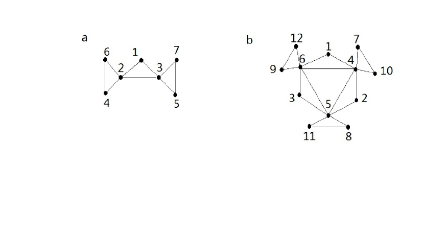
Figure 2: (a) The graph $RT(K_{2})$.    (b) The graph $RT(C_{3})$.

5.2 Cycle $C_{n}$ ($n\geq 3$)

It was reported in [23] that $Kf(C_{n})=\frac{n^{3}-n}{12}.$ It follows from Theorem 4.4 that

$$Kf(RT(C_{n}))$$

$$=\frac{(r+6)^{2}}{6}Kf(C_{n})+\frac{(r+5)n}{2}+\frac{(r+6)(5n-4)n}{6}+\frac{(r-2)(r+6)n^{2}}{8}$$

$$=\frac{(r+6)^{2}(n^{3}-n)}{72}+\frac{(r+5)n}{2}+\frac{(r+6)(5n-4)n}{6}+\frac{(r-2)(r+6)n^{2}}{8}.$$

Similarly, for graph $RT(C_{3})$, see Figure 2 (b). One can obtain

$Kf(RT(C_{3}))=\frac{455}{6},$ which also coincides with the above formula.

5.3 Complete bipartite graph $K_{n,n}$

Note that $K_{n,n}$ is $n$-regular with $2n$ vertices. Recall from [11] that

$$Kf(K_{n,n})=4n-3.$$ (35)

It follows from (14) and Theorem 4.4 that

$$Kf(RT(K_{n,n}))$$

$$=\frac{(r+6)^{2}}{6}Kf(K_{n,n})+\frac{(r+5)\cdot 2n}{2}+\frac{(r+6)(10n-4)n}{3}$$

$$~{}~{}+\frac{(r-2)(r+6)n^{2}}{2}$$

$$=\frac{(r+6)^{2}(4n-3)}{6}+(r+5)n+\frac{(r+6)(10n-4)n}{3}+\frac{(r-2)(r+6)n^{2}}{2}.$$

6 Conclusions

In this paper, based on the earlier definition $R(G)$, we introduce a novel graph operation $RT(G)$, and explore its Laplacian polynomial and Kirchhoff index. By utilizing the spectral graph theory, we establish the explicit formula for $Kf(RT(G))$ in terms of $Kf(G)$, the number of vertices and the vertex degree of regular graph $G$, based on which we propose a lower bound for the Kirchhoff index for $RT(G)$ with respect to the number of vertices and the vertex degree.

References

- [1] D. Cvetković M. Doob, H. Sachs, Spectra of Graphs-Theory and Application, Academic Press, New York, 1980.
- [2] D. J. Klein, M. Randi, Resistance distance, J. Math. Chem. 12 (1993) 81-95.
- [3] L. H. Feng, G. Yu, W. Liu, Further resuts regarding the degree Kirchhoff index of a graph, Miskolc Mathematical Notes, 151 (2014) 97-108
- [4] L. H. Feng, G. Yu, K. Xu, Z. Jiang, A note on the Kirchhoff index of bicyclic graphs, Ars Comb. 114 (2014) 33-40.
- [5] L. H. Feng, Ivan Gutman, Guihai Yu, Degree Kirchhoff index of unicyclic graphs, MATCH Commun. Math. Comput. Chem, 69 (2013) 629-648.
- [6] Y. J. Yang, D. J. Klein, A recursion formula for resistance distances and its applications, Discrete Appl. Math. 161 (2013) 2702-2715.
- [7] Y. J. Yang, D. J. Klein, Comparison theorems on resistance distances and Kirchhoff indices of S,T-isomers, Discrete Appl. Math. 175 (2014) 87-93.
- [8] Y. J. Yang, The Kirchhoff index of subdivisions of graphs, Discrete Appl. Math. 171 (2014) 153-157.
- [9] F.-Z. Zhang, The Schur Complement and its Applications, Springer, 2005.
- [10] H. Zhang, Y. Yang, C. Li, Kirchhoff index of composite graphs, Discrete Appl. Math. 157 (2009) 2918-2927.
- [11] X. Gao, Y. F. Luo, W. W. Liu, Kirchhoff index in line, subdivision and total graphs of a regular graph, Discrete Appl. Math. 160 (2012) 560-565.
- [12] W. Wang, D. Yang, Y. Luo, The Laplacian polynomial and Kirchhoff index of graphs derived from regular graphs, Discrete Appl. Math. 161 (2013) 3063-3071.
- [13] H. Y. Zhu, D. J. Klein and I. Lukovits, Extensions of the Wiener number, Journal of Chemical Information and Computer Sciences, 36 (1996) 420-428.
- [14] I. Gutman and B. Mohar, The quasi-Wiener and the Kirchhoff index coincide, Journal of Chemical Information and Computer Sciences, 36 (1996) 982-985.
- [15] B. Zhou, N. Trinajstić, A note on Kirchhoff index, Chem. Phys. Lett. 455 (2008) 120-123.
- [16] S. L. Wang, B. Zhou, The signless Laplacian spectra of the corona and edge corona of two graphs, Linear and Multilinear Algebra (2012) 1-8, iFirst.
- [17] X. Liu, P. Lu, Spectra of subdivision-vertex and subdivision-edge neighbourhood coronae, Linear Algebra Appl. 438 (2013) 3547-3559.
- [18] P. Lu, Y. Miao, Spectra of the subdivision-vertex and subdivision-edge coronae, arXiv:1302.0457.
- [19] C. McLeman, E. McNicholas, Spectra of coronae, Linear Algebra Appl. 435 (2011) 998-1007.
- [20] I. Gopalapillai, The spectrum of neighborhood corona of graphs. Kragujevac J. Math. 35 (2011) 493-500.
- [21] R. A. Horn, C. R. Johnson, Topics in Matrix Analysis, Cambridge University Press, 1991.
- [22] V. Nikiforov, The energy of graphs and matrices, J. Math. Anal. Appl. 326 (2007), 1472-1475.
- [23] I. Lukovits, S. Nikolić N. Trinajstić, Resistance distance in regular graphs, Int. J. Quantum Chem. 71 (1999) 217-225.
- [24] Z. Zhang, Some physical and chemical indices of clique-inserted lattices, Journal of Statistical Mechanics: Theory and Experiment, 10 (2013), 1-12.
- [25] J. B. Liu, X. F. Pan, J. Cao, F. F. Hu, A note on some physical and chemical indices of clique-inserted lattices , Journal of Statistical Mechanics: Theory and Experiment, 6 (2014), 1-9.