Kepler-432: a Red Giant Interacting with One of its Two Long Period Giant Planets

Abstract

We report the discovery of Kepler-432b, a giant planet (${M_{\rm b}}=5.41^{+0.32}_{-0.18}~{}{M_{\rm Jup}}$, ${R_{\rm b}}=1.145^{+0.036}_{-0.039}~{}{R_{\rm Jup}}$) transiting an evolved star ($M_{\star}=1.32^{+0.10}_{-0.07}~{}{M_{\odot}},R_{\star}=4.06^{+0.12}_{-0.08}~{}{R_{\odot}}$) with an orbital period of $P_{\rm b}=52.501129^{+0.000067}_{-0.000053}$ days. Radial velocities (RVs) reveal that Kepler-432b orbits its parent star with an eccentricity of $e=0.5134^{+0.0098}_{-0.0089}$, which we also measure independently with asterodensity profiling (AP; $e=0.507^{+0.039}_{-0.114}$), thereby confirming the validity of AP on this particular evolved star. The well determined planetary properties and unusually large mass also make this planet an important benchmark for theoretical models of super-Jupiter formation. Long-term RV monitoring detected the presence of a non-transiting outer planet (Kepler-432c; ${M_{\rm c}}\sin{i_{\rm c}}=2.43^{+0.22}_{-0.24}~{}{M_{\rm Jup}}$, $P_{\rm c}=406.2^{+3.9}_{-2.5}$ days), and adaptive optics imaging revealed a nearby ($0\farcs 87$), faint companion (Kepler-432B) that is a physically bound M dwarf. The host star exhibits high S/N asteroseismic oscillations, which enable precise measurements of the stellar mass, radius and age. Analysis of the rotational splitting of the oscillation modes additionally reveals the stellar spin axis to be nearly edge-on, which suggests that the stellar spin is likely well-aligned with the orbit of the transiting planet. Despite its long period, the obliquity of the $52.5$-day orbit may have been shaped by star–planet interaction in a manner similar to hot Jupiter systems, and we present observational and theoretical evidence to support this scenario. Finally, as a short-period outlier among giant planets orbiting giant stars, study of Kepler-432b may help explain the distribution of massive planets orbiting giant stars interior to $1$ AU.

1. Introduction

The NASA Kepler mission (Borucki et al., 2010), at its heart a statistical endeavor, has provided a rich dataset that enables ensemble studies of planetary populations, from gas giants to Earth-sized planets. Such investigations can yield valuable statistical constraints for theories of planetary formation and subsequent dynamical evolution (e.g., Buchhave et al., 2014; Steffen et al., 2012). Individual discoveries, however, provide important case studies to explore these processes in detail, especially in parameter space for which populations remain small. Because of its unprecedented photometric sensitivity, duty cycle, and time coverage, companions that are intrinsically rare or otherwise difficult to detect are expected to be found by Kepler, and detailed study of such discoveries can lead to characterization of poorly understood classes of objects and physical processes.

Planets orbiting red giants are of interest because they trace the planetary population around their progenitors, many of which are massive and can be hard to survey while they reside on the main sequence. Stars more massive than about $1.3~{}{M_{\odot}}$ (the so-called Kraft break; Kraft, 1967) have negligible convective envelopes, which prevents the generation of the magnetic winds that drive angular momentum loss in smaller stars. Their rapid rotation and high temperatures—resulting in broad spectral features that are sparse in the optical—make precise radial velocities (RVs) extremely difficult with current techniques. However, as they evolve to become giant stars, they cool and spin down, making them ideal targets for precise radial velocity work (see, e.g., Johnson et al., 2011, and references therein). There is already good evidence that planetary populations around intermediate mass stars are substantially different from those around their low mass counterparts. Higher mass stars seem to harbor more Jupiters than do Sun-like stars (Johnson et al., 2010), and the typical planetary mass correlates with the stellar mass (Lovis & Mayor, 2007; Döllinger et al., 2009; Bowler et al., 2010), but there are not many planets within $1$ AU of more massive stars (Johnson et al., 2007; Sato et al., 2008), and their orbits tend to be less eccentric than Jupiters orbiting low mass stars (Jones et al., 2014). Due to the observational difficulties associated with massive and intermediate-mass main-sequence stars, many of the more massive stars known to host planets have already reached an advanced evolutionary state, and it is not yet clear whether most of the orbital differences can be attributed to mass-dependent formation and migration, or if planetary engulfment and/or tidal evolution as the star swells on the giant branch plays a more important role.

While the number of planets known to orbit evolved stars has become substantial, because of their typically long periods, not many transit, and thus very few are amenable to detailed study. In fact, Kepler-91b (Lillo-Box et al., 2014a, b; Barclay et al., 2015) and Kepler-56c (Huber et al., 2013b) are the only two massive planets ($M_{p}>0.5~{}{M_{\rm Jup}}$) orbiting giant stars ($\log{g}<3.9$) that are known to transit. A transit leads to a radius measurement, enabling investigation of interior structure and composition via bulk density constraints and theoretical models (e.g., Fortney et al., 2007), and also opens up the possibility of atmospheric studies (e.g., Charbonneau et al., 2002; Knutson et al., 2008; Berta et al., 2012; Poppenhaeger et al., 2013), which can yield more specific details about planetary structure, weather, or atomic and molecular abundances within the atmosphere of the planet. Such information can provide additional clues about the process of planet formation around hot stars.

In studies of orbital migration of giant planets, the stellar obliquity—the angle between the stellar spin axis and the orbital angular momentum vector—has proven to be a valuable measurement, as it holds clues about the dynamical history of the planetary system (see, e.g., Albrecht et al., 2012). Assuming that the protoplanetary disk is coplanar with the stellar equator, and thus the rotational and orbital angular momenta start out well-aligned, some migration mechanisms–e.g., Type II migration (Goldreich & Tremaine, 1980; Lin & Papaloizou, 1986)—are expected to preserve low obliquities, while others—for example, Kozai cycles (e.g., Wu & Murray, 2003; Fabrycky & Tremaine, 2007), secular chaos (Wu & Lithwick, 2011), or planet-planet scattering (e.g., Rasio & Ford, 1996; Juric & Tremaine, 2008)—may excite large orbital inclinations. Measurements of stellar obliquity can thus potentially distinguish between classes of planetary migration.

The Rossiter–McLaughlin effect (McLaughlin, 1924; Rossiter, 1924) has been the main source of (projected) obliquity measurements, although at various times starspot crossings (e.g., Désert et al., 2011; Nutzman et al., 2011; Sanchis-Ojeda et al., 2011), Doppler tomography of planetary transits (e.g., Collier Cameron et al., 2010; Johnson et al., 2014), gravity-darkened models of the stellar disk during transit (e.g., Barnes et al., 2011), and the rotational splitting of asteroseismic oscillation modes (e.g., Huber et al., 2013b) have all been used to determine absolute or projected stellar obliquities. Most obliquity measurements to date have been for hot Jupiters orbiting Sun-like stars, but to get a full picture of planetary migration, we must study the dynamical histories of planets across a range of separations and in a variety of environments. Luckily, the diversity of techniques with which we can gather this information allows us to begin investigating spin–orbit misalignment for long period planets and around stars of various masses and evolutionary states. For long-period planets orbiting slowly rotating giant stars, the Rossiter–McLaughlin amplitudes are small because they scale with the stellar rotational velocity and the planet-to-star area ratio, and few transits occur, which limits the opportunities to obtain follow-up measurements or to identify the transit geometry from spot crossings. Fortunately, the detection of asteroseismic modes does not require rapid rotation, and is independent of the planetary properties, so it becomes a valuable tool for long period planets orbiting evolved stars. The high precision, high duty-cycle, long timespan, photometric observations of Kepler are ideal for both identifying long period transiting planets and examining the asteroseismic properties of their host stars.

In this paper, we highlight the discovery of Kepler-432b and c, a pair of giant planets in long period orbits ($>50$ days) around an oscillating, intermediate mass red giant. We present the photometric observations and transit light curve analysis of Kepler-432 in Section 2 and the follow-up imaging and spectroscopy in Sections 3 and 4, followed by the asteroseismic and radial velocity analyses in Sections 5 and 6. False positive scenarios and orbital stability are investigated in Sections 7 and 8, and we discuss the system in the context of planet formation and migration in Section 9, paying particular attention to star–planet interactions (SPIs) and orbital evolution during the red giant phase. We provide a summary in Section 10.

2. Photometry

2.1. Kepler Observations

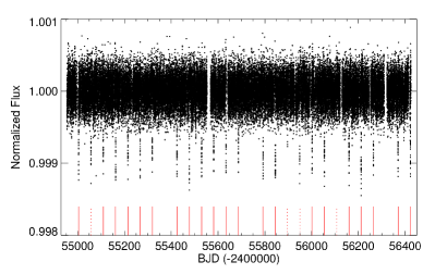
Figure 1.— Detrended and normalized long cadence Kepler time series for Kepler-432, spanning $1470.5$ days. The transits, which are clearly visible even in the unfolded data, are indicated by red lines. Solid lines denote full transits, while dotted lines denote that only a partial transit was observed. Three of the $28$ expected transits occurred entirely during data gaps.

The Kepler mission and its photometric performance are described in Borucki et al. (2010), and the characteristics of the detector on board the spacecraft are described in Koch et al. (2010) and van Cleve (2008). The photometric observations of Kepler-432 span Kepler observation Quarters 0 through 17 (JD 2454953.5 to 2456424.0), a total of $1470.5$ days. Kepler-432b was published by the Kepler team as a Kepler Object of Interest (KOI) and planetary candidate (designated KOI-1299; see Batalha et al., 2013), and after also being identified as a promising asteroseismic target, it was observed in short cadence (SC) mode for $8$ quarters. We note that a pair of recent papers have now confirmed the planetary nature of this transiting companion via radial velocity measurements (Ciceri et al., 2015; Ortiz et al., 2015).

The full photometric timeseries, normalized in each quarter, is shown in Figure 1. A transit signature with a period of $\mathord{\sim}52.5$ days is apparent in the data, and our investigation of the transits is described in the following section.

2.2. Light Curve Analysis

A transit light curve analysis of Kepler-432b was performed previously by Sliski & Kipping (2014). In that work, the authors first detrended the Simple Aperture Photometry (SAP) Kepler data for quarters $1$–$17$ using the CoFiAM (Cosine Filtering with Autocorrelation Minimization) algorithm and then regressed the cleaned data with the multimodal nested sampling algorithm MultiNest (Feroz et al., 2009) coupled to a Mandel & Agol (2002) planetary transit model. Details on the priors employed and treatment of limb darkening are described in Sliski & Kipping (2014). The authors compared the light curve derived stellar density, $\rho_{\star,\rm{obs}}$, to that from asteroseismology, $\rho_{\star,\rm{astero}}$, in a procedure dubbed “Asterodensity Profiling” (AP; Kipping et al., 2012; Kipping, 2014a) to constrain the planet’s minimum orbital eccentricity as being $e_{\rm min}=0.488_{-0.051}^{+0.025}$. The minimum eccentricity is most easily retrieved with AP but the proper eccentricity (and argument of periastron, $\omega$) can be estimated by including $e$ and $\omega$ as free parameters in the light curve fit and marginalizing over $\omega$. In order to estimate the proper eccentricity, we were motivated to re-visit the Kepler data, as described below.

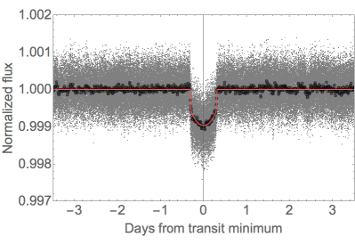
Figure 2.— Folded short cadence Kepler light curve, shown as gray points. For clarity, the binned data (every $100$ points) are overplotted as large dark circles, and the best fit, with parameters reported in Table 1, is indicated by the solid red line.

We first detrended the Kepler SAP data as was done in Sliski & Kipping (2014), by using the CoFiAM algorithm, which is described in detail in Kipping et al. (2013). CoFiAM acts like a harmonic filter, removing any long term periodicities in the data but protecting those variations occurring on the timescale of the transit or shorter, so as to retain the true light curve shape. The algorithm requires an estimate of the times of transit minimum, orbital period, and full transit duration. Since Sliski & Kipping (2014) provided refined values for these quantities, we used these updated values to conduct a revised CoFiAM detrending of the Kepler data. As with the previous analysis, the final light curves are optimized for a window within three transit durations of the transit minima.

Due to the effects of stellar granulation on the photometry, we find that the light curve scatter clearly exceeds the typical photometric uncertainties. In order to obtain more realistic parameter uncertainties, we added a “jitter” term in quadrature to the photometric uncertainties to yield a reduced chi-squared of unity for the out-of-transit data. This was done independently for the long- and short-cadence data, although the photometric jitter terms were (as expected) nearly identical at $177.4$ and $175.9\,$ppm for the short- and long-cadence data, respectively.

The $13$ long-cadence transits for which no SC data was available and the $11$ SC transits were stitched together and regressed to a transit model using MultiNest. Our light curve model employs the quadratic limb darkening Mandel & Agol (2002) routine with the Kipping (2010) “resampling” prescription for accounting for the smearing of the long-cadence data. The seven basic parameters in our light curve fit were ratio-of-radii, $R_{\rm b}/R_{\star}$, stellar density, $\rho_{\star}$, impact parameter, $b$, time of transit minimum, $T_{0}$, orbital period, $P$, and the limb darkening coefficients $q_{1}$ and $q_{2}$ described in Kipping (2013a). In addition, we included an 8th parameter for the log of the contaminated light fraction from a blend source, $\log_{10}\beta=\log_{10}(F_{\mathrm{blend}}/F_{\star})$. This was constrained from adaptive optics imaging (AO; see Section 3.2) to be $\log\beta=-2.647\pm 0.042$ with a Gaussian prior, assuming Gaussian uncertainties on the magnitudes measured from AO.

Ordinarily, a transit light curve contains very little information on the orbital eccentricity and thus it is not possible to reach a converged eccentricity solution with photometry alone (Kipping, 2008). However, in cases where the parent star’s mean density is independently constrained, a transit light curve can be used to constrain the orbital eccentricity and argument of periastron (Dawson & Johnson, 2012; Kipping, 2014a). This technique, an example of AP, enables us to include $e$ and $\omega$ as our 9th and 10th transit model parameters.

To enable the use of AP, we impose an informative Gaussian prior on the mean stellar density given by the asteroseismology constraint ($\rho_{\star,\mathrm{astero}}=27.94^{+0.55}_{-0.58}$ kg m^-3; Section 5). We use the ECCSAMPLES code (Kipping, 2014b) to draw samples from an appropriate joint $e$–$\omega$ prior. This code describes the eccentricity distribution as following a Beta distribution (a weakly informative prior) and then accounts for the bias in both $e$ and $\omega$ caused by the fact that the planet is known to transit. For the Beta distribution shape parameters, we use the “short” period calibration ($P<380$d) of Kipping (2013b): $a_{\beta}=0.697$ and $b_{\beta}=3.27$.

The maximum a posteriori folded transit light curve is presented in Figure 2. The transit parameters and associated 68.3% uncertainties, derived solely from this photometric fit, are reported in Table 1.

Table 1Kepler-432 Transit Parameters

Parameter	Value
$R_{\rm b}/R_{\star}$	$0.02914^{+0.00038}_{-0.00093}$
$\rho_{\star}~{}({\rm kg\,m}^{-3})$	$27.94^{+0.54}_{-0.58}$
$b$	$0.503^{+0.090}_{-0.168}$
$T_{\rm 0,b}$ (BJD)	$2455949.5374^{+0.0018}_{-0.0016}$
$P_{\rm b}$ (days)	$52.501134^{+0.000070}_{-0.000107}$
$q_{1}$	$0.309^{+0.047}_{-0.042}$
$q_{2}$	$0.674^{+0.151}_{-0.098}$
$\log\beta$	$-2.647\pm 0.042$
$e_{\rm b}$	$0.507^{+0.039}_{-0.114}$
$\omega_{\rm b}$ (degrees)	$76^{+59}_{-24}$

3. High Spatial Resolution Imaging

3.1. Speckle Imaging

Speckle imaging observations of Kepler-432 were performed on UT 2011 June 16 at the $3.5$ m WIYN telescope on Kitt Peak, AZ, using the Differential Speckle Survey Instrument (DSSI; Horch et al., 2010). DSSI provides simultaneous images in two filters using a dichroic beam splitter and two identical EMCCDs. These images were obtained in the $R$ ($6920$ Å) and $I$ ($8800$ Å) bands. Data reduction and analysis of these images is described in Torres et al. (2011), Horch et al. (2010), and Howell et al. (2011). The reconstructed $R$- and $I$-band images reveal no stellar companions brighter than $\Delta R\mathord{\sim}4.5$ magnitudes and $\Delta I\mathord{\sim}3.5$ magnitudes, within the annulus from $0\farcs 05$ to $2\arcsec$. The contrasts achieved as a function of distance are plotted in Figure 3, and represent $5$-$\sigma$ detection thresholds.

3.2. Adaptive Optics Imaging

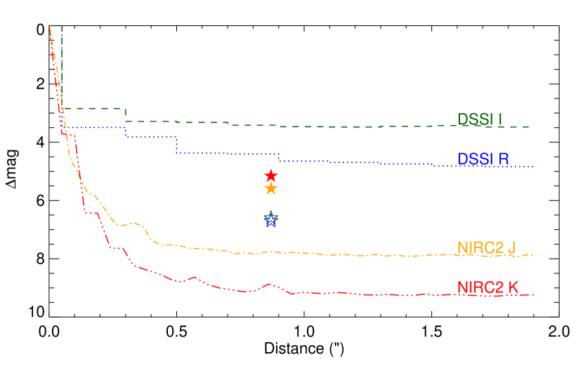
Figure 3.— Contrasts as a function of distance for all high resolution follow up, and the magnitude difference of the visual companion in each filter. Based on its infrared magnitudes from the NIRC2 $J$- and $K$-band detections (filled stars), we estimate the companion contrast in the $R$- and $I$-bands (open stars) to be $6.7$ and $6.6$ magnitudes, respectively. These magnitudes are consistent with our non-detections in the DSSI images.

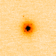
Figure 4.— NIRC2 AO images in $J$-band ($1.260~{}\micron$) and $\rm{Br}\gamma$ ($2.165~{}\micron$), $4\arcsec\!\times\!4\arcsec$ in size, with a logarithmic flux scale. A faint companion to the northeast is clearly detected in both images, with separation $0\farcs 8730\pm 0\farcs 0014$ and PA $20.86^{\circ}\pm 0.07^{\circ}$. North is up and east is left.

Adaptive optics imaging was obtained using the Near InfraRed Camera 2 (NIRC2) mounted on the Keck II $10$ m telescope on Mauna Kea, HI on UT 2014 September 4. Images were obtained in both $J$ ($1.260~{}\micron$) and Br$\gamma$ ($2.165~{}\micron$; a good proxy for both $K$ and $K_{s}$). NIRC2 has a field of view $10\arcsec\!\times\!10\arcsec$, a pixel scale of about $0\farcs 01\,{\rm pix}^{-1}$, and a rotator accuracy of $0\fdg 02$. The overlap region of the dither pattern of the observations (i.e., the size of the final combined images) is $\mathord{\sim}4\arcsec\!\times\!4\arcsec$. In both filters, the FWHM of the stellar PSF was better than $0\farcs 05$, and the achieved contrasts were $\Delta K\mathord{\sim}9$ ($\Delta J\mathord{\sim}8$) beyond $0\farcs 5$ (see Figure 3).

A visual companion was detected in both images (Figure 4) with separation $0\farcs 8730\pm 0\farcs 0014$ and PA $20\fdg 86\pm 0\fdg 07$ (east of north). Relative to Kepler-432, we calculate the companion to have magnitudes ${\Delta}J=5.59\pm 0.06$ and ${\Delta}K=5.16\pm 0.02$, implying $J-K=0.99\pm 0.07$. Using the $J-K$ colors, we estimate the magnitude in the Kepler bandpass to be $K_{\rm p}\mathord{\sim}18.8$. The object was not detected in the speckle images because they were taken with less aperture and the expected contrast ratios are larger in $R$ and $I$—using the properties of the companion as derived in the following section, we estimate $\Delta R\mathord{\sim}6.7$ and $\Delta I\mathord{\sim}6.6$. These magnitudes are consistent with non-detections in the speckle images, as plotted in Figure 3.

3.3. Properties of the Visual Companion

The faint visual companion to Kepler-432 could be a background star or a physically bound main-sequence companion. We argue that it is unlikely to be a background star, and present two pieces of evidence to support this conclusion. We first estimate the background stellar density in the direction of Kepler-432 using the TRILEGAL stellar population synthesis tool (Girardi et al., 2005): we expect $49,\!000$ sources per deg² that are brighter than $K_{s}\mathord{\sim}19$ (the detection limit of our observation). This translates to $0.06$ sources (of any brightness and color) expected in our $16~{}{\rm arcsec}^{2}$ image, and thus the a priori probability of a chance alignment is low.

Furthermore, since we know the properties of the primary star, we can determine whether there exists a coeval main-sequence star that could adequately produce the observed colors and magnitude differences. Using the asteroseismically derived mass, radius, and age of the primary (see Section 5), we place the primary star on an appropriate Padova PARSEC isochrone (Bressan et al., 2012; Chen et al., 2014). We then use the observed magnitude differences between the stars to search for an appropriate match to the companion in the isochrone. If the visual companion is actually a background giant, it is unlikely that it would happen to be at the right distance to match both the colors and brightness of a physically bound companion. Therefore, we do not expect a background giant star to lie on the isochrone. However, we do find a close match to the observed colors and magnitudes of the companion (see Figure 5), further suggesting that it is not a background object, but truly a physical companion, and this allows us to estimate its properties from the isochrone.

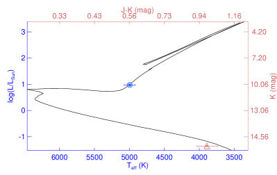
Figure 5.— Kepler-432 (blue circle) placed on a $3.5$ Gyr, ${\rm[m/H]=-0.07}$ PARSEC isochrone (Bressan et al., 2012), plotted as a solid black line. The upper right (red) axes represent the $J-K$ and apparent $K$ mag corresponding to the $T_{\rm eff}$ and $\log{L/L\odot}$ on the lower left (blue) axes. The visual companion (red triangle) is placed on the plot according to its measured $J-K$ and $K$ mag. It lies very near the isochrone for the system, suggesting that it is indeed coeval with and physically bound to Kepler-432, rather than a background star.

We conclude that the companion is most likely a physically bound, coeval M dwarf with a mass of $\mathord{\sim}0.52~{}{M_{\odot}}$ and an effective temperature of $\mathord{\sim}3660$ K. The distance to the system ($\mathord{\sim}870$ pc; Section 5.5), implies that the projected separation of the companion is $\mathord{\sim}750$ AU. Using this as an estimate of the semi-major axis, the binary orbital period is on the order of $15,\!000$ yr. In reality, the semi-major axis may be smaller (if we observed it near apastron of an eccentric orbit with the major axis in the plane of the sky), or significantly larger (due to projections into the plane of the sky and the unknown orbital phase).

We discuss the possibility of false positives due to this previously undetected companion in Section 7.

4. Spectroscopic Follow-Up

4.1. Spectroscopic Observations

We used the Tillinghast Reflector Echelle Spectrograph (TRES; Fűrész, 2008) mounted on the $1.5$-m Tillinghast Reflector at the Fred L. Whipple Observatory (FLWO) on Mt. Hopkins, AZ to obtain $84$ high resolution spectra of Kepler-432 between UT 2011 March 23 and 2014 June 18. TRES is a temperature-controlled, fiber-fed instrument with a resolving power of $R\mathord{\sim}44,\!000$ and a wavelength coverage of $\mathord{\sim}3850$–$9100$ Å, spanning $51$ echelle orders. Typical exposure times were $15$-$30$ minutes, and resulted in extracted signal-to-noise ratios (S/Ns) between about $20$ and $45$ per resolution element. The goal of the intial observations was to rule out false positives involving stellar binaries as part of the Kepler Follow-up Observing Program (KFOP, which has evolved into CFOP), but upon analysis of the first few spectra, it became clear that the planet was massive enough to confirm with an instrument like TRES that has a modest aperture and $\mathord{\sim}10~{}{\rm m\thinspace s^{-1}}$ precision (see, e.g., Quinn et al., 2014). By the second observing season, an additional velocity trend was observed, which led to an extended campaign of observations.

Precise wavelength calibration of the spectra was established by obtaining ThAr emission-line spectra before and after each spectrum, through the same fiber as the science exposures. Nightly observations of the IAU RV standard star HD 182488 helped us track the achieved instrumental precision and correct for any RV zero point drift. We also shift the absolute velocities from each run so that the median RV of HD 182488 is $-21.508~{}{\rm km\thinspace s^{-1}}$ (Nidever et al., 2002). This allows us to report the absolute systemic velocity, $\gamma_{\rm abs}$. We are aware of specific TRES hardware malfunctions (and upgrades) that occurred during the timespan of our data that, in addition to small zero point shifts (typically $<10{\rm m\thinspace s^{-1}}$), caused degradation (or improvement) of RV precision for particular observing runs. For example, the installation of a new dewar lens caused a zero point shift after BJD 2455750, and a second shift (accompanied by significant improvement in precision) occurred when the fiber positioner was fixed in place on BJD 2456013. It will be important to treat these with care so that the radial velocities are accurate and each receives its appropriate weight in our analysis.

We also obtained five spectra with the FIber-fed Echelle Spectrograph (FIES; Frandsen & Lindberg, 1999) on the $2.5$-m Nordic Optical Telescope (NOT; Djupvik & Andersen, 2010) at La Palma, Spain during the first observing season (UT 2011 August 4 through 2011 October 7) to confirm the initial RV detection before continuing to monitor the star with TRES. Like TRES, FIES is a temperature-controlled, fiber-fed instrument, and has a resolving power through the medium fiber of ${\rm R}\mathord{\sim}46,\!000$, a wavelength coverage of $\mathord{\sim}3600$–$7400$ Å, and wavelength calibration determined from ThAr emission-line spectra.

4.2. Spectroscopic Reduction and Radial Velocity Determination

We will discuss the reduction of spectra from both instruments collectively but only briefly (more details can be found in Buchhave et al., 2010) while detailing the challenges presented by our particular data set. Spectra were optimally extracted, rectified to intensity versus wavelength, and cross-correlated, order by order, using the strongest exposure as a template. We used $21$ orders (spanning $4290$–$6280$ Å), rejecting those plagued by telluric lines, fringing in the red, and low S/N in the blue. For each epoch, the cross-correlation functions (CCFs) from all orders were added and fit with a Gaussian to determine the relative RV for that epoch. Using the summed CCF rather than the mean of RVs from each order naturally weights the orders with high correlation coefficients more strongly. Internal error estimates for each observation were calculated as $\sigma_{\rm int}={\rm rms}(\vec{v})/\sqrt{N}$, where $\vec{v}$ is the RV of each order, $N$ is the number of orders, and rms denotes the root mean squared velocity difference from the mean. These internal errors account for photon noise and the precision with which we can measure the line centers, which in turn depends on the characteristics of the Kepler-432 spectrum (line shapes, number of lines, etc), but do not account for errors introduced by the instrument itself.

The nightly observations of RV standards were used to correct for systematic velocity shifts between runs and to estimate the instrumental precision. The median RV of HD 182488 was calculated for each run, which we applied as shifts to the Kepler-432 velocities, keeping in mind that each shift introduces additional uncertainty. By also applying the run-to-run offsets to the standard star RVs themselves, we were able to evaluate the residual RV noise introduced by the limited instrumental precision (separate from systematic zero point shifts). After correction, the rms of the standard star RVs in each run was consistent with the internal errors. This indicates that the additional uncertainty introduced by run-to-run correction already adequately accounts for the instrumental uncertainty, and we do not need to explicitly include an additional error term to account for it. The final error budget of Kepler-432 RVs was assumed to be the sum by quadrature of all RV error sources—internal errors, run-to-run offset uncertainties, and TRES instrumental precision: $\sigma_{\rm RV}^{2}=\sigma_{\rm int}^{2}+\sigma_{\rm run}^{2}+\sigma_{\rm TRES}^{2}$, where the final term $\sigma_{\rm TRES}=0$ because it is implicitly incorporated into $\sigma_{\rm run}$. The final radial velocities are listed in Table 2. We recognize that stellar jitter or additional undetected planets may also act as noise sources, and we address this during the orbital fitting analysis in Section 6.

Table 2Kepler-432 Relative Radial Velocities

BJD	$v$	$\sigma_{v}$	BJD	$v$	$\sigma_{v}$
(-2455000)	(m s-1)	(m s-1)	(-2455000)	(m s-1)	(m s-1)
$644.00217$	$235.4$	$65.1$	$1083.87676$	$338.7$	$36.7$
$722.95848$	$453.1$	$23.0$	$1091.93504$	$489.2$	$44.3$
$727.87487$	$452.2$	$72.1$	$1117.90004$	$211.7$	$41.6$
$734.86675$	$544.4$	$68.2$	$1132.79275$	$410.9$	$42.4$
$755.93317$	$47.2$	$18.9$	$1137.83647$	$333.7$	$21.8$
$757.82852$	$197.1$	$23.7$	$1175.82536$	$210.1$	$62.5$
$758.88922$	$121.7$	$18.9$	$1197.74504$	$394.7$	$22.3$
$760.95496$	$193.8$	$25.9$	$1202.70980$	$495.3$	$20.5$
$764.92787$	$270.3$	$36.7$	$1227.64276$	$75.4$	$23.1$
$768.78698$	$262.1$	$33.9$	$1233.59012$	$213.1$	$32.0$
$768.80782$	$277.4$	$30.8$	$1258.59157$	$564.4$	$24.3$
$822.70873$	$197.0$	$54.9$	$1279.58992$	$96.6$	$28.9$
$825.63058$	$265.0$	$53.1$	$1376.99835$	$29.1$	$25.1$
$826.64436$	$310.1$	$53.0$	$1382.93180$	$148.7$	$23.9$
$827.71851$	$362.0$	$55.3$	$1389.91148$	$179.3$	$26.7$
$828.61567$	$358.8$	$60.8$	$1400.93674$	$384.5$	$31.0$
$829.72558$	$358.7$	$53.9$	$1405.90249$	$465.6$	$30.5$
$830.69401$	$446.6$	$56.2$	$1409.87680$	$507.5$	$28.4$
$837.59392$	$588.0$	$51.1$	$1413.96428$	$646.1$	$37.2$
$840.65649$	$603.7$	$51.0$	$1429.95861$	$111.4$	$23.7$
$841.70196$	$706.7$	$71.9$	$1436.83822$	$153.9$	$22.7$
$842.57863$	$574.4$	$57.1$	$1442.84894$	$191.6$	$26.9$
$843.59367$	$437.4$	$43.8$	$1446.78723$	$285.9$	$21.2$
$844.64075$	$346.9$	$46.7$	$1503.72052$	$351.9$	$35.0$
$845.68516$	$157.7$	$45.8$	$1547.69956$	$189.1$	$19.5$
$846.62110$	$91.9$	$45.3$	$1551.63468$	$217.2$	$20.0$
$852.61538$	$64.2$	$47.3$	$1556.67843$	$292.6$	$20.9$
$854.62438$	$57.6$	$48.9$	$1561.63231$	$370.3$	$18.2$
$856.71790$	$132.6$	$56.1$	$1575.69266$	$593.5$	$20.0$
$858.64825$	$105.2$	$48.9$	$1581.66560$	$141.4$	$18.9$
$1027.94566$	$284.4$	$26.4$	$1586.63377$	$40.5$	$18.4$
$1046.89934$	$594.1$	$20.6$	$1591.70580$	$100.0$	$21.4$
$1047.87727$	$702.8$	$38.6$	$1729.01428$	$553.2$	$37.9$
$1048.86080$	$693.7$	$18.9$	$1740.94781$	$98.6$	$33.0$
$1049.97884$	$661.7$	$28.7$	$1743.99496$	$34.8$	$29.3$
$1051.99004$	$631.1$	$24.6$	$1799.87657$	$37.0$	$26.3$
$1052.93268$	$583.1$	$30.0$	$1816.87894$	$248.9$	$32.0$
$1053.90973$	$461.0$	$23.4$	$1822.88725$	$364.1$	$24.3$
$1054.88376$	$383.9$	$29.3$	$1826.79500$	$419.8$	$20.0$
$1055.88175$	$282.3$	$37.3$	$777.59554$	$-100.9$	$10.7$
$1056.88078$	$239.3$	$26.4$	$778.59121$	$-81.1$	$10.5$
$1057.95303$	$158.7$	$24.6$	$779.59677$	$-51.2$	$14.1$
$1058.84781$	$160.9$	$33.7$	$782.57231$	$0.0$	$10.2$
$1074.90585$	$267.8$	$31.1$	$842.41733$	$47.7$	$10.2$
$1080.95245$	$354.5$	$30.6$

4.3. Spectroscopic Classification

Table 3Stellar Properties of Kepler-432

Parameter	Value
Asteroseismic	Grid-based Modeling	Frequency Modeling
$\Delta\nu$ ($\mu\rm{Hz}$)	$18.59\pm 0.04$	…
$\nu_{\rm max}$ ($\mu\rm{Hz}$)	$266\pm 3$	…
$\log(g)$ (dex)	$3.340\pm 0.006$	$3.345\pm 0.006$
$\rho_{\star}$ (${\rm g~{}cm}^{-3}$)	$0.02723^{+0.00054}_{-0.00057}$	$0.02794^{+0.00055}_{-0.00058}$
$R$ ($R_{\odot}$)	$4.12^{+0.12}_{-0.08}$	$4.06^{+0.12}_{-0.08}$
$M$ ($M_{\odot}$)	$1.35^{+0.10}_{-0.07}$	$1.32^{+0.10}_{-0.07}$
Age (Gyr)	$3.5^{+0.7}_{-0.8}$	$4.2^{+0.8}_{-1.0}$
Spectroscopic
$T_{\rm eff}$ (K)	$4995\pm 78$
$\log{g}$ (cgs)	$3.345\pm 0.006$
$[m/H]$	$-0.07\pm 0.10$
$v\sin{i_{\star}}$ (km s-1)	$2.7\pm 0.5$
Photometric
$V$ (mag)	$12.465\pm 0.060$
$K_{\rm p}$ (mag)	$12.183\pm 0.020$
$J$ (mag)	$10.684\pm 0.021$
$H$ (mag)	$10.221\pm 0.019$
$K_{\rm s}$ (mag)	$10.121\pm 0.017$
Derived
$L_{\star}$ ($L_{\odot}$)	$9.206\pm 0.010$
$d$ (pc)	$870\pm 20$
$i_{\star}$ (∘)	$90^{+0}_{-8}$
$P_{\rm rot}$ (days)	$77\pm 14$

Note. — While we have separated the stellar properties by observational technique, many of them are interdependent, for example, as described in Sections 4 and 5. We adopt the asteroseismic results from detailed frequency modeling (rather than the grid-based approach) in subsequent analyses.

We initially determined the spectroscopic stellar properties (effective temperature, $T_{\rm eff}$; surface gravity, $\log{g}$; projected rotational velocity, $v\sin{i}$; and metallicity, [m/H]) using Stellar Parameter Classification (SPC; Buchhave et al., 2012), with the goal of providing an accurate temperature for the asteroseismic modeling (see Section 5). SPC cross-correlates an observed spectrum against a grid of synthetic spectra, and uses the correlation peak heights to fit a three-dimensional surface in order to find the best combination of atmospheric parameters ($v\sin{i}$ is fit iteratively since it only weakly correlates with the other parameters). We used the CfA library of synthetic spectra, which are based on Kurucz model atmospheres (Kurucz, 1992). SPC, like other spectroscopic classifications, can be limited by degeneracy between $T_{\rm eff}$, $\log{g}$, and [m/H] (see a discussion in Torres et al., 2012), but asteroseismology provides a nearly independent measure of the surface gravity (depending only weakly on the effective temperature and metallicity). This allows one to iterate the two analyses until agreement is reached, generally requiring only $1$ iteration (see, e.g., Huber et al., 2013a). In our initial analysis, we found $T_{\rm eff}=5072\pm 55$ K, $\log{g}=3.49\pm 0.11$, ${\rm[m/H]}=-0.02\pm 0.08$, and $v\sin{i}=2.5\pm 0.5~{}{\rm km\thinspace s^{-1}}$. After iterating with the asteroseismic analysis and fixing the final asteroseismic gravity, we find similar values: $T_{\rm eff}=4995\pm 78$ K, $\log{g}=3.345\pm 0.006$, ${\rm[m/H]}=-0.07\pm 0.10$, and $v\sin{i}=2.7\pm 0.5~{}{\rm km\thinspace s^{-1}}$. We adopt the values from the combined analysis, and these final spectroscopic parameters are listed in Table 3.

5. Asteroseismology of Kepler-432

5.1. Background

Cool stars exhibit brightness variations due to oscillations driven by near-surface convection (Houdek et al., 1999; Aerts et al., 2010), which are a powerful tool to study their density profiles and evolutionary states. A simple asteroseismic analysis is based on the average separation of modes of equal spherical degree ($\Delta\nu$) and the frequency of maximum oscillation power ($\nu_{\rm max}$), using scaling relations to estimate the mean stellar density, surface gravity, radius, and mass (Kjeldsen & Bedding, 1995; Stello et al., 2008; Kallinger et al., 2010; Belkacem et al., 2011). Huber et al. (2013a) presented an asteroseismic analysis of Kepler-432 by measuring $\Delta\nu$ and $\nu_{\rm max}$ using three quarters of SC data, combined with an SPC analysis (Buchhave et al., 2012) of high-resolution spectra obtained with the FIES and TRES spectrographs. The results showed that Kepler-432 is an evolved star just beginning to ascend the red-giant branch (RGB), with a radius of $R=4.16\pm 0.12$ $R_{\odot}$ and a mass of $1.35\pm 0.10$ $M_{\odot}$ (Table 3, Figure 5).

Compared to average oscillation properties, individual frequencies offer a greatly increased amount of information by probing the interior sound speed profile. In particular, evolved stars oscillate in mixed modes, which occur when pressure modes excited on the surface couple with gravity modes confined to the core (Aizenman et al., 1977). Mixed modes place tight constraints on fundamental properties such as stellar age, and provide the possibility to probe the core structure and rotation (Bedding et al., 2011; Beck et al., 2012; Mosser et al., 2012a). Importantly, relative amplitudes of individual oscillation modes that are split by rotation can be used to infer the stellar line-of-sight inclination (Gizon & Solanki, 2003), providing valuable information on the orbital architectures of transiting exoplanet systems (e.g., Chaplin et al., 2013; Huber et al., 2013b; Benomar et al., 2014; Lund et al., 2014; Van Eylen et al., 2014). In the following section we expand on the initial asteroseismic analysis by Huber et al. (2013a) by performing a detailed individual frequency analysis based on all eight quarters (Q9–17) of Kepler short-cadence data.

5.2. Frequency Analysis

The time series was prepared for asteroseismic analysis from the raw Kepler target pixel data using the Kepler Asteroseismic Science Operations Center (KASOC) filter (Handberg & Lund, 2014). The KASOC filter removes instrumental and transit signals from the light curve, which may produce spurious peaks in the frequency domain. The power spectrum, shown in Figure 6, was computed using a Lomb–Scargle periodogram (Lomb, 1976; Scargle, 1982) calibrated to satisfy Parseval’s theorem.

The pattern of oscillation modes in the power spectrum is typical of red giants, with $\ell=0$ modes of consecutive order being approximately equally spaced by $\Delta\nu$, adjacent to $\ell=2$ modes. In addition to the $\ell=0,2$ pairs, several $\ell=1$ mixed modes are observed in each radial order which, on inspection, are the outer components of rotationally split triplets corresponding to the $m=\pm 1$ modes. This indicates that the star is seen equator-on (see Section 5.3).

The relative $p$- and $g$-mode behavior of each mixed mode depends on the strength of the coupling between the oscillation cavities in the stellar core and envelope. Detecting the $\ell=1$ modes with the greatest $g$-mode character may be challenging because they have low amplitudes, and overlap in frequency with the $\ell=0$ and $\ell=2$ modes. Adding to the possible confusion, mixed $\ell=2$ and $\ell=3$ modes may also be present, although the weaker coupling between the $p$- and $g$-modes results in only the most $p$-like modes having an observable amplitude.

Table 4Oscillation Frequencies of Kepler-432

Order	$\ell=0$	$\ell=1$		$\ell=2$	$\ell=3$
		$m=0$	$\nu_{s}$
9	$194.111^{+0.018}_{-0.014}$	$202.500^{+0.006}_{-0.008}$	$0.184^{+0.014}_{-0.013}$	$209.990^{+0.010}_{-0.023}$
		$204.392^{+0.015}_{-0.010}$	$0.274^{+0.018}_{-0.022}$
		$207.713^{+0.006}_{-0.007}$	$0.335^{+0.009}_{-0.008}$
10	$212.214^{+0.026}_{-0.020}$	$215.394^{+0.008}_{-0.007}$	$0.342^{+0.014}_{-0.015}$	$228.236^{+0.019}_{-0.019}$
		$219.215^{+0.006}_{-0.008}$	$0.284^{+0.007}_{-0.008}$
		$221.586^{+0.011}_{-0.019}$	$0.165^{+0.014}_{-0.011}$
		$224.590^{+0.016}_{-0.008}$	$0.325^{+0.017}_{-0.017}$
		$228.905^{+0.020}_{-0.013}$	$0.328^{+0.022}_{-0.017}$
11	$230.704^{+0.009}_{-0.008}$	$233.410^{+0.013}_{-0.017}$	$0.280^{+0.015}_{-0.018}$	$247.031^{+0.013}_{-0.016}$	$253.534^{+0.018}_{-0.034}$
		$237.904^{+0.014}_{-0.011}$	$0.279^{+0.010}_{-0.010}$
		$240.439^{+0.011}_{-0.009}$	$0.169^{+0.008}_{-0.009}$
		$244.157^{+0.015}_{-0.009}$	$0.302^{+0.009}_{-0.019}$
12	$249.259^{+0.016}_{-0.009}$	$254.553^{+0.005}_{-0.006}$	$0.313^{+0.005}_{-0.005}$	$265.636^{+0.011}_{-0.043}$	$272.212^{+0.015}_{-0.006}$
		$258.288^{+0.006}_{-0.008}$	$0.143^{+0.010}_{-0.011}$
		$261.490^{+0.003}_{-0.004}$	$0.298^{+0.005}_{-0.006}$
13	$267.757^{+0.017}_{-0.016}$	$273.216^{+0.007}_{-0.007}$	$0.301^{+0.007}_{-0.007}$	$284.389^{+0.013}_{-0.011}$	$291.410^{+0.008}_{-0.008}$
		$277.110^{+0.006}_{-0.008}$	$0.140^{+0.012}_{-0.014}$
		$281.091^{+0.006}_{-0.006}$	$0.304^{+0.007}_{-0.008}$
14	$286.457^{+0.006}_{-0.009}$	$294.131^{+0.015}_{-0.014}$	$0.246^{+0.012}_{-0.011}$	$303.352^{+0.021}_{-0.015}$
		$297.229^{+0.012}_{-0.017}$	$0.173^{+0.016}_{-0.014}$
15	$305.284^{+0.015}_{-0.014}$	$315.134^{+0.032}_{-0.011}$	$0.207^{+0.026}_{-0.026}$

Note. — All frequencies are in units of $\mu\rm{Hz}$. The $\ell=1$ modes are presented as the central frequency of the rotationally split mode profile ($m=0$), along with the value of the rotational splitting between the $m=0$ and $m=\pm 1$ components, $\nu_{s}$.

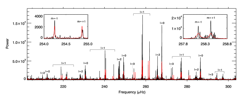
Figure 6.— Power spectrum of Kepler-432. The red curve shows the fit to the power spectrum. Insets show a close-up of two rotationally split $\ell=1$ mixed modes. The left inset shows a mixed mode dominated by $g$-mode characteristics, with lower amplitudes, narrower linewidths and a larger rotational splitting relative to the mixed mode on the right, which has strong $p$-mode characteristics.

The first step to fitting the oscillation modes and extracting their frequencies is to correctly identify the modes present. Fortunately, the $\ell=1$ mixed modes follow a frequency pattern that arises from coupling of the $p$-modes in the envelope, which have approximately equal spacing in frequency ($\Delta\nu$), to $g$-modes in the core, which are approximately equally spaced in period ($\Delta\Pi$). This pattern is well described by the asymptotic relation for mixed modes (Mosser et al., 2012b). We calculated the asymptotic mixed mode frequencies by fitting this relation to several of the highest-amplitude $\ell=1$ modes. From these calculations, nearby peaks could be associated with $\ell=1$ mixed modes. In this way we have been able to identify both of the $m=\pm 1$ components for 21 out of 27 $\ell=1$ mixed modes between $200$ and $320$ $\mu\rm{Hz}$.

Following a strategy that has been implemented in the mode fitting of other Kepler stars (e.g., Appourchaux et al., 2012), three teams performed fits to the identified modes. The mode frequencies from each fit were compared to the mean values, and the fitter that differed least overall was selected to provide the frequency solution. This fitter performed a final fit to the power spectrum to include modes that other fitters had detected, but were absent from this fitter’s initial solution.

The final fit was made using a Markov chain Monte Carlo (MCMC) method that performs a global fit to the oscillation spectrum, with the modes modeled as Lorentzian profiles (Handberg & Campante, 2011). Each $\ell=1$ triplet was modeled with the frequency splitting and inclination angle as additional parameters to the usual frequency, height, and width that define a single Lorentzian profile. Owing to the differing sensitivity of the $\ell=1$ mixed modes to rotation at different depths within the star, each $\ell=1$ triplet was fitted with an independent frequency splitting, although a common inclination angle was used. We discuss the rotation of the star further in Section 5.3.

The measured mode frequencies are given in Table 4. The values of the $\ell=1$ modes are presented as the central frequency of the rotationally split mode profile, which corresponds to the value of the $m=0$ component, along with the value of the rotational splitting between the $m=0$ and $m=\pm 1$ components, $\nu_{s}$. Revised values of $\Delta\nu$ and $\nu_{\rm max}$ can be obtained from the measured mode frequencies and amplitudes. We find $\Delta\nu$ $=~{}18.59\pm 0.04$ $\mu\rm{Hz}$ and $\nu_{\rm max}$ $=~{}266\pm 3$ $\mu\rm{Hz}$, both of which are in agreement with the values provided by Huber et al. (2013a). Additionally, we measure the underlying $\ell=1$ $g$-mode period spacing, $\Delta\Pi_{1}$, to be $89.9\pm 0.3$ s, which is consistent with a red giant branch star with a mass below $\sim 1.6\,$$M_{\odot}$ (e.g., Stello et al., 2013).

5.3. Host Star Inclination

The line-of-sight inclination of a rotating star can be determined by measuring the relative heights of rotationally split modes (Gizon & Solanki, 2003). A star viewed pole-on produces no visible splitting, while stars viewed with an inclination near $i=45^{\circ}$ would produce a frequency triplet. Figure 6 shows that all dipole modes observed for Kepler-432 are split into doublets, which we interpret as triplets with the central peak missing, indicating a rotation axis nearly perpendicular to the line of sight (inclination $i=90^{\circ}$).

To measure the inclination of Kepler-432, we included rotationally split Lorentzian profiles for each of the 21 dipole modes in the global MCMC fit of the power spectrum. Figure 7 shows the posterior distribution of the stellar inclination. The mode of the posterior distribution and $68.3\%$ highest probability density region is $90.0^{+0.0}_{-3.7}$ deg.

The inclination estimate is based on three important assumptions: the inclination is the same for $p$-dominated and $g$-dominated mixed modes, that there is equipartition of energy between modes with the same $n$ and $\ell$, and that the modes are well-resolved.

To test the first assumption, we performed additional fits to individual $\ell=1$ modes using the Python implementaiton of the nested sampling algorithm MultiNest, pyMultiNest (Feroz et al., 2013; Buchner et al., 2014). No significant difference was found between the inclination angle for $p$-dominated and $g$-dominated mixed modes. We therefore use the results of our global MCMC fit. Huber et al. (2013b) similarly found no difference between the inclination angle of $p$-dominated and $g$-dominated mixed modes in Kepler-56. Beck et al. (2014) have shown that these modes actually have slightly different pulsation cavities. They identified asymmetric rotational splittings between $m=0$ and $m=\pm 1$ modes in the red giant KIC 5006817, which results from the modes having varying $p$- and $g$-mode characteristics. Besides the effect on the rotational splitting, there is also a small impact on mode heights and lifetimes. Beck et al. (2014) further note that the asymmetries are mirrored about the frequency of the uncoupled $p$-modes. This means that the heights of the $m=\pm 1$ components relative to the $m=0$ component will change in opposite directions, so the effect can be mitigated by forcing the $m=\pm 1$ components to have the same height in the fit, as well as by performing a global fit to all modes, as we have done.

Unless mode lifetimes are much shorter than the observing baseline, the Lorentzian profiles of the modes will not be well-resolved, and the mode heights will vary. We determined the effect on the measured inclination angle in the manner of Huber et al. (2013b), by investigating the impact on simulated data with similar properties to the frequency spectrum of Kepler-432. Taking this effect into account in the determination of our measurement uncertainty, we find a final value of $i=90^{+0}_{-8}$ deg. The asteroseismic analysis therefore shows directly that the spin axis of the host star is in the plane of the sky.

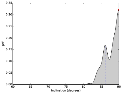
Figure 7.— Posterior of the host star line-of-sight inclination derived from the MCMC analysis of the oscillation power spectrum of Kepler-432. The red point indicates the mode of the distribution, and the blue dashed line indicates the limit of the 68% highest probability density region.

5.4. Modeling

Two approaches may be used when performing asteroseismic modeling. The first is the so-called grid-based method, which uses evolutionary tracks that cover a wide range of metallicities and masses, and searches for the best fitting model using $\Delta\nu$, $\nu_{\rm max}$, $T_{\rm eff}$, and $\rm{[Fe/H]}$ as constraints (e.g. Stello et al., 2009; Basu et al., 2010; Gai et al., 2011; Chaplin et al., 2014). The second is detailed frequency modeling, which uses individual mode frequencies instead of the global asteroseismic parameters to more precisely determine the best-fitting model (e.g., Metcalfe et al., 2010; Jiang et al., 2011). For comparison, we have modeled Kepler-432 using both approaches.

For the grid-based method we used the Garching Stellar Evolution Code (Weiss & Schlattl, 2008). The detailed parameters of this grid are described by Silva Aguirre et al. (2012) and its coverage has been now extended to stars evolved in the RGB phase. The spectroscopic values of $T_{\rm eff}$ and $\rm{[Fe/H]}$ found in Section 4.3, and our new asteroseismic measurements of $\Delta\nu$ and $\nu_{\rm max}$ were used as inputs in a Bayesian scheme as described in Silva Aguirre et al. (2014). Note that while [Fe/H] is the model input, our spectroscopic analysis yields an estimate of [m/H]. We have assumed that the two are equivalent for Kepler-432 (i.e., that the star has a scaled solar composition). If this assumption is invalid, it may introduce a small bias in our results, which are given in Table 3. The values of mass and radius agree well with those from Huber et al. (2013a), who also used the grid-based method. We note that a comparison of results provided by several grid-pipelines by Chaplin et al. (2014) found typical systematic uncertainties of $3.7\%$ in mass, $1.3\%$ in radius, and $12\%$ in age across an ensemble of main-sequence and subgiant stars with spectroscopic constraints on $T_{\rm eff}$ and $\rm{[Fe/H]}$.

We performed two detailed modeling analyses using separate stellar evolution codes in order to better account for systematic uncertainties. The first analysis modeled the star using the integrated astero extension within MESA (Paxton et al., 2013). After an initial grid search to determine the approximate location of the the global minimum, we found the best-fitting model using the build-in simplex minimization routine, which automatically adjusted the mass, metallicity, and the mixing length parameter. The theoretical frequencies were calculated using GYRE (Townsend & Teitler, 2013) and were corrected for near-surface effects using the power-law correction of Kjeldsen et al. (2008) for radial modes. The non-radial modes in red giants are mixed with $g$-mode characteristics in the core, so they are less affected by near-surface effects. To account for this, MESA-astero follows Brandão et al. (2011) in scaling the correction term for non-radial modes by $Q_{n,\ell}^{-1}$, where $Q_{n,\ell}$ is the ratio of the inertia of the mode to the inertia of a radial mode at the same frequency.

The second analysis was performed with the Aarhus Stellar Evolution Code (ASTEC; Christensen-Dalsgaard, 2008a), with theoretical frequencies calculated using the Aarhus adiabatic oscillation package (Christensen-Dalsgaard, 2008b). The best-fitting model was found in a similar manner as the first analysis, although the mixing length parameter was kept fixed at a value of $\alpha=1.8$.

Figure 8 shows the best-fitting models compared to the observed frequencies in an échelle diagram. Both analyses found an asteroseismic mass and radius of $M=1.32^{+0.10}_{-0.07}$ $M_{\odot}$and $R=4.06^{+0.12}_{-0.08}$ $R_{\odot}$, but differ in the value of the age, with the best-fitting MESA and ASTEC models having ages of $4.2^{+0.8}_{-1.0}$ and $2.9^{+0.6}_{-0.7}$ Gyr, respectively. Uncertainties were estimated by adopting the fractional uncertainties of the grid-based method, thereby accounting for systematic uncertainties in model input physics and treatment of near-surface effects. The consistency between the detailed model fitting results and grid-based results demonstrates the precise stellar characterization that can be provided by asteroseismology. Throughout the remainder of the paper we adopt the results obtained with the MESA code, though we use an age of $3.5$ Gyr, which is consistent with both detailed frequency analyses as well as the age from the grid-based modeling.

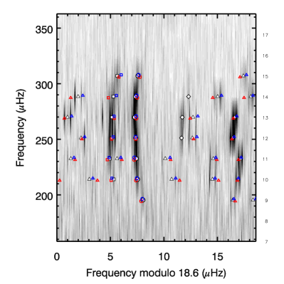
Figure 8.— Échelle diagram of Kepler-432 showing observed frequencies in white. Modes are identified as $\ell=0$ (circles), $\ell=1$ (triangles), $\ell=2$ (squares) and $\ell=3$ (diamonds). Frequencies of the best-fitting MESA and ASTEC models are indicated by the red and blue open symbols, respectively. For reference, a gray-scale map of the power spectrum is shown in the background. Numbers to the right of the plot indicate the radial order of the $\ell=0$ modes.

5.5. Distance and Reddening

The stellar model best-fit to the derived stellar properties provides color indices that may be compared against measured values as a consistency check, and as a means to determine a photometric distance to the system. Given the physical stellar parameters derived from the asteroseismic and spectroscopic measurements, the PARSEC isochrones (Bressan et al., 2012) predict $J-K_{\rm s}=0.564$, in good agreement with the measured 2MASS colors ($J-K_{\rm s}=0.563\pm 0.028$). While this indicates the dust extinction along the line of sight is probably low, we attempt to correct for it nonetheless using galactic dust maps. The mean of the reddening values reported by Schlafly & Finkbeiner (2011) and Schlegel et al. (1998)—$E(B-V)=0.079\pm 0.008$—is indeed low, implying extinction in the infrared of ${\rm A_{J}}=0.070$, ${\rm A_{H}}=0.045$, and ${\rm A_{K_{s}}}=0.028$. Applying these corrections, the observed 2MASS index becomes $J-K_{\rm s}=0.521$, now slightly inconsistent at the $1$-$\sigma$ level with the PARSEC model colors. We note that if only a small fraction of the dust column lies between us and Kepler-432, it would lead to a slight over-correction of the magnitudes and distance. The distances derived in the two cases (using $J,H,{\rm and}~{}K_{s}$ magnitudes) are $878\pm 9$ pc (no extinction) and $859\pm 13$ pc (entire column of extinction). Because the colors agree more closely without an extinction correction, it is tempting to conclude that only a small fraction of the extinction in the direction of Kepler-432 actually lies between us and the star. However, in the direction to the star (i.e., out of the galactic plane), it seems unlikely that a significant column of absorbers would lie beyond $\mathord{\sim}1$ kpc. In reality, the model magnitudes are probably not a perfect match for the star and the appropriate reddening for this star is probably between $0$ and that implied by the full column ($0.079$). The derived distance does not depend strongly on the value we adopt for reddening, and we choose to use the mean of the two distance estimates and slightly inflate the errors: $d=870\pm 20$ pc.

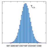
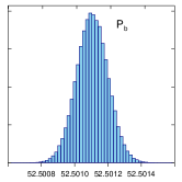
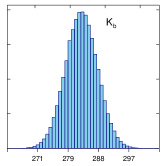
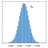
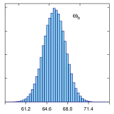
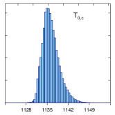
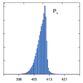
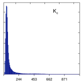
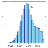
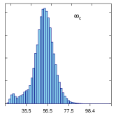
Figure 9.— MCMC marginalized posterior distributions of the radial-velocity orbital parameters for the Kepler-432 system. While the inner planet (top row) has a well-constrained solution, it is clear from the marginalized distributions that there is a tail of high eccentricity outer orbits (bottom row) that cannot be ruled out by the current RV data. This tail can also be seen in the joint mass-eccentricity posterior shown in the stability analysis of Figure 11.

6. Orbital Solution

After recognition of the signature of the non-transiting planet in the Kepler-432 RVs (the outer planet was identified both visually and via periodogram analysis), they were fit with two Keplerian orbits using a MCMC algorithm with the Metropolis-Hastings rule (Metropolis et al., 1953; Hastings, 1970) and a Gibbs sampler (a review of which can be found in Casella & George, 1992). Twelve parameters were included in the fit: for each planet, the times of inferior conjunction $T_{\rm 0}$, orbital periods $P$, radial-velocity semi-amplitudes $K$, and the orthogonal quantities $\sqrt{e}\sin{\omega}$ and $\sqrt{e}\cos{\omega}$, where $e$ is orbital eccentricity and $\omega$ is the longitude of periastron; the systemic velocity, $\gamma_{\rm rel}$, in the arbitrary zero point of the TRES relative RV data set; and the FIES RV offset, ${\Delta}RV_{\rm FIES}$. (The absolute systemic velocity, $\gamma_{\rm abs}$, was calculated based on $\gamma_{\rm rel}$ and the offset between relative and absolute RVs, which are discussed in Section 4.) We applied Gaussian priors on $T_{\rm 0,b}$ and $P_{\rm b}$ based on the results of the light curve fitting.

Table 5Kepler-432 Planetary Properties

Parameter	Without N-Body	With N-Body
Inner Planet
$T_{\rm 0,b}$ (BJD)	$2455949.5374^{+0.0018}_{-0.0016}$	$2455949.5374^{+0.0011}_{-0.0012}$
$P_{\rm b}$ (days)	$52.501134^{+0.000070}_{-0.000107}$	$52.501129^{+0.000067}_{-0.000053}$
$K_{\rm b}$ (m s-1)	$285.9^{+4.1}_{-4.7}$	$286.8^{+4.7}_{-4.0}$
$\sqrt{e_{\rm b}}\cos{\omega_{\rm b}}$	$0.294^{+0.022}_{-0.015}$	$0.311^{+0.018}_{-0.016}$
$\sqrt{e_{\rm b}}\sin{\omega_{\rm b}}$	$0.6482^{+0.0134}_{-0.0094}$	$0.645^{+0.012}_{-0.011}$
$e_{\rm b}$	$0.5121^{+0.0084}_{-0.0107}$	$0.5134^{+0.0098}_{-0.0089}$
$\omega_{\rm b}$ (deg)	$65.6^{+1.5}_{-1.8}$	$64.1^{+1.6}_{-1.5}$
$i_{b}$ (deg)	$88.17^{+0.61}_{-0.33}$	$88.17^{+0.61}_{-0.33}$
$M_{\rm b}$ ($M_{\rm Jup}$)	$5.41^{+0.30}_{-0.19}$	$5.41^{+0.32}_{-0.18}$
$R_{\rm b}$ ($R_{\rm Jup}$)	$1.145^{+0.036}_{-0.039}$	$1.145^{+0.036}_{-0.039}$
$\rho_{\rm b}~{}({\rm g\,cm}^{-3})$	$4.46^{+0.36}_{-0.29}$	$4.46^{+0.37}_{-0.29}$
$a_{\rm b}$ (AU)	$0.301^{+0.016}_{-0.011}$	$0.301^{+0.016}_{-0.011}$
$\langle F_{\rm b}\rangle$ ($\langle F_{\oplus}\rangle$)	$118\pm 10$	$118\pm 10$
Outer Planet
$T_{\rm 0,c}$ (BJD)	$2456134.9^{+3.0}_{-2.1}$	$2456139.3^{+3.6}_{-2.9}$
$P_{\rm c}$ (days)	$411.0^{+0.9}_{-3.2}$	$406.2^{+3.9}_{-2.5}$
$K_{\rm c}$ (m s-1)	$73^{+25}_{-15}$	$62.1^{+6.1}_{-5.8}$
$\sqrt{e_{\rm c}}\cos{\omega_{\rm c}}$	$0.47^{+0.12}_{-0.14}$	$0.336^{+0.115}_{-0.076}$
$\sqrt{e_{\rm c}}\sin{\omega_{\rm c}}$	$0.648^{+0.072}_{-0.073}$	$0.602^{+0.048}_{-0.071}$
$e_{\rm c}$	$0.64^{+0.14}_{-0.13}$	$0.498^{+0.029}_{-0.059}$
$\omega_{\rm c}$ (deg)	$53.2^{+8.7}_{-9.5}$	$60.8^{+7.0}_{-11.2}$
$M_{\rm c}\sin{i_{\rm c}}$ ($M_{\rm Jup}$)	$2.63^{+0.43}_{-0.35}$	$2.43^{+0.22}_{-0.24}$
$a_{\rm c}\sin{i_{\rm c}}$ (AU)	$1.188^{+0.062}_{-0.042}$	$1.178^{+0.063}_{-0.042}$
$\langle F_{\rm c}\rangle$ ($\langle F_{\oplus}\rangle$)	$8.5^{+2.1}_{-1.2}$	$7.7^{+0.7}_{-0.8}$
Other Parameters
$\gamma_{\rm rel}$ (m s-1)	$313.4^{+5.1}_{-4.5}$	$306.7^{+2.6}_{-2.7}$
$\gamma_{\rm abs}$ (km s-1)	$-35.22\pm 0.19$	$-35.22\pm 0.19$
$\Delta RV_{\rm FIES}$ (m s-1)	$-493.5^{+8.4}_{-10.4}$	$-490.5^{+8.6}_{-7.7}$
RV Jitter (m s-1)	$20$	$20$

Note. — The first set of parameters comes from the the photometric, radial-velocity, and asteroseismic analyses, and the second set incorporates additional constraints from the stability analysis of our N-body simulations. We adopt the properties derived with constraints from the N-body simulations.

We ran a chain with $1.01\times 10^{7}$ steps, treating the first $10^{5}$ realizations as burn-in and thinning the chain by saving every tenth entry, for a final chain length of $10^{6}$. The marginalized posterior distributions are shown in Figure 9. It is apparent that while the parameters of the inner planet are very well constrained, there is a high-eccentricity tail of solutions for the outer planet that cannot be ruled out by RVs alone (we investigate this further using N-body simulations in Section 8). Because several of the posteriors are non-Gaussian, we cannot simply adopt the median and central $68.3\%$ confidence interval as our best fit parameters and $1$-$\sigma$ errors as we normally might. Instead, we adopt best fit parameters from the mode of each distribution, which we identify from the peak of the probability density function (PDF). We generate the PDFs using a Gaussian kernel density estimator with bandwidths for each parameter chosen according to Silverman’s rule. We assign errors from the region that encloses $68.3\%$  of the PDF, and for which the bounding values have identical probability densities. That is, we require the $\pm 1$-$\sigma$ values to have equal likelihoods. The resulting orbital solution using these parameters has velocity residuals larger than expected from the nominal RV uncertainties. We attribute this to some combination of astrophysical jitter (e.g., stellar activity or additional undetected planets) and imperfect treatment of the various noise sources described in Section 4. An analysis of the residuals does not reveal any significant periodicity, but given our measurement precision, we would not expect to detect any additional planets unless they were also massive gas giants, or orbiting at very small separations. To account for the observed velocity residuals, we re-run our MCMC with the inclusion of an additional RV jitter term. Tuning this until $\chi^{2}$ is equal to the number of degrees of freedom, we find an additional $20~{}{\rm m\thinspace s^{-1}}$ jitter is required. While part of this jitter may be due to instrumental effects, we do not include separate jitter terms for the TRES and FIES RVs because the FIES data set is not rich enough to reliably determine the observed scatter. We report the best fit orbital and physical planetary parameters in Table 5, which also includes the set of parameters additionally constrained by dynamical stability simulations, as described in the N-body analysis of Section 8. The corresponding orbital solution is shown in Figure 10.

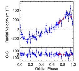
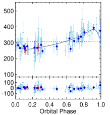
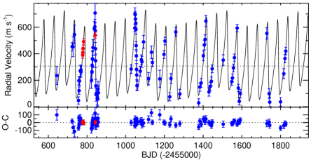
Figure 10.— The individual components of the orbital fit corresponding to planets b (top left) and c (top right), and the combined RV timeseries (bottom). TRES RVs are plotted in blue and FIES RVs are plotted in red. For planet c, we plot the individual RVs in light blue and the binned data in dark blue. Velocity residuals are plotted in the corresponding lower panels. The plotted error bars include both the internal errors and the $20$ m s^-1 jitter that was added to the uncertainties during the fitting process.

7. False Positive Scenarios

An apparent planetary signal (transit or RV) can sometimes be caused by astrophysical false positives. We consider several scenarios in which one of the Kepler-432 planetary signals is caused by something other than a planet, and we run a number of tests to rule these out.

For an object with a deep transit, such as Kepler-432b, one may worry that the orbiting object is actually a small star, or that the signal is caused by a blend with an eclipsing binary system. Sliski & Kipping (2014) noted that there are very few planets orbiting evolved stars with periods shorter than $100$ days (Kepler-432b would be somewhat of an outlier), and also found via AP that either the transit signal must be caused by a blend, or it must have significant eccentricity ($e>0.488$). Without additional evidence, this would be cause for concern, but our radial velocity curve demonstrates that the transiting object is indeed orbiting the target star, that its mass is planetary, and, consistent with the prediction of Sliski & Kipping (2014), its eccentricity is $0.5134$.

If a planet does not transit, as is the case for Kepler-432c, determining the authenticity of the planetary signal is less straightforward. An apparent radial-velocity orbit can be induced by a genuine planet, spots rotating on the stellar surface (Queloz et al., 2001), or a blended stellar binary (Mandushev et al., 2005). Both of these false positive scenarios should manifest themselves in the shapes of the stellar spectral lines. That is, spots with enough contrast with the photosphere to induce apparent RV variations will also deform the line profiles, as should blended binaries bright enough to influence the derived RVs. A standard prescription for characterizing the shape of a line is to measure the relative velocity at its top and bottom; this difference is referred to as a line bisector span (see, e.g., Torres et al., 2005). To test against the scenarios described, we computed the line bisector spans for the TRES spectra. We do find a possible correlation with the RVs of the outer planet, having a Spearman’s rank correlation value of $-0.21$ and a significance of $94\%$. While this is a potential concern and we cannot conclusively demonstrate the planetary nature of the $407$-day signal, we find it to be the most likely interpretation. In the following paragraphs, we explain why other interpretations are unlikely.

With the discovery of a close stellar companion (see Section 3.2), it is reasonable to ask how that might affect interpretation of the outer planetary signal. That is, if the stellar companion is itself a binary with a period of $\mathord{\sim}400$ days, could it cause the RV signal we observe? The answer is unequivocally no, as the companion is far too faint in the optical compared to the primary star ($\Delta V\mathord{\sim}7$) to contribute any significant light to the spectrum, let alone induce a variation of $\mathord{\sim}100~{}{\rm m\thinspace s^{-1}}$ or affect the bisector spans. If there is also a brighter visual companion inside the resolution limit of our high resolution images ($\mathord{\sim}0\farcs 05\simeq 45$ AU projected separation), it could be a binary with a $400$-day period responsible for the RV and bisector span variations on that timescale. However, such a close physically bound binary may pose problems for formation of the $52.5$-day planet, and the a priori likelihood of a background star bright enough to cause the observed variations within $0.05\arcsec$  is extremely low; a TRILEGAL simulation suggests $\mathord{\sim}5\times 10^{-6}$ background sources should be expected, and only a small fraction of those would be expected to host a binary with the correct systemic velocity.

To rule out spot-induced velocity variation, we examine the Kepler light curve for evidence of spot activity. From the measured $v\sin{i_{\star}}$, $i_{\star}$, and $R_{\star}$, the stellar rotation period is $77\pm 14$ days. Not only is this inconsistent with the observed outer orbital period ($407$ days), but we detect no significant photometric signal near either of these periods. For Kepler-432 ($v\sin{i_{\star}}=2.7~{}{\rm km\thinspace s^{-1}}$), a spot must cover $\mathord{\sim}4$%–$5$% of the stellar surface to induce the observed RV amplitude (Saar & Donahue, 1997), and such a spot would have been apparent in the high precision Kepler light curve.

As we have shown in Section 5, Kepler-432 exhibits strong oscillations, so one may wonder whether these could induce the observed RV signal for the outer planet. Oscillations on a $400$-day timescale are intrinsically unlikely, as there is no known driving mechanism that could cause them in giant stars; the well-known stochastically driven oscillations are confined to much higher frequencies. Furthermore, if there were such a mechanism, a mode with $\mathord{\sim}50~{}{\rm m\thinspace s^{-1}}$ velocity semi-amplitude should cause a photometric variation of $\mathord{\sim}1.3$ mmag (see Kjeldsen & Bedding, 1995), which is clearly ruled out by the Kepler data.

Upon examining all of the evidence available, we conclude that both detected orbits are caused by bona fide planets orbiting the primary star.

8. Orbital Stability Analysis

8.1. Methodology

Following the Keplerian MCMC fitting procedure described in Section 6, we wish to understand whether these posterior solutions are dynamically stable—i.e., whether they describe realistic systems which could survive to the $3.5$ Gyr age of the system. When presenting our results in the sections that follow, we use the planet–planet separation as an easily visualized proxy for stability: given the semi-major axes of the two planets—$\mathord{\sim}0.3$ and $\mathord{\sim}1.2$ AU—separations greater than $\mathord{\sim}10$ AU are clear indications that the system has suffered an instability and the planets subsequently scattered. If some solutions do prove to be unstable, it will lead to further constraints on the orbital elements, and thus the planetary masses. We perform integrations of both coplanar and inclined systems. We first explore the less computationally expensive coplanar case to understand the behavior of the system, and then extend the simulations to include inclination in the outer orbit, which has the additional potential to constrain the mutual inclination of the planets.

To understand this stability, we utilize the integration algorithm described in Payne et al. (2013). This algorithm uses a symplectic method in Jacobi coordinates, making it both accurate and rapid for systems with arbitrary planet-to-star mass ratios. It uses calculations of the tangent equations to evaluate the Lyapunov exponents for the system, providing a detailed insight into whether the system is stable (up to the length of the simulation examined) or exhibits chaos (and hence instability).

For the coplanar systems, we take the ensemble of $10^{6}$ solutions generated in Section 6 (which form the basis of the reported elements in column 2 of Table 5) and convert these to Cartesian coordinates, assuming that the system is coplanar and edge-on ($90^{\circ}$), and hence both planets have their minimum masses. We then evolve the systems forward for a fixed period of time (more detail supplied in Section 8.2 below) and examine some critical diagnostics for the system (e.g., the Lyapunov time, and the planet–planet separation) to understand whether the system remains stable, or whether some significant instability has become apparent.

For the inclined systems, we assume that the inner (transiting) planet is edge-on, and hence retains its measured mass. However, the outer planet is assigned an inclination that is drawn randomly from a uniform distribution $0^{\circ}<i_{\rm c}<90^{\circ}$, and its mass is scaled by a factor $1/\sin{i_{\rm c}}$. As such, the outer planet can have a mass that is significantly above the minimum values used in the coplanar case. The longitude of ascending node for the outer planet is drawn randomly from a uniform distribution between $0$ and $2\pi$. We then proceed as in the coplanar case, integrating the systems forward in time to understand whether the initial conditions chosen can give rise to long-term stable systems.

Rauch & Holman (1999) demonstrated that $\sim 20$ timesteps per inner-most orbit is sufficient to ensure numerical stability in symplectic integrations. As the inner planet has a period $\mathord{\sim}50$ days, we use a timestep of $1$ day in all of our simulations, ensuring that our integrations will comfortably maintain the desired energy conservation and hence numerical accuracy.

8.2. Coplanar Stability

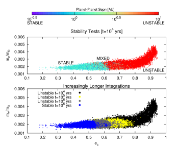
Figure 11.— Top: in the mass-eccentricity plane for the outer planet ($m_{c},e_{c}$), we plot the separation between the two planets in the system at $t=10^{4}$ yr using the color scheme at the top of the plot. A separation greater than $\sim 10$ AU is an indication that the system has suffered an instability and the planets subsequently scattered. Systems with eccentricity $e_{c}\mathrel{\hbox to0.0pt{\lower 4.0pt\hbox{\hskip 1.0pt$\sim$}\hss}\raise 1.0pt\hbox{$>$}}0.75$ are clearly unstable, while those with $e_{c}\mathrel{\hbox to0.0pt{\lower 4.0pt\hbox{\hskip 1.0pt$\sim$}\hss}\raise 1.0pt\hbox{$<$}}0.55$ are clearly stable for $t=10^{4}$ yr. Bottom: in the $(m_{c},e_{c})$ plane, we plot the systems which are unstable at $10^{4}$ yr in black, $10^{5}$ yr in yellow and $10^{6}$ yr in gray, and those that remain stable at $10^{6}$ yr in blue. The systems which are long-term stable in these coplanar simulations occupy a region of parameter space confined to eccentricities $e_{c}\mathrel{\hbox to0.0pt{\lower 4.0pt\hbox{\hskip 1.0pt$\sim$}\hss}\raise 1.0pt\hbox{$<$}}0.55$.

We begin by taking a random selection of $10^{5}$ of the $10^{6}$ solutions from Section 6 and integrating them for a period of $10^{4}$ yr ($3\times 10^{6}$ timesteps). While this is not a particularly long integration period compared with the period of the planets ($\mathord{\sim}50$ and $\mathord{\sim}400$ days), we demonstrate that even during this relatively short integration, approximately half of the systems become unstable. Tellingly, the unstable systems all tend to be the systems in which the outer planet has particularly high eccentricity. We illustrate this in Figure 11, where we plot the mass-eccentricity plane for the outer planet ($m_{\rm c},e_{\rm c}$) and plot the separation between the two planets in the system at $t=10^{4}$ yr. As described above, separations greater than $\mathord{\sim}10$ AU indicate that the system has suffered an instability. This initial simulation clearly demonstrates that at $t=10^{4}$ yr essentially all systems with $e_{\rm c}>0.8$ are unstable, all those with $e_{\rm c}<0.45$ are stable, and those with $0.45<e_{\rm c}<0.8$ are “mixed,” with some being stable and some being unstable.

Given this promising demonstration that the dynamical integrations can restrict the set of solutions, we go on to integrate the systems for increasingly longer periods of time. To save on integration time/cost, we only select the stable solutions from the previous step, and then extend the integration time by an order of magnitude, perform a stability analysis, and repeat. By this method, the $10^{5}$ systems at $t=0$ are reduced to $\mathord{\sim}4.4\times 10^{4}$ stable systems at $10^{4}$ yr, $\mathord{\sim}2.5\times 10^{4}$ stable systems at $10^{5}$ yr, and $\mathord{\sim}9.4\times 10^{3}$ stable systems at $10^{6}$ yr. We illustrate in Figure 11 the successive restriction of the parameter space in the mass-eccentricity plane for the outer planet ($m_{\rm c},e_{\rm c}$) as the integration timescales increase. We find that the long-term stable systems occupy a significantly smaller region of parameter space in the $m_{\rm c},e_{\rm c}$ plane. In particular, we see the eccentricity of the outer planet is restricted to $e_{\rm c}\mathrel{\hbox to0.0pt{\lower 4.0pt\hbox{\hskip 1.0pt$\sim$}\hss}\raise 1.0pt\hbox{$<$}}0.55$.

Using the $\mathord{\sim}9.4\times 10^{3}$ systems which remained stable at $10^{6}$ yr, we use the same method as in Section 6 to determine a new set of best-fit orbital paramters. That is, we use a Gaussian kernel density estimator to smooth the posterior distribution and select the mode (i.e., the value with the largest probability density). The errors correspond to values with equal probability density that enclose the mode and $68.3\%$ of the PDF. The most significant changes in the best-fit parameters occurred for the outer planet, most notably for eccentricity and velocity semi-amplitude, resulting in smaller and more symmetric error bars and a revision in the best-fit minimum mass for planet c.

8.3. Inclined-system Stability

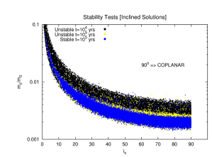
Figure 12.— Stability of systems in the mass-orbital inclination plane of the outer planet ($m_{\rm c},i_{\rm c}$), with black points going unstable within $10^{4}$ yr and yellow points within $10^{5}$ yr, and blue points representing stable systems after integrating for $10^{5}$ yr. The results mirror those of the coplanar case—at all inclinations, the low-mass (low-eccentricity) systems remain stable, while the high-mass (high-eccentricity) systems do not survive long integrations. As some systems remain stable even for highly inclined orbits ($i_{\rm c}\mathord{\sim}0^{\circ}$), we are unable to put strong constraints on the mutual inclination of the planets.

In a manner similar to the coplanar analysis of Section 8.2, we begin by taking all $10^{6}$ solutions from Section 6 and integrating them for a period of $10^{4}$ yr ($3\times 10^{6}$ timesteps). However, in these inclined system integrations, the outer planet has an inclination that is not edge-on, and hence a mass for the outer planet that is inflated compared to its minimum edge-on value, as described in Section 8.1.

A much larger fraction of the inclined systems become unstable in the first $10^{4}$ yr, and we find that the $N=10^{6}$ systems at $t=0$ are reduced to $N\mathord{\sim}1.5\times 10^{5}$ stable systems at $10^{4}$ yr. Integrating these stable systems while keeping the pre-assigned inclinations for the outer planet (i.e., we do not re-randomize the inclinations) we integrate this subset on to $10^{5}$ yr, and find that the number of stable systems subsequently reduces to $N\mathord{\sim}10^{4}$. We plot these stability results as a function of mass and inclination of the outer planet in Figure 12.

We find that the vast majority of the stable solutions are (somewhat unsuprisingly) restricted to the range of parameter space with relative inclinations $\mathrel{\hbox to0.0pt{\lower 4.0pt\hbox{\hskip 1.0pt$\sim$}\hss}\raise 1.0pt\hbox{$<$}}70^{\circ}$ (i.e., $i_{\rm c}\mathrel{\hbox to0.0pt{\lower 4.0pt\hbox{\hskip 1.0pt$\sim$}\hss}\raise 1.0pt\hbox{$>$}}20^{\circ}$ in Figure 12). There is a small population with significantly higher eccentricities and relative inclinations that remains stable at $t=10^{5}$ yr, and it is possible that these systems exhibit strong Kozai oscillations, but their long-term ($>10^{5}$ yr) behavior has not been investigated. We emphasize that the inclinations and longitudes of the ascending node were assigned randomly, and hence it is possible that specifically chosen orbital alignments could allow for enhanced stability in certain cases. Unfortunately, because some systems remain stable even for highly inclined outer orbits ($i_{c}\mathord{\sim}0^{\circ}$), we are unable to strongly constrain the mutual inclination of the planetary orbits.

We also note that the presence of a distant stellar companion (as detected in our AO images) or additional, as yet undetected, planets (as may be suggested by the excess RV scatter) could influence the long-term stability of the systems simulated herein. The evolution of the star on the red giant branch is also likely to affect the orbital evolution (especially for the inner planet; see Section 9), but it is not important over the $10^{6}$-year timescales of these simulations. Simulating the effect of poorly characterized or hypothetical orbits, or the interactions between expanding stars and their planets, is beyond the scope of the current paper, and instead we simply remind the reader of these complications. We present planetary properties derived with and without constraints from our simulations (Table 5) so that the cautious reader may choose to adopt the more conservative (and poorly determined) parameters of the outer orbit in any subsequent analysis.

9. Discussion

The properties of the star and planets of Kepler-432 are unusual in several ways among the known exoplanets, which makes it a valuable system to study in detail. For example, it is a planetary system around an intermediate mass star (and an evolved star), it hosts a planet of intermediate period, and it hosts at least one very massive transiting planet. Close examination of the system may provide insight into the processes of planet formation and orbital evolution in such regimes. Kepler-432 is also the first planet orbiting a giant star to have its eccentricity independently determined by RVs and photometry, which helps address a concern that granulation noise in giants can inhibit such photometric measurements.

9.1. Comparing the Eccentricity from AP versus RVs

AP provides an independent technique for measuring orbital eccentricities with photometry alone, via the so-called photoeccentric effect (Dawson & Johnson, 2012), and can be used as a tool to evaluate the quality of planet candidates (Tingley et al., 2011). It was originally envisioned as a technique for measuring eccentricities (Kipping et al., 2012), but other effects, such as a background blend, can also produce AP effects (Kipping, 2014a). Given that we here have an independent radial velocity orbital solution, there is an opportunity to compare the two independent solutions, allowing us to comment on the utility of AP.

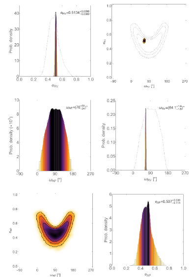
Figure 13.— The marginalized and joint posterior distributions of $e$ and $\omega$, as determined by AP and RVs. The three panels in the lower left are from AP; the three in the upper right (the narrow histograms and well-constrained joint distribution) are from RVs, which also show the AP distributions overplotted as thin gray dotted lines for comparison.

Kepler-432b was previously analyzed as part of an ensemble AP analysis by Sliski & Kipping (2014). In that work, the authors concluded that Kepler-432b displayed a strong AP effect, either because the candidate was a false-positive or because it exhibited a strong photoeccentric effect with $e\geq 0.488_{-0.051}^{+0.025}$. Our analysis, using slightly more data and a full $\omega$ marginalization is excellent agreement with that result, finding $e=0.507^{+0.039}_{-0.114}$ and $\omega=76^{+59}_{-24}$ deg. The AP results may be compared to that from our radial velocity solution, where again we find excellent agreement, since RVs yield $e=0.5134^{+0.0098}_{-0.0089}$ and $\omega=64.1^{+1.6}_{-1.5}$ deg. The results may be visually compared in Figure 13. We note that this is not the first time AP and RVs have been shown to yield self-consistent results, with Dawson & Johnson (2012) demonstrating the same for the Sun-like star HD 17156b. However, this is the first time that this agreement has been established for a giant host star. This is particularly salient in light of the work of Sliski & Kipping (2014), who find that the AP deviations of giant stars are consistently excessively large. The authors proposed that many of the KOIs around giant stars were actually orbiting a different star, with the remaining being eccentric planets around giant stars. Kepler-432b falls into the latter category, consistent with its original ambiguous categorization as being either a false positive or photoeccentric.

The analysis presented here demonstrates that AP can produce accurate results for giant stars. This indicates that the unusually high AP deviations of giant stars observed by Sliski & Kipping (2014) cannot be solely due to time-correlated noise caused by stellar granulation, which has recently been proposed by Barclay et al. (2015) to explain the discrepancy between AP and radial velocity data for Kepler-91b. However, time-correlated noise may still be an important factor in giant host stars which are more evolved than Kepler-432 (such as Kepler-91), for which granulation becomes more pronounced (Mathur et al., 2011). To further investigate these hypotheses, we advocate for further observations of giant planet-candidate host stars to resolve the source of the AP anomalies.

9.2. A Benchmark for Compositions of Super-Jupiters

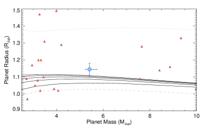
Figure 14.— The masses and radii of known giant planets (red triangles) and Kepler-432b (blue circle). Overplotted as solid black lines are a series of planetary models (Fortney et al., 2007) with age $3.5$ Gyr, an appropriate semi-major axis, and core masses $0$, $10$, $25$, $50$, and $100~{}{M_{\oplus}}$ (from top to bottom). Also plotted are models for young ($100$ Myr), hot ($0.02$ AU), coreless planets (dotted gray line); and old ($10$ Gyr), cool ($1$ AU) planets with massive ($100~{}{M_{\oplus}}$) cores (dashed gray line). These roughly illustrate the range of sizes possible for a given mass.

Kepler-432b has a measured mass, radius, and age, which allows us to investigate its bulk composition. Among transiting planets—i.e., those for which interior modeling is possible—there are only $11$ more massive than $4.5~{}{M_{\rm Jup}}$. We also point out the gap in the center of the plot in Figure 14; no planets with masses between $4$ and $7.25~{}{M_{\rm Jup}}$ also have measured radii, so Kepler-432b immediately becomes a valuable data point to modelers. Moreover, most of the super-Jupiters are highly irradiated, which further complicates modeling and interpretation of planetary structure. Kepler-432b receives only about $20\%$ of the insolation of a $3$-day hot Jupiter orbiting a Sun-like star. Because of this, it may prove to be an important benchmark for planetary interior models—for example, as a means of checking the accuracy of models of super-Jupiters without the complication of high levels of incident flux. In Figure 14, we compare the mass and radius of Kepler-432b to age- and insolation-appropriate planetary models (Fortney et al., 2007) of varying core mass. We interpolate the models to a planet with the age of Kepler-432 ($3.5$ Gyr) in a circular orbit of $0.092$ AU around a Sun-like star (the insolation of which is identical to the time-averaged insolation of Kepler-432b on its more distant eccentric orbit around a more luminous star). The radius is apparently slightly inflated, but is somewhat consistent ($1$-$\sigma$) with that of a planet lacking a core of heavy elements. This is not an iron-clad result, though; the radius even agrees with the prediction for a planet with a $50~{}{M_{\oplus}}$ core to within $1.5$-$\sigma$. Nevertheless, we interpret this as evidence that Kepler-432b most likely has only a small core of heavy elements.

9.3. Jupiters Do (Briefly) Orbit Giants Within $0.5$ AU

As discussed previously, we do not know of many transiting giant planets orbiting giant stars. This is not because giant planets orbiting the progenitors to giant stars are rare; due in part to survey strategies, giant stars are, on average, more massive than the known main-sequence planet hosts, and massive stars seem to be more likely to harbor massive planets. However, because very few giant stars host planets inside $1$ AU, the a priori probability of a transit is low for these systems. In fact, there are only two other giant planets with a measured mass ($M_{p}>0.5~{}{M_{\rm Jup}}$) transiting a giant star ($\log{g_{\star}}<3.9$)—Kepler-56c (Huber et al., 2013b), and the soon-to-be-swallowed hot Jupiter Kepler-91b (Barclay et al., 2015; Lillo-Box et al., 2014a, b). This makes Kepler-432b important in at least two respects: it is a rare fully characterized giant planet transiting a giant star, and it is a short-period outlier among giant planets orbiting giant stars (see Figure 15). Kepler-432b thus gives us a new lens through which to examine the dearth of short and intermediate period Jupiters ($<0.5$ AU) around giant stars. Kepler-432c, on the other hand, appears to be very typical of Jupiters around evolved stars, in both mass and orbital separation.

After noticing that Kepler-432b sits all alone in the $M_{\rm p}$ versus $a$ parameter space, it is natural to wonder why, and we suggest two potential explanations, each of which may contribute to this apparent planetary desert. In the first, we consider that Kepler-432b may simply be a member of the tail of the period distribution of planets around massive and intermediate-mass main-sequence stars. That is, perhaps massive main-sequence stars simply harbor very few planets with separations less than $1$ AU. If this occurrence rate is a smooth function of stellar mass, then because Kepler-432 would most accurately be called intermediate mass, it might not be so surprising that it harbors a planet with a separation of $0.3$ AU while its more massive counterparts do not. If this is the case, then as we detect more giant planets orbiting giant stars (and main-sequence stars above the Kraft break), we can expect to find a sparsely populated tail of planets interior to $1$ AU. This may ultimately prove to be responsible for the observed distribution, and would have important implications for giant planet formation and migration around intermediate mass stars in comparison to Sun-like stars, but it cannot be confirmed now. It will require additional planet searches around evolved stars and improvements in detecting long period planets orbiting rapidly rotating main-sequence stars.

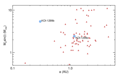
Figure 15.— All planets with minimum masses $M_{\rm p}\sin{i}>0.5~{}{M_{\rm Jup}}$ orbiting giant stars ($\log{g_{\star}}<3.9$), plotted as red triangles. Kepler-432b and c are labeled and plotted as large blue circles.

In the second scenario, we consider that Kepler-432b may be a member of a more numerous group of planets interior to $\mathord{\sim}0.5$ AU that exist around main-sequence F- and A-type stars, but do not survive through the red giant phase when the star expands to a significant fraction of an AU. If this is the case, then Kepler-432b is fated to be swallowed by its star through some combination of expansion of the stellar atmosphere and orbital decay, and we only observe it now because Kepler-432 has only recently begun its ascent up the red giant branch. Suggestively, the resulting system that would include only Kepler-432c would look much more typical of giant stars. In this scenario, planets must begin their orbital decay very soon after the star evolves off of the main sequence, or we would expect to observe many more of them. Assuming, then, that Kepler-432b is close enough to its host to have started its orbital decay, we may be able to detect evidence of tidal or magnetic SPI (see, e.g., Shkolnik et al., 2009). As the star expands those interactions would strengthen, which should lead to more rapid orbital decay. While typically tidal interaction leading to circularization and orbital decay has been modeled to depend only on tides in the planet, Jackson et al. (2008) show that tides in the star (which are strongly dependent on the stellar radius) can also influence orbital evolution. This provides a tidal mechanism for more distant planets to experience enhanced orbital evolution as the star expands. Recent simulations by Strugarek et al. (2014) further demonstrate that in some scenarios (especially with strong stellar magnetic fields and slow rotation), magnetic SPI can be as important to orbital migration as tidal SPI, and can lead to rapid orbital decay. Kepler-432 does rotate slowly, and the results of a two-decade survey by Konstantinova-Antova et al. (2013) reveal that giants can exhibit field strengths up to $\mathord{\sim}100$ G. Encouraged by these findings, we search for evidence of SPI in the Kepler-432 system in Section 9.5.

The hypothetical scenario in which planets inside $\mathord{\sim}0.5$ AU around massive and intermediate-mass stars ultimately get destroyed may also help explain the properties of the observed distribution of planets orbiting evolved stars. If planets form on circular orbits, then in order to excite large eccentricities, a planet must experience dynamical interaction with another planet (e.g., Rasio & Ford, 1996; Juric & Tremaine, 2008) or another star (e.g., Fabrycky & Tremaine, 2007; Naoz et al., 2012). More massive stars (like many of those that have become giants) are more likely than lower mass, Sun-like stars to form giant planets, and they are also more likely to have binary companions (e.g., de Rosa et al., 2014; Raghavan et al., 2010), so one might expect the typical planet orbiting a giant star to be more eccentric, not less. However, the most eccentric planets around evolved stars would have pericenter distances near, or inside the critical separation at which planets get destroyed. This could lead either to destruction by the same mechanisms as the close-in planets, or to partial orbital decay and circularization. The consequence of either process would be more circular orbits on average and an overabundance of planets at separations near the critical separation ($0.5\,{\rm AU}\mathrel{\hbox to0.0pt{\lower 4.0pt\hbox{\hskip 1.0pt$\sim$}\hss}\raise 1.0pt\hbox{$<$}}a\mathrel{\hbox to0.0pt{\lower 4.0pt\hbox{\hskip 1.0pt$\sim$}\hss}\raise 1.0pt\hbox{$<$}}1\,{\rm AU}$), which is indeed observed. For similar arguments and additional discussion, see Jones et al. (2014). Counterarguments articulated by those authors include that massive subgiants do not seem to host many planets inside $1$ AU either, but subgiants are not large enough to have swallowed them yet. This might point toward a primordial difference in the planetary period distribution between Sun-like and more massive stars, rather than a difference that evolves over time.

9.4. Implications for Giant Planet Formation and Migration

Assuming that giant planets form beyond the ice line (located at $\mathord{\sim}4.9$ AU for a star with $M\mathord{\sim}1.4~{}{M_{\odot}}$, using the approximation of Ida & Lin, 2005), both Kepler-432b and c have experienced significant inward migration. At first glance, their large orbital eccentricities would suggest that they have experienced gravitational interactions, perhaps during one or more planet–planet scattering events that brought them to their current orbital distances, or through the influence of an outer companion (like that detected in our AO images). However, the apparent alignment between the stellar spin axis and the orbit of the inner planet presents a puzzle; if the (initially circular, coplanar) planets migrated via multi-body interactions, we would expect both the eccentricities and the inclinations to grow. It is possible, of course, that by chance the inner planet remained relatively well-aligned after scattering, or that the planets experienced coplanar, high-eccentricity migration, which has recently been suggested as a mechanism for producing hot Jupiters (Petrovich, 2014). Measuring the mutual inclination between the planets could lend credence to one of these scenarios. Unfortunately, because we are unable to constrain the mutual inclination of the planets, we cannot say whether they are mutually well-aligned (which would argue against planet-planet scattering) or not.

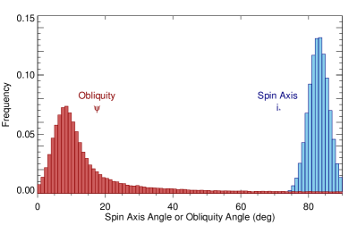
Figure 16.— An underlying distribution of true obliquities, $\psi$, corresponding to a hypothetical measured stellar inclination, $i_{\star}$. A system with edge-on rotation has $i_{\star}=90^{\circ}$, and $\psi=0^{\circ}$ indicates perfect alignment between stellar spin and planetary orbital angular momentum. The long tail of high obliquities illustrates that even with a nearly edge-on stellar spin, a transiting planet may still be misaligned.

At this point, it is prudent to reiterate that the stellar spin and orbital angular momenta are measured to be nearly aligned only as projected along the line of sight. The true obliquity is unknown, and may be significantly non-zero. In Figure 16, we illustrate this by simulating the underlying obliquity distribution that corresponds to an example $i_{\star}$ distribution with a mean of $83^{\circ}$, similar to that measured from asteroseismology. To generate this obliquity distribution, we draw from $i_{\star}$ and a random uniform azimuthal angle, $\theta$, and calculate the true obliquity, $\psi$. As is apparent from the $\psi$ distribution, while it is likely that the true obliquity is low, there is a tail of highly misaligned systems (representing those with spin axes lying nearly in the plane of the sky but not coincident with the orbital angular momentum) that could produce the stellar inclination we observe. Ideally, we would also measure the sky-projected spin–orbit angle, $\lambda$, in order to detect any such conspiring misalignment and calculate the true obliquity. However, there is not an obvious way to do this: the slow rotation, long period, and lack of star spots render current techniques to measure the sky-projected obliquity ineffective. We are left with an inner planet that is likely, but not certainly, aligned with the stellar spin axis, and an unknown inclination of the outer orbital plane.

The likely alignment of the inner planet seems at odds with the large orbital eccentricities and the assumption that multi-body interactions are responsible for their migration, but we have thus far neglected interaction between the planets and the host star. In their investigation of hot Jupiter obliquities, Winn et al. (2010) suggested that well-aligned hot Jupiters may have been misaligned previously, and that subsequent tidal interaction may have realigned the stellar rotation with the planetary orbit, perhaps influencing the convective envelope independently of the interior. This idea was furthered by Albrecht et al. (2012), who found that systems with short tidal-dissipation timescales are likely to be aligned, while those with long timescales are found with a wide range of obliquities. In the following section, we explore the possibility that Kepler-432b has undergone a similar evolution, obtaining an inclined orbit through its inward migration, but subsequently realigning the stellar spin.

9.5. Evidence for Spin–Orbit Evolution

During the main-sequence lifetime of Kepler-432, the current position of the planets would be too far from the star to raise any significant tides, but the star is now several times its original size, such that at periastron, the inner planet passes within $7.7$ stellar radii of the star. The unusually large planetary mass also helps strengthen tidal interactions. Following Albrecht et al. (2012) (who in turn used the formulae of Zahn, 1977), for Kepler-432 we calculate the tidal timescale for a star with a convective envelope:

$$\tau_{\rm CE}=(10^{10}~{}{\rm yr})q^{-2}\left(\frac{a/R_{\star}}{40}\right)^{6}.$$ (1)

For a radiative atmosphere, as Kepler-432 would have had on the main sequence, the appropriate timescale would be

$$\tau_{\rm RA}=(1.25\times 10^{9}~{}{\rm yr})q^{-2}(1+q)^{-5/6}\left(\frac{a/R_{\star}}{6}\right)^{17/2}.$$ (2)

We repeat the words of caution from Albrecht et al. (2012): these equations are calibrated to star–star interactions rather than star–planet interactions, and are timescales for spin–orbit synchronization, not realignment. As such, the timescales are assumed to be valid only as a relative metric. The authors arbitrarily divided the resulting values by $5\times 10^{9}$ to express this point, and to set the values on a convenient scale. In Figure 17, we have reproduced a version of Figure 24 of Albrecht et al. (2012), showing the relative tidal dissipation timescales for all hot Jupiters with measured spin–orbit angles. We have excluded the same systems they did, and added $9$ recent projected obliquity measurements, including that of Kepler-432b. Their result still holds true; systems with short tidal dissipation timescales are well aligned, while those with long tidal timescales display a wide range of obliquities. We also note that recent work by Valsecchi & Rasio (2014), which includes a more detailed treatment of the convection and stellar evolution of each star, similarly concludes that the observed obliquity distribution can be explained by tidal evolution. While the angle measured for Kepler-432b is the line of sight projection rather than the sky-plane projection, and the efficiency of realignment may be different for evolved stars given their different internal structure, Kepler-432b does have a short tidal timescale, and it sits in a region with hot Jupiter systems that are mostly well-aligned. We interpret this result as evidence that the spin axis of Kepler-432 has been realigned to the orbit of the inner planet by the same mechanism responsible for hot Jupiter realignment.

Alternative mechanisms have been proposed to explain the alignment for hot Jupiters orbiting cool stars. One such alternative, suggested by Dawson (2014), is that the orbital alignment trend with stellar temperature is due to strong versus weak magnetic breaking (for stars below and above the Kraft break), rather than tidal dissipation efficiency as in Albrecht et al. (2012). This has the attractive quality of being part of a theory that is also able to predict the observed mass cut-off for retrograde planets and the trend between planet mass and host star rotation periods. In the Dawson (2014) framework, one may still conclude that Kepler-432 would realign during its red giant phase, but this depends in part on the unknown magnetic properties of the star: the Konstantinova-Antova et al. (2013) finding of strong magnetic fields in some giants may indeed indicate that Kepler-432 possesses a short enough magnetic braking timescale to allow for realignment in this framework, too.

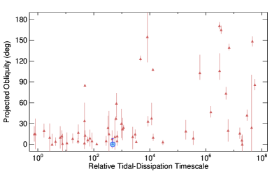
Figure 17.— An adapted version of Figure 24 from Albrecht et al. (2012). We plot the projected obliquity of giant planets versus the relative tidal timescale. We include planets from Albrecht et al. (2012) as well as $8$ more recent spin–orbit measurements from the literature (red triangles) and Kepler-432b (large blue circle). Because it sits in a region with well-aligned hot Jupiters, we posit that Kepler-432b has also realigned the spin of its host star.

In the event that the envelope and the core have different spin axis inclinations, this might manifest itself in the asteroseismic modes. Because $g$-mode-dominated $\ell=1$ modes are most sensitive to core rotation while $p$-mode-dominated mixed modes are most sensitive to the surface, one might obtain different inclination measurements from the different modes. However, our analysis of individual $\ell=1$ modes in Section 5.3 showed they were consistent with $\mathord{\sim}90^{\circ}$ inclination for both core and envelope. This would argue against a realigned envelope for Kepler-432, but a modest misalignment might be undetectable given the degraded precision when fitting modes independently. Furthermore, as shown for the obliquity and spin axis in Figure 16, even if the two spin axes both lie in the sky plane, there is a chance they could be significantly misaligned. Regardless of its efficacy in the case of Kepler-432, asteroseismology may be able to detect a significant misalignment between core and envelope in other systems hosting giant planets with short tidal timescales. If detected, this would be important evidence in the interpretation of giant planet migration, and we suggest this be explored for other systems.

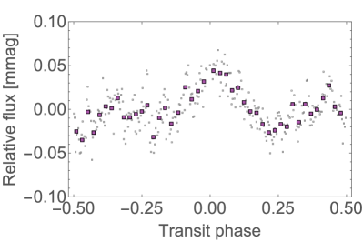
Figure 18.— The Kepler light curve, binned and folded to the period of the transiting planet, with the transits removed. Given that periastron occurs just before transit and the stellar rotation period is longer than the orbital period, the brightening just after transit (orbital phase 0) is what would be expected for a bright spot that is tidally excited during the periastron passage of the planet.

While the evidence presented thus far for realignment of the Kepler-432 system is circumstantial, there may be additional evidence to support the scenario. If tidal forces are strong enough to realign the spin axis of the host star, they may also excite activity on the stellar surface. SPI need not be limited to tidal interaction, though. At closest approach, the planet is only $7.7$ stellar radii from the star, and thus magnetic interaction may also be possible, since the planet passes inside the Alfvén radius ($\mathord{\sim}10\,R_{\star}$). We return to the light curve to look for signs of these interactions. When folded on the orbital period, an interesting feature emerges (see Figure 18). Just after transit, we detect a brightening of $\mathord{\sim}0.05$ mmag that maintains a coherent shape and phase throughout the mission. The simplest explanation for a light curve feature with the period of the planet is a phenomenon associated with the planet. We suggest that SPI excites a bright spot on the stellar photosphere each orbit during periastron passage. Periastron occurs $1.24$ days before transit, and because the rotation period is longer than the orbital period, the spot should rotate onto the meridian and reach maximum apparent brightness slightly after transit, as is observed.

One might argue that if the planet has realigned the stellar spin, it may have also synchronized it to the orbital period—this would cause any long-lived bright spot to create a peak in the light curve when folded to the orbital period. However, to obtain the observed phasing, the spot would have to conveniently occur at the longitude that coincides with the close approach of the planet. There is also no reason to expect a long-lived bright spot on the star, irrespective of its phasing. Furthermore, there exists evidence that the spin is not synchronized to the orbital period anyway. We have measured $R_{\star}$, $i_{\star}$, and $v\sin{i_{\star}}$, so we can estimate the rotation period to be $P_{\rm rot}\mathord{\sim}77\pm 14$ days, which is inconsistent with the orbital period ($P_{\rm orb}=52.5$ days). Thus, a long-lived rotating star spot should not produce a coherent photometric signal when folded to the orbital period. (Similarly, we must conclude that if $P_{\rm rot}\neq P_{\rm orb}$, any planet-induced spot must decay in brightness relatively quickly, or the brightening feature would appear at different phases in each orbit, washing out the coherent signal that we observe.) We do caution that our $v\sin{i_{\star}}$ measurement for this slowly rotating giant could be biased, for example, due to the unknown macroturbulent velocity of Kepler-432. However, even if our measurement of the rotational velocity is incorrect and the rotation period is synchronized to the orbit, we believe a bright star spot phased with the periastron passage of the planet would more easily be attributed to SPI than coincidence.

One additional worry would be that granulation could produce correlated noise that happens to fold coherently on the orbital period. We find this to be an unlikely scenario given the periodogram of the Kepler data (see Figure 19). If granulation produced light curve amplitudes similar to that observed, we would expect several periods to show similar power simply by chance. Instead, we observe the peak power at the second harmonic of the orbital period ($\mathord{\sim}26.2$ days), and very little power at other periods. It is not particularly surprising that the second harmonic, rather than the first, is the strongest peak, especially given that there is some additional structure in the light curve at phases other than around transit.

The observant reader might notice a possible brightening of lower amplitude at phase $\mathord{\sim}0.4$ of the folded light curve. We are not confident that this is real, but if it is, it holds a wealth of information. As mentioned above, any excited spot must decay in brightness quickly, or much of the star would soon be covered in such spots, obfuscating the coherent signal that we observe. If, however, a spot excited during periastron lasted only slightly more than one rotation period, we would expect to see a second peak in the folded light curve, with an amplitude dependent on the spot lifetime and phase dependent on the rotation period. For Kepler-432, the second peak $\mathord{\sim}1.4$ orbits after the first would imply a rotation period of $\mathord{\sim}1.4\times 52.5~{}{\rm days}\approx 73.5$ days, perfectly consistent with our independently estimated rotation period. The amplitude of the second peak is roughly half that of the first, so we could conclude that the characteristic lifetime (half-life) of such a spot is roughly the same as the rotation period, $\tau_{\rm spot}\mathord{\sim}73.5$ days. We reiterate that we are not confident that the data here is strong enough to make such conclusions; we merely note the consistent rotation period it would imply.

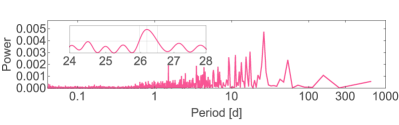
Figure 19.— A periodogram of the Kepler light curve, after transits were removed. The maximum power occurs at a period of $\mathord{\sim}26.2$ days, or half of the orbital period of the inner planet.

10. Summary

We have presented herein the discovery of the Kepler-432 planetary system, consisting of two giant planets orbiting a red giant star, and a faint visual companion that is probably a physically bound M dwarf with an orbital separation of at least $750$ AU. The inner planet ($P=52.5$ days) transits the star, allowing a more detailed study of its properties.

An asteroseismic analysis of the host star allows precise measurements of the stellar mass, radius, age, and spin axis inclination. This in turn leads to precise planetary properties, especially for the transiting inner planet. N-body simulations have helped constrain the properties of the outer planet by invoking stability arguments to rule out a large fraction of orbital solutions.

Kepler-432b is among the most massive transiting planets orbiting any type of star. Furthermore, it is not highly irradiated like many of the more common short-period transiting planets, experiencing only $\mathord{\sim}20\%$ of the insolation that a $3$-day hot Jupiter orbiting a Sun-like star would receive. This makes it an interesting benchmark for interior models, and a good test of planetary inflation at moderate insolation. It appears to be slightly inflated compared to the models, but is marginally consistent with having no core (or a small core) of heavy elements.

The eccentricities of both planets are high, which is suggestive of migration through multi-body interactions. Puzzlingly, the transiting planet is likely well aligned with the stellar spin, which is not an expected property of systems that have experienced such interactions. However, subsequent tidal or magnetic interaction with the host star may reconcile the two results. We find that because of the large stellar radius and planetary mass, the tidal dissipation timescale of the system is similar to that of hot Jupiters that are well-aligned. Those planets are thought to be well-aligned due to reorientation of the angular momenta after the initial inward migration; we conclude that the same process that realigns hot Jupiter systems may have also realigned this system, despite its long period.

Under the assumption that the star and planet are interacting strongly enough to realign the stellar spin, we searched for evidence of this interaction in the Kepler photometry. The star is photometrically quiet on long timescales, which allowed us to detect a low amplitude brightening soon after periastron. We conclude that the most likely explanation is a bright spot excited (either tidally or magnetically) by the planet during its close approach to the stellar photosphere. This evidence for ongoing SPI further supports the obliquity realignment scenario.

Finally, we note that Kepler-432b is an outlier among giant planets orbiting giant stars. It is one of only three such planets orbiting within $0.5$ AU of its host star. Either it is intrinsically rare, or it is one of a more common class of planets orbiting interior to $1$ AU that get destroyed relatively quickly once the star reaches the red giant branch. Given that Kepler-432 has only recently started its ascent up the RGB—most red giants are in a more advanced evolutionary state—and there is already evidence for SPI, it is plausible that many more red giants initially hosted planets similar to Kepler-432b that have subsequently been engulfed. Further investigation of this group of planets will provide more clarity and ultimately have strong implications for giant planet formation around intermediate and high mass stars, which are more difficult to study on the main sequence because of their high temperatures and rapid rotation.

References

- Aerts et al. (2010) Aerts, C., Christensen-Dalsgaard, J., & Kurtz, D. W. 2010, Asteroseismology (Springer)
- Aizenman et al. (1977) Aizenman, M., Smeyers, P., & Weigert, A. 1977, A&A, 58, 41
- Albrecht et al. (2012) Albrecht, S., Winn, J. N., Johnson, J. A., et al. 2012, ApJ, 757, 18
- Appourchaux et al. (2012) Appourchaux, T., Chaplin, W. J., García, R. A., et al. 2012, A&A, 543, 54
- Barclay et al. (2015) Barclay, T., Endl, M., Huber, D., et al. 2015, ApJ, 800, 46
- Barnes et al. (2011) Barnes, J. W., Linscott, E., & Shporer, A. 2011, ApJS, 197, 10
- Basu et al. (2010) Basu, S., Chaplin, W. J., & Elsworth, Y. 2010, ApJ, 710, 1596
- Batalha et al. (2013) Batalha, N. M., Rowe, J. F. , Bryson, S. T., et al. 2013, ApJS, 204, 24
- Beck et al. (2012) Beck, P. G., Montalban, J., Kallinger, T., et al. 2012, Nature, 481, 55
- Beck et al. (2014) Beck, P. G., Hambleton, K., Vos, J., et al. 2014, A&A, 564, 36
- Bedding et al. (2011) Bedding, T. R., Mosser, B., Huber, D. et al. 2011, Nature, 471, 608
- Belkacem et al. (2011) Belkacem, K., Goupil, M. J., Dupret, M. A., et al. 2011, A&A, 530, 142
- Benomar et al. (2014) Benomar, O., Masuda, K., Shibahashi, H., & Suto, Y. 2014, PASJ, 66, 94
- Berta et al. (2012) Berta, Z. K., Charbonneau, D., Désert, J.-M., et al. 2012, ApJ, 747, 35
- Borucki et al. (2010) Borucki, W. J., Koch, D., Basri, G., et al. 2010, Sci, 327, 977
- Bowler et al. (2010) Bowler, B. P., Johnson, J. A., Marcy, G. W., Henry, G. W., et al. 2010, ApJ, 709, 396
- Brandão et al. (2011) Brandão, I. M., Doğan, G., Christensen-Dalsgaard, J., et al. 2011, A&A, 527, 37
- Bressan et al. (2012) Bressan, A., Marigo, P., Girardi, L., et al. 2012, MNRAS, 427, 127
- Brown et al. (2011) Brown, T. M., Latham, D. W., Everett, M. E., & Esquerdo, G. A. 2011, AJ, 142, 112
- Buchhave et al. (2010) Buchhave, L. A., Bakos, G. Á., Hartman, J. D., et al. 2010, ApJ, 720, 1118
- Buchhave et al. (2012) Buchhave, L. A., Latham, D. W., Johansen, A., et al. 2012, Natur, 486, 375
- Buchhave et al. (2014) Buchhave, L. A., Bizzarro, M., Latham, D. W., et al. 2014, Natur, 509, 593
- Buchner et al. (2014) Buchner, J., Georgakakis, A., Nandra, K., et al. 2014, A&A, 564, 125
- Casella & George (1992) Casella, G., & George, E. I. 1992, American Statistician, 46, 3
- Chaplin et al. (2013) Chaplin, W. J., Sanchis-Ojeda, R., Campante, T. L., et al. 2013, ApJ, 766, 101
- Chaplin et al. (2014) Chaplin, W. J., Basu, S., Huber, D., et al. 2014, ApJS, 210, 1
- Charbonneau et al. (2002) Charbonneau, D., Brown, T. M., Noyes, R. W., & Gilliland, R. L. 2002, ApJ, 568, 377
- Chen et al. (2014) Chen, Y., Girardi, L., Bressan, A., et al. 2014, MNRAS, 444, 2525
- Christensen-Dalsgaard (2008a) Christensen-Dalsgaard, J. 2008a, Ap&SS, 316, 13
- Christensen-Dalsgaard (2008b) Christensen-Dalsgaard, J. 2008b, Ap&SS, 316, 113
- Ciceri et al. (2015) Ciceri, S., Lillo-Box, J., Southworth, J., et al. 2015, A&A, 573, L5
- Collier Cameron et al. (2010) Collier Cameron, A., Bruce, V. A., Miller, G. R. M., et al. 2010, MNRAS, 403, 151
- Dawson & Johnson (2012) Dawson, R. I., & Johnson, J. A. 2012, ApJ, 756, 122
- Dawson (2014) Dawson, R. I. 2014, ApJL, 790, 31
- de Rosa et al. (2014) de Rosa, R. J., Patience, J., Wilson, P. A., et al. 2014, MNRAS, 437, 1216
- Désert et al. (2011) Désert, J.-M., Charbonneau, D., Demory, B.-O., Ballard, S., et al. 2011, ApJS, 197, 14
- Djupvik & Andersen (2010) Djupvik, A. A., & Andersen, J. 2010, in Highlights of Spanish Astrophysics V, ed. J. M. Diego, L. J. Goicoechea, J. I. González-Serrano, & J. Gorgas (Berlin: Springer), p. 211
- Döllinger et al. (2009) Döllinger, M. P., Hatzes, A. P., Pasquini, L., Guenther, E. W., & Hartmann, M. 2009, A&A, 505, 1311
- Fabrycky & Tremaine (2007) Fabrycky, D., & Tremaine, S. 2007, ApJ, 669, 1298
- Feroz et al. (2009) Feroz, F., Hobson, M. P., & Bridges, M.. 2009, MNRAS, 398, 1601
- Feroz et al. (2013) Feroz, F., Hobson, M. P., Cameron, E., & Pettitt, A. N. 2013, arXiv:1306.2144
- Fortney et al. (2007) Fortney, J. J., Marley, M. S., Barnes, J. W. 2007, ApJ, 659, 1661
- Frandsen & Lindberg (1999) Frandsen, S., & Lindberg, B. 1999, Astrophysics with the NOT, ed. H. Karttunen & V. Piirola (Piikkio: Univ. Turku), 71
- Fűrész (2008) Fűrész, G. 2008, Ph.D. thesis, University of Szeged, Hungary
- Gai et al. (2011) Gai, N., Basu, S., Chaplin, W. J., & Elsworth, Y. 2011, ApJ, 730, 63
- Girardi et al. (2005) Girardi, L., Groenewegen, M. A. T., Hatziminaoglou, E., & da Costa, L. 2005, A&A, 436, 895
- Gizon & Solanki (2003) Gizon, L., & Solanki, S. K. 2003, ApJ, 589, 1009
- Goldreich & Tremaine (1980) Goldreich, P., & Tremaine, S. 1980, ApJ, 241, 425
- Handberg & Campante (2011) Handberg, R., & Campante, T. L. 2011, A&A, 527, 56
- Handberg & Lund (2014) Handberg, R., & Lund, M. N. 2014, MNRAS, 445, 2698
- Hastings (1970) Hastings, W. H. 1970, Biometrika, 57, 97
- Horch et al. (2010) Horch, E. P., Falta, D., Anderson, L. M., et al. 2010, AJ, 139, 205
- Houdek et al. (1999) Houdek, G., Balmforth, N. J., Christensen-Dalsgaard, J., & Gough, D. O. 1999, A&A, 351, 582
- Howell et al. (2011) Howell, S. B., Everett, M. E., Sherry, W., et al. 2011, AJ, 142, 19
- Huber et al. (2013a) Huber, D., Chaplin, W. J., Christensen-Dalsgaard, J., et al. 2013a, ApJ, 767, 127
- Huber et al. (2013b) Huber, D., Carter, J. A., Barbieri, M., et al. 2013b, Sci, 342, 331
- Ida & Lin (2005) Ida, S., & Lin, D. N. C 2005, ApJ, 626, 1045
- Jackson et al. (2008) Jackson, B., Greenberg, R., & Barnes, R. 2008, ApJ, 678, 1396
- Jiang et al. (2011) Jiang, C., Jiang, B. W., Christensen-Dalsgaard, J., et al. 2011, ApJ, 742, 120
- Johnson et al. (2007) Johnson, J. A., Fischer, D. A., Marcy, G. W., Wright, J. T., et al. 2007, ApJ, 665, 785
- Johnson et al. (2010) Johnson, J. A., Aller, K. M., Howard, A. W., & Crepp, J. R. 2010, PASP, 122, 905
- Johnson et al. (2011) Johnson, J. A., Clanton, C., Howard, A. W., Bowler, B. P., et al. 2011, ApJS, 197, 26
- Johnson et al. (2014) Johnson, M. C., Cochran, W. D., Albrecht, S., et al. 2014, ApJ, 790, 30
- Jones et al. (2014) Jones, M. I., Jenkins, J. S., Bluhm, P., Rojo, P., & Melo, C. H. F. 2014, A&A, 566, 113
- Juric & Tremaine (2008) Juric, M., & Tremaine, S. 2008, ApJ, 686, 603
- Kallinger et al. (2010) Kallinger, T., Weiss, W. W., Barban, C., et al. 2010, A&A, 509, 77
- Kipping (2008) Kipping, D. M. 2008, MNRAS, 389, 1383
- Kipping (2010) Kipping, D. M. 2010, MNRAS, 408, 1758
- Kipping et al. (2012) Kipping, D. M., Dunn, W. R., Jasinski, J. M., & Manthri, V. P. 2012, MNRAS, 421, 1166
- Kipping et al. (2013) Kipping, D. M., Hartman, J., Buchhave, L. A., et al. 2013, ApJ, 770, 101
- Kipping (2013a) Kipping, D. M. 2013a, MNRAS, 435, 2152
- Kipping (2013b) Kipping, D. M. 2013b, MNRAS, 434, 51
- Kipping (2014a) Kipping, D. M. 2014a, MNRAS, 440, 2164
- Kipping (2014b) Kipping, D. M. 2014b, MNRAS, 444, 2263
- Kjeldsen & Bedding (1995) Kjeldsen, H., & Bedding, T. R. 1995, A&A, 293, 87
- Kjeldsen et al. (2008) Kjeldsen, H., Bedding, T. R., & Christensen-Dalsgaard, J. 2008, ApJL, 683, 175
- Knutson et al. (2008) Knutson, H. A., Charbonneau, D., Allen, L. E., et al. 2008, ApJ, 673, 526
- Koch et al. (2010) Koch, D. G., Borucki, W. J., Basri, G., et al. 2010, ApJL, 713, 79
- Konstantinova-Antova et al. (2013) Konstantinova-Antova, R., Aurére, M., Charbonnel, C., Wade, G., et al. 2013, BlgAJ, 19, 14
- Kraft (1967) Kraft, R. P. 1967, ApJ, 150, 551
- Kurucz (1992) Kurucz, R. L. 1992, IAUS, 149, 225
- Lillo-Box et al. (2014a) Lillo-Box, J., Barrado, D., Moya, A., et al. 2014a, A&A, 562, 109
- Lillo-Box et al. (2014b) Lillo-Box, J., Barrado, D., Henning, T., et al. 2014b, A&A, 568, L1
- Lin & Papaloizou (1986) Lin, D. N. C., & Papaloizou, J. 1986, ApJ, 309, 846
- Lomb (1976) Lomb, N. R. 1976, Ap&SS, 39, 447
- Lovis & Mayor (2007) Lovis, C., & Mayor, M. 2007, A&A, 472, 657
- Lund et al. (2014) Lund, M. N., Lundkvist, M., Silva Aguirre, V., et al. 2014, A&A, 570, 54
- Mandel & Agol (2002) Mandel, K., & Agol, E. 2002, ApJL, 580, 171
- Mandushev et al. (2005) Mandushev, G., Torres, G., Latham, D. W., et al. 2005, ApJ, 621, 1061
- Mathur et al. (2011) Mathur, S., Hekker, S., Trampedach, R., et al. 2011, ApJ, 741, 119
- McLaughlin (1924) McLaughlin, D. B. 1924, ApJ, 60, 22
- Metcalfe et al. (2010) Metcalfe, T. S., Monteiro, M. J. P. F. G., Thompson, M. J., et al. 2010, ApJ, 723, 1583
- Metropolis et al. (1953) Metropolis, N., Rosenbluth, A. W., Rosenbluth, M. N., et al. 1953, JhPh, 21, 1087
- Mosser et al. (2012a) Mosser, B., Goupil, M. J., Belkacem, K., et al. 2012a, A&A, 548, 10
- Mosser et al. (2012b) Mosser, B., Goupil, M. J., Belkacem, K., et al. 2012b, A&A, 540, 143
- Naoz et al. (2012) Naoz, S., Farr, W. M., & Rasio, F. A. 2012, ApJL, 754, 36
- Nidever et al. (2002) Nidever, D. L., Marcy, G. W., Butler, P. R., et al. 2002, ApJS, 141, 503
- Nutzman et al. (2011) Nutzman, P. A., Fabrycky, D. C., & Fortney, J. J. 2011, ApJL, 740, 10
- Ortiz et al. (2015) Ortiz, M., Gandolfi, D., Reffert, S., et al. 2015, A&A, 573, L6
- Paxton et al. (2013) Paxton, B., Cantiello, M., Arras, P., et al. 2013, ApJS, 208, 4
- Payne et al. (2013) Payne, M. J., Deck, K. M., Holman, M. J., & Perets, H. B. 2013, ApJ, 775, 44
- Petrovich (2014) Petrovich, C. 2014, ApJ, submitted, arXiv:1409.8296
- Poppenhaeger et al. (2013) Poppenhaeger, K., Schmitt, J. H. M. M., & Wolk, S. J. 2013, ApJ, 773, 62
- Queloz et al. (2001) Queloz, D., Henry, G. W., Sivan, J. P., et al. 2001, A&A, 379, 279
- Quinn et al. (2014) Quinn, S. N., White, R. J., Latham, D. W., et al. 2014, ApJ, 787, 27
- Raghavan et al. (2010) Raghavan, D., McAlister, H. A., Henry, T. J., et al. 2010, ApJS, 190, 1
- Rasio & Ford (1996) Rasio, F. A., & Ford, E. B. 1996, Sci, 274, 954
- Rauch & Holman (1999) Rauch, K. P., & Holman, M. 1999, AJ, 117, 1087
- Rossiter (1924) Rossiter, R. A. 1924, ApJ, 60, 15
- Saar & Donahue (1997) Saar, S. H., & Donahue, R. A. 1997, ApJ, 485, 319
- Sanchis-Ojeda et al. (2011) Sanchis-Ojeda, R., Winn, J. N., Holman, M. J., Carter, J. A., et al. 2011, ApJ, 733, 127
- Sato et al. (2008) Sato, B., Izumiura, H., Toyota, E., Kambe, E., et al. 2008, PASJ, 60, 539
- Scargle (1982) Scargle, J. D., ApJ, 263, 835
- Schlafly & Finkbeiner (2011) Schlafly, E. F., & Finkbeiner, D. P. 2011, ApJ, 737, 103
- Schlegel et al. (1998) Schlegel, D. J., Finkbeiner, D.P., & Davis, M. 1998, ApJ, 500, 525
- Shkolnik et al. (2009) Shkolnik, E., Aigrain, S., Cranmer, S., et al. 2009, AIP Conf. Series 1094, Cool Stars, Stellar Systems, and the Sun, ed. E. Stempels (Melville, NY: AIP), 275
- Silva Aguirre et al. (2012) Silva Aguirre, V., Casagrande, L., Basu, S., et al. 2012, ApJ, 757, 99
- Silva Aguirre et al. (2014) Silva Aguirre, V., Ruchti, G. R., Hekker, S., et al. 2014, ApJ, 784, 16
- Skrutskie et al. (2006) Skrutskie, M. F., Cutri, R. M., Stiening, R., et al. 2006, AJ, 131, 1163
- Sliski & Kipping (2014) Sliski, D. H., & Kipping, D. M. 2014, ApJ, 788, 148
- Steffen et al. (2012) Steffen, J. H., Ragozzine, D., Fabrycky, D. C., et al. 2012, PNAS, 109, 7982
- Stello et al. (2008) Stello, D., Bruntt, H., Preston, H., & Buzasi, D. 2008, ApJ, 674, 53
- Stello et al. (2009) Stello, D., Chaplin, W. J., Bruntt, H., et al. 2009, ApJ, 700, 1589
- Stello et al. (2013) Stello, D., Huber, D., Bedding, T. R., et al. 2013, ApJ, 765, 41
- Strugarek et al. (2014) Strugarek, A., Brun, A. S., Matt, S. P., & Réville, V. 2014, ApJ, 795, 86
- Tingley et al. (2011) Tingley, B., Bonomo, A. S., & Deeg, H. J. 2011, ApJ, 726, 112
- Torres et al. (2005) Torres, G., Konacki, M., Sasselov, D. D., & Jha, S. 2005, ApJ, 619, 558
- Torres et al. (2011) Torres, G., Fressin, F., Batalha, N. M., et al. 2011, ApJ, 727, 24
- Torres et al. (2012) Torres, G., Fischer, D. A., Sozzetti, A., et al. 2012, ApJ, 757, 161
- Townsend & Teitler (2013) Townsend, R. H. D., & Teitler, S. A. 2013, MNRAS, 435, 3406
- Valsecchi & Rasio (2014) Valsecchi, F., & Rasio, F. A. 2014, ApJ, 786, 102
- van Cleve (2008) van Cleve, J. 2008, Kepler Instrument Handbook (available at http://archive.stsci.edu/kepler/)
- Van Eylen et al. (2014) Van Eylen, V., Lund, M. N., Silva Aguirre, V., et al. 2014, ApJ, 782, 14
- Weiss & Schlattl (2008) Weiss, A., & Schlattl, H. 2008, Ap&SS, 316, 99
- Winn et al. (2010) Winn, J. N., Fabrycky, D., Albrecht, S., & Johnson, J. A. 2010, ApJL, 718, 145
- Wu & Murray (2003) Wu, Y., & Murray, N. 2003, ApJ, 589, 605
- Wu & Lithwick (2011) Wu, Y., & Lithwick, Y. 2011, ApJ, 735, 109
- Zacharias et al. (2013) Zacharias, N., Finch, C. T., Girard, T. M., et al. 2013, AJ, 145, 44
- Zahn (1977) Zahn, J.-P. 1977, A&A, 57, 383