On the two-loop corrections to the Higgs masses in the NMSSM

Abstract

We discuss the impact of the two-loop corrections to the Higgs mass in the NMSSM beyond $O(\alpha_{S}(\alpha_{b}+\alpha_{t}))$. For this purpose we use the combination of the public tools SARAH and SPheno to include all contributions stemming from superpotential parameters. We show that the corrections in the case of a heavy singlet are often MSSM-like and reduce the predicted mass of the SM-like state by about 1 GeV as long as $\lambda$ is moderately large. For larger values of $\lambda$ the additional corrections can increase the SM-like Higgs mass. If a light singlet is present the additional corrections become more important even for smaller values of $\lambda$ and can even dominate the ones involving the strong interaction. In this context we point out that important effects are not reproduced quantitatively when only including $O((\alpha_{b}+\alpha_{t}+\alpha_{\tau})^{2})$ corrections known from the MSSM.

I Introduction

The discovery of the Higgs boson at the Large Hadron Collider (LHC) has completed the standard model (SM) of particle physics Chatrchyan:2012ufa ; Aad:2012tfa . However, there are some hints that the SM cannot be the final theory for particle physics: it does not provide a dark matter candidate, cannot explain the observed baryon asymmetry or neutrino masses, and suffers from the hierarchy problem. There are different options to solve all of these problems. Supersymmetry (SUSY) is still the most popular among them, see Ref. Nilles:1983ge ; Martin:1997ns and references therein. In the past the focus has mostly been on the minimal supersymmetric standard model (MSSM) but recently the interest in non-minimal SUSY models has grown, mainly for two reasons: (i) no hints for SUSY particles have so far been detected at the LHC; (ii) the observed Higgs mass of $m_{h}\simeq 125$ GeV is rather close to the upper limit of 132 GeV possible in the MSSM for moderate SUSY masses including three-loop corrections Feng:2013tvd ; Kant:2010tf . Together these lead to the question of how natural the MSSM is. The situation becomes significantly improved if a singlet superfield is added to the particle content of the MSSM: the interactions with the singlet can give a push to the Higgs mass at tree-level Ellwanger:2009dp ; Ellwanger:2006rm which reduces the necessary fine-tuning significantly BasteroGil:2000bw ; Dermisek:2005gg ; Ellwanger:2011mu ; Ross:2011xv ; Ross:2012nr ; Ross:2012nr ; Kaminska:2014wia . The NMSSM has a rich collider phenomenology Dreiner:2012ec and it has been shown recently that light singlinos could help to hide SUSY at the LHC Ellwanger:2014hia . The most studied singlet extension is the next-to-minimal supersymmetric standard model Ellwanger:2009dp which introduces a $\mathbb{Z}_{3}$ to forbid all dimensionful parameters in the superpotential.

To confront the NMSSM with the measured Higgs mass a precise calculation is necessary. Therefore, much effort has been expended on a full one-loop calculation in the $\overline{\mathrm{DR}}^{\prime}$-scheme Degrassi:2009yq ; Staub:2010ty as well as different on-shell schemes Ender:2011qh ; Graf:2012hh . At the two-loop level the dominant $\alpha_{S}(\alpha_{b}+\alpha_{t})$ have been available for a few years Degrassi:2009yq , but two-loop corrections involving only superpotential couplings such as Yukawa and singlet interactions have not been available so far. Up until now the state-of-the art codes to calculate the Higgs mass written specifically for the NMSSM are NMSPEC Ellwanger:2006rn , Next-to-Minimal SOFTSUSY Allanach:2001kg ; Allanach:2013kza ; Allanach:2014nba , and NMSSMCALC Baglio:2013iia . The first two codes use the known MSSM $(\alpha_{b}+\alpha_{t}+\alpha_{\tau})^{2}$ and $\alpha_{s}(\alpha_{t}+\alpha_{b})$ corrections, while NMSSMCALC includes only $(\alpha_{s}\alpha_{t})$ at two-loop. However, in Ref. Goodsell:2014bna an extension of the Mathematica package SARAH Staub:2008uz ; Staub:2009bi ; Staub:2010jh ; Staub:2012pb ; Staub:2013tta has been presented which can write a two-loop calculation for SPheno Porod:2003um ; Porod:2011nf of CP-even Higgs masses in models beyond the MSSM with a similar precision as known for the MSSM Brignole:2001jy ; Degrassi:2001yf ; Brignole:2002bz ; Dedes:2002dy ; Dedes:2003km . To be more precise, a lot of effort has been (and will be) made to take the Higgs mass precision in the MSSM beyond the effective potential Martin:2004kr ; Martin:2007pg ; Borowka:2014wla ; Degrassi:2014pfa , including RGE improvement and diagrammatic calculations. Advanced techniques are implemented in FeynHiggs Hahn:2013ria ; Heinemeyer:2007aq ; Hahn:2005cu ; Heinemeyer:1998yj .

This calculation is based on the effective potential approach and uses generic results presented in Ref. Martin:2001vx . In this work we discuss the importance of these ‘full’ two-loop calculations in the NMSSM, pointing out when it is not sufficient to use the known MSSM corrections. As explained later the calculation performed by SPheno/SARAH does not include corrections stemming from $g_{1}$ and $g_{2}$ but we will denote them nevertheless by ‘full’ for brevity since all corrections stemming from superpotential parameters are included. This corresponds to the precision of state of the art calculations widely used in the MSSM, with the possible exception of corrections to the mass of the $Z$ boson which feed into the determination of the electroweak scale.

We proceed as follows: in sec. II we fix our conventions and present details of the two-loop mass calculation. In sec. III we show the numerical impact of the full two-loop calculation before we conclude in sec. IV. The reader may refer to the appendix for some details of the calculation of the tree and one-loop Higgs mass matrices in our conventions; in particular, we describe there the treatment of the would-be Goldstone bosons, which provide some technical challenges for the calculation of the Higgs mass in the effective potential approach.

II Calculation of the Two-loop Higgs masses in the NMSSM

In this section we fix our notation and discuss the procedure for the calculations of the Higgs masses at two loops. Note that we shall focus throughout on the ‘NMSSM’ as the theory invariant under a $\mathbb{Z}_{3}$-symmetry, referring only briefly to more general variants.

II.1 Superpotential and soft SUSY breaking terms of the NMSSM

In the NMSSM, the particle content of the MSSM is extended by a gauge singlet superfield $\hat{S}$. We are using in the following the convention that all superfields are denoted by a ’hat’, the SUSY partners carry a ’tilde’ and the SM fields come without any decoration. All interactions in the superpotential consistent with an underlying $\mathbb{Z}_{3}$ symmetry are given by

$$W_{\rm{NMSSM}}=-\hat{H}_{u}\hat{Q}Y_{u}\hat{U}^{c}+\hat{H}_{d}\hat{Q}Y_{d}\hat{D}^{c}+\hat{H}_{d}\hat{L}Y_{e}\hat{E}^{c}+\lambda\hat{H}_{u}\hat{H}_{d}\hat{S}+\frac{1}{3}\kappa\hat{S}\hat{S}\hat{S}.$$ (1)

The corresponding soft-terms read

$$\mathscr{V}_{\rm SB,2} = m_{H_{u}}^{2}|H_{u}|^{2}+m_{H_{d}}^{2}|H_{d}|^{2}+m_{S}^{2}|S|^{2}+\tilde{Q}^{\dagger}m_{\tilde{Q}}^{2}\tilde{Q}+\tilde{L}^{\dagger}m_{\tilde{L}}^{2}\tilde{L}+\tilde{D}^{\dagger}m_{\tilde{D}}^{2}\tilde{D}+\tilde{U}^{\dagger}m_{\tilde{U}}^{2}\tilde{U}+$$ (2)

$$\hskip 28.45274pt+\frac{1}{2}\left(M_{1}\,\tilde{B}\tilde{B}+M_{2}\,\tilde{W}_{a}\tilde{W}^{a}+M_{3}\,\tilde{g}_{\alpha}\tilde{g}^{\alpha}+h.c.\right)$$

$$\mathscr{V}_{\rm SB,3} = -H_{u}\tilde{Q}T_{u}\tilde{U}^{\dagger}+H_{d}\tilde{Q}T_{d}\tilde{D}^{\dagger}+H_{d}\tilde{L}T_{e}\tilde{E}^{\dagger}+T_{\lambda}H_{u}H_{d}S+\frac{1}{3}T_{\kappa}SSS$$ (3)

After electroweak symmetry breaking (EWSB), the singlet is split into its CP even and odd component as well as a vacuum expectation value (VEV), just like the neutral parts of the Higgs doublets:

$$S = \frac{1}{\sqrt{2}}\left(\phi_{s}+i\sigma_{s}+v_{s}\right)\,,$$ (4)

$$H_{i}^{0} = \frac{1}{\sqrt{2}}\left(\phi_{i}+i\sigma_{i}+v_{i}\right)\hskip 28.45274pti=d,u\,.$$ (5)

We choose a phase convention such that all VEVs are real. The VEV of the singlet triggers effective $\mu$- and $B\mu$-terms

$$\mu_{\rm{eff}}=\frac{1}{\sqrt{2}}\lambda v_{s},\qquad B_{\mu,\rm{eff}}=\frac{1}{\sqrt{2}}T_{\lambda}v_{s}+\frac{1}{2}\kappa\lambda v_{s}^{2}.$$ (6)

We shall treat $\mu_{\rm{eff}}$ as an input parameter from which we extract $v_{s}$. The tree-level mass matrices for the neutral scalars and pseudoscalars are given in our notation in the appendix (eqs. (23,26), and the tadpole equations are given in equations (18 – 20). Throughout we shall make the choice of solving the three equations for $m^{2}_{H_{d}},m^{2}_{H_{u}}$ and $m^{2}_{S}$, leaving the input parameters to be

$$(\lambda,\mu_{\rm{eff}},T_{\lambda},T_{\kappa})$$

in addition to the parameters of the MSSM. It will sometimes be convenient in the following to define

$$T_{\lambda}\equiv\lambda A_{\lambda},\qquad T_{\kappa}\equiv\kappa A_{\kappa}.$$

We shall distinguish between two regimes of principal interest for the model: ones with a “heavy” singlet and ones with a “light” singlet, by which we mean respectively a singlet heavier than the standard-model-like Higgs, and of comparable or smaller mass.

II.2 Two-loop self-energies

The calculation of the two-loop self-energies is performed with the public tools SARAH and SPheno. The method applied by these tools is the one presented in Ref. Martin:2002wn : the effective potential is calculated at the two-loop level using the generic expressions of Ref. Martin:2001vx . The tadpole contributions and self-energies are calculated by taking the first and second derivative of the two-loop effective potential $V_{\text{eff}}^{(2)}$

$$\delta t^{(2)}_{i} = \frac{\partial V_{\text{eff}}^{(2)}}{\partial v_{i}}$$ (7)

$$\Pi_{h_{i}h_{j}}^{(2)}(0) = \frac{\partial^{2}V_{\text{eff}}^{(2)}}{\partial v_{i}\partial v_{j}}$$ (8)

with $i=d,u,s$. We give details of the tree-level mass matrices and further details of the procedure for calculating the loop-level masses in the appendix.

In SARAH/SPheno there are currently two possibilities to take the derivatives: one can numerically calculate the derivative of the entire potential; or one can take the derivative of the potential with respect to the masses analytically and numerically evaluate the derivatives of the masses and couplings with respect to the VEVs. Since the contributions to the two-loop Higgs mass for the NMSSM presented below are new there are no extant codes or calculations with which to compare the full results, and so we have compared the results for the two different methods to ensure that there was agreement. In addition, there is a third possible method of calculation based on a fully analytical diagrammatic approach to the Higgs mass calculation which will be presented elsewhere POLEInProgress , which has been implemented in SARAH/SPheno and will be made available in a future release. Since this is a rather independent calculation that does not rely on computing the effective potential itself the comparison with the other two methods is a non-trivial check; we have performed this and found excellent agreement.

Figure 1: Feynman diagrams contributing to $\alpha_{S}(\alpha_{b}+\alpha_{t})$ corrections in the effective potential at the two-loop level. The corrections involve SM fermions ($f_{i},f^{\prime}_{i}\equiv d_{i},u_{i},l_{i},\nu_{i}$) and SUSY sfermions ($\tilde{f}_{i},\tilde{f}_{i}^{\prime}\equiv\tilde{d}_{i},\tilde{u}_{i},\tilde{l}_{i},\tilde{\nu}_{i}$). A sum over all possible flavour combinations is assumed, but all CP and charge violating diagrams are not considered.

Figure 2: Feynman diagrams involving SM Yukawa couplings which contribute to the effective potential at the two-loop level. The corrections involve SM fermions ($f_{i},f^{\prime}_{i}\equiv d_{i},u_{i},l_{i},\nu_{i}$), SUSY sfermions ($\tilde{f}_{i},\tilde{f}_{i}^{\prime}\equiv\tilde{d}_{i},\tilde{u}_{i},\tilde{l}_{i},\tilde{\nu}_{i}$), neutralinos/charginos $\chi_{i}\equiv\tilde{\chi}^{0}_{i},\tilde{\chi}^{+}_{i}$, and Higgs particles $\phi_{i}\equiv h_{i},A_{i}^{0},H_{i}^{+}$. A sum over all possible flavour combinations is assumed, but all CP and charge violating diagrams are not considered.

Figure 3: Feynman diagrams contributing to $(\alpha_{\lambda}+\alpha_{\kappa})^{2}$ corrections to the effective potential at the two-loop level. These consist of the corrections from neutralinos/charginos $\chi_{i},\chi^{\prime}_{i}\equiv\tilde{\chi}^{0}_{i},\tilde{\chi}^{+}_{i}$, and Higgs particles $\phi_{i},\phi^{\prime}_{i}\equiv h_{i},A_{i}^{0},H_{i}^{+}$. A sum over all possible generations is assumed, but all CP and charge violating diagrams are not considered.

The calculation of $V_{\text{eff}}^{(2)}$ is performed in the gaugeless limit and includes all possible two-loop corrections except those involving the electroweak gauge couplings $g_{1}$ and $g_{2}$. We list the corresponding diagrams in Figs. 1–3. The corrections of $O(\alpha_{S}(\alpha_{t}+\alpha_{b}))$ stemming from the diagrams in Fig. 1 had already been calculated in the context of the NMSSM Degrassi:2009yq and the perfect agreement between the results obtained by SARAH/SPheno and those of Ref. Degrassi:2009yq was shown in Ref. Goodsell:2014bna . The classes of diagrams shown in Fig. 2 have so far only been calculated in the MSSM Brignole:2001jy ; Degrassi:2001yf ; Brignole:2002bz ; Dedes:2002dy ; Dedes:2003km but not in the NMSSM. Finally, contributions similar to Fig. 3 are completely absent in the MSSM in the limit $g_{1}=g_{2}=0$ but are present in the NMSSM, so these represent a novel contribution.

III Numerical Results

III.1 Numerical setup

For the numerical analysis we generated with SARAH 4.4.0 the Fortran code for SPheno which was compiled with SPheno 3.3.3. We applied by hand a few changes to that code to turn on/off different two-loop contributions individually. In addition, we included for comparison the $\alpha_{S}(\alpha_{t}+\alpha_{b})$ corrections from the NMSSM of Ref. Degrassi:2009yq as well as the MSSM corrections of Refs. Brignole:2001jy ; Degrassi:2001yf ; Brignole:2002bz ; Dedes:2002dy ; Dedes:2003km for all other contributions. All parameter scans have been performed with SSP Staub:2011dp .

III.2 Heavy singlet case with moderate $\lambda$

To test the importance of the two-loop corrections beyond $O(\alpha_{s}(\alpha_{t}+\alpha_{b}))$ we start with a parameter point in the constrained NMSSM. In this constrained setup, universal boundary conditions at the GUT scale are assumed:

$$M_{1}=M_{2}=M_{3}\equiv M_{1/2}$$

$$m_{\tilde{D}}^{2}=m_{\tilde{U}}^{2}=m_{\tilde{Q}}^{2}=m_{\tilde{E}}^{2}=m_{\tilde{L}}^{2}\equiv m_{0}^{2}\,{\bf 1}_{3}$$

$$T_{i}\equiv A_{0}Y_{i}\hskip 14.22636pti=u,d,e;\hskip 28.45274ptT_{\lambda}\equiv A_{\lambda}\lambda;\quad\hskip 28.45274pt\quad T_{\kappa}\equiv A_{\kappa}\kappa$$

$M_{1/2}$, $m_{0}$, $A_{0}$, $A_{\lambda}$ and $A_{\kappa}$ are defined at the unification scale, while $\lambda$, $\kappa$, $\mu_{\rm{eff}}$ and $\tan\beta=\frac{v_{u}}{v_{d}}$ are defined at the SUSY scale. As an example for the discussion in the following we pick the point fixed by

$$m_{0}=1.4~{}\text{TeV}\,\hskip 14.22636ptM_{1/2}=1.4~{}\text{TeV}\,\hskip 14.22636pt\tan\beta=2.9\,\hskip 14.22636ptA_{0}=-1.35~{}\text{TeV}\,\hskip 14.22636pt$$

$$\lambda=0.56\,\hskip 14.22636pt\kappa=0.33\,\hskip 14.22636ptA_{\lambda}=-390~{}\text{GeV}\,\hskip 14.22636ptA_{\kappa}=-280~{}\text{GeV}\,\hskip 14.22636pt\mu_{\rm{eff}}=200~{}\text{GeV}$$ (9)

The results for the Higgs masses for this point at different loop level and with different loop corrections are summarised in Tab 1. Note that it is in this case the second neutral scalar $h_{2}$ that is predominantly singlet in this case (about $96\%$); we find at two loops

$$\phi_{s}=0.09h_{1}-0.98h_{2}+0.17h_{3}.$$

In this case the mass of the mostly singlet scalar is of the order of $200$ GeV, yet it does not mix substantially with the lightest Higgs state – justifying this point as being labelled “heavy”.

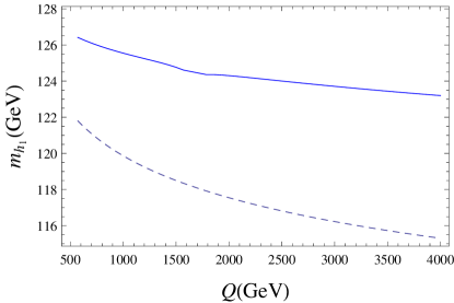
Figure 4: The light Higgs mass based on the parameter point of eq. 9 for a variation of the renormalisation scale $Q$. The dashed line is the one-loop prediction and the full line the two-loop one.

	Tree	one-loop	two-loop ($\alpha_{s}(\alpha_{b}+\alpha_{t})$)	full two-loop
$m_{h_{1}}$	93.8	117.6 (+ 25.4%)	126.1 (+7.2%)	124.7 (-1.1%)
$m_{h_{2}}$	214.5	209.2 (-2.4%)	209.2 ($\pm$ 0%)	208.7 (-0.2%)
$m_{h_{3}}$	555.5	541.9 (-2.4%)	542.3 (+0.1%)	541.4 (-0.2%)

Table 1: Higgs masses at tree-level, one-loop and two-loop for the parameter point of eq. (9) in GeV. Note that the second Higgs $h_{2}$ is mostly singlet-like, with the MSSM-like heavy Higgs being the heaviest ($h_{3}$).

At the two-loop level we distinguish two different cases: (i) including just $\alpha_{s}(\alpha_{t}+\alpha_{b})$ which had been calculated before for the NMSSM; (ii) the full NMSSM corrections calculated by SARAH/SPheno. We see in Tab. 1 that the tendencies are similar to the MSSM: while the corrections proportional to the strong interaction give a large positive shift to the Higgs masses, the corrections involving only superpotential couplings are negative for all three Higgs masses. If one compares these numbers with the same corrections in the CMSSM one sees that the two-loop corrections are dominated for this point by MSSM-like contributions: for the CMSSM point with $m_{0}=M_{1/2}=1.4$ TeV, $\tan\beta=2.9$, $\mu>0$ and $A_{0}=-1.35$ TeV, the contributions involving the strong-interaction cause a shift by +11.3 GeV, while the purely Yukawa corrections reduce the mass by -1.4 GeV.

To give an impression of the remaining uncertainty in the Higgs mass we show in Fig. 4 the calculated mass at one and two loops for a variation of the renormalisation scale $Q$. We see that the scale dependence is highly reduced at the two-loop level as expected. The average $M_{\text{SUSY}}=\sqrt{m_{\tilde{t}_{1}}m_{\tilde{t}_{2}}}$ of the stops (usually taken as the optimal renormalisation scale) is about $2$ TeV. The variation of the Higgs mass in the range $\frac{1}{2}M_{\text{SUSY}}$ and $2M_{\text{SUSY}}$ is $2.3$ GeV which can be taken as a rough indication of the remaining uncertainty.

The general picture of the importance of the loop corrections is also confirmed when we vary $\lambda$ and $\kappa$ as shown in Fig. 5.

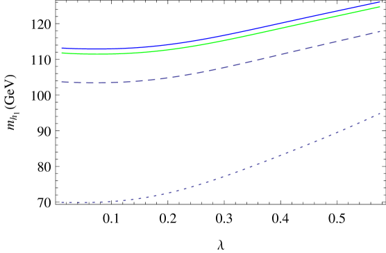
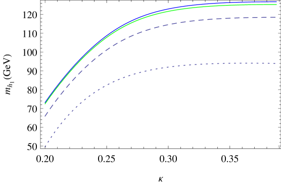
Figure 5: Light Higgs mass based on the parameter point of eq. 9 for a variation of $\lambda$ and $\kappa$. The Higgs mass is shown at tree-level (dotted line), one-loop (dashed line) and two-loops (full line). At two-loop level we distinguish between the $\alpha_{S}(\alpha_{b}+\alpha_{t})$ corrections (blue) and the full calculation in the NMSSM (green).

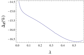
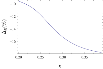
Figure 6: First row: the absolute size of the two-loop contributions beyond $O(\alpha_{S}(\alpha_{b}+\alpha_{t}))$ for the parameter variation shown in Fig. 5. Second row: the relative size of these corrections normalized to the $\alpha_{S}(\alpha_{b}+\alpha_{t})$ ones.

In general, the additional corrections are small compared to the corrections involving the strong interaction: for the above parameters the size of these corrections is 10%–20% of the size of the $\alpha_{s}$ corrections and dominated by the MSSM-like contributions. This also explains the very moderate dependence of the overall size of these corrections on the NMSSM specific parameters $\lambda$ and $\kappa$.

III.3 Heavy singlet with large $\lambda$

So far we concentrated on moderate values of $\lambda$, which are consistent with gauge coupling unification and do not cause a Landau pole below the unification scale. However, if one surrenders the condition of perturbativity up to the GUT scale larger values of $\lambda$ are possible. These so-called $\lambda$SUSY scenarios are popular because they predict very moderate values for the fine-tuning Hall:2011aa and have interesting phenomenological consequences SchmidtHoberg:2012yy ; SchmidtHoberg:2012ip . We consider in the following the point fixed by

$$\lambda=1.6\,\hskip 14.22636pt\kappa=1.6\,\hskip 14.22636pt\tan\beta=3\,\hskip 14.22636ptT_{\lambda}=600~{}\text{GeV}\,\hskip 14.22636ptT_{\kappa}=-2650~{}\text{GeV}\,\hskip 14.22636pt\mu_{\rm{eff}}=614~{}\text{GeV}\,\hskip 14.22636pt$$ (10)

All sfermion squared soft-masses are fixed to $2\cdot 10^{6}~{}\text{GeV}^{2}$, the gaugino masses are $M_{1}=200$ GeV, $M_{2}=400$ GeV, $M_{3}=2000$ GeV while all trilinear MSSM-like soft-terms are assumed to vanish. The corresponding masses are shown in Tab. 2. Again we find that the MSSM-heavy-Higgs-like state is the heaviest of the three neutral scalars, with the mostly-singlet neutral scalar having a mass of order $700$ GeV.

	Tree	one-loop	two-loop ($\alpha_{s}(\alpha_{b}+\alpha_{t})$)	full two-loop
$m_{h_{1}}$	144.8	122.6 (-15.3%)	126.5 (+3.2%)	128.0 (+1.2%)
$m_{h_{2}}$	713.2	745.9 (+4.6%)	745.8 (+0.0%)	747.9 (+0.3%)
$m_{h_{3}}$	1454.5	1421.1 (-2.3%)	1420.1 (-0.1%)	1420.3 (+0.0%)

Table 2: Higgs masses at tree-level, one-loop and two-loop for the parameter point of eq. (10). Again the second Higgs $h_{2}$ is mostly singlet-like, with the heavy Higgs $h_{3}$ being largely the MSSM heavy Higgs.

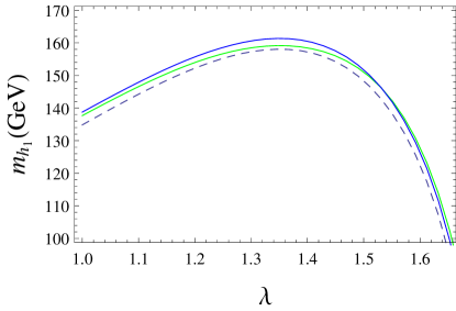
Figure 7: The light Higgs mass based on the parameter point of eq. 10 for a variation of $\lambda$. The colour and line coding is the same as in Fig. 5

We see that for this point all two-loop shifts to the lightest Higgs mass have the same sign, thus the NMSSM-specific corrections at some point dominate the ones of the MSSM. This is depicted in Fig. 7 where the light Higgs mass for a variation of $\lambda$ is shown: for $\lambda\simeq 1.5$ the sign of the corrections beyond $\alpha_{S}(\alpha_{t}+\alpha_{b})$ changes and those contributions become positive. This is depicted again on the left of Fig. 8 where the absolute size of the $\alpha_{S}(\alpha_{t}+\alpha_{b})$ and $(\alpha_{\lambda}+\alpha_{\kappa}+\alpha_{t}+\alpha_{b}+\alpha_{\tau})^{2}$ corrections are shown. On the right of Fig. 8 we zoom into the interesting range with a SM-like Higgs mass in the preferred range. In this plot we also show the expected mass if only MSSM-like corrections for the purely Yukawa part are included. One sees that this can give masses which are wrong by several GeV.

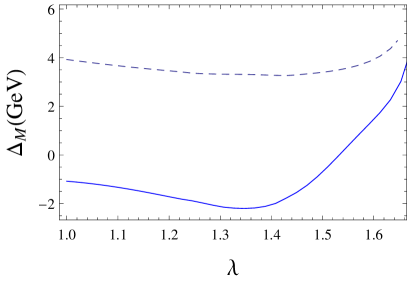
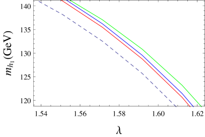
Figure 8: On the left: absolute size of the two-loop corrections $O(\alpha_{S}(\alpha_{t}+\alpha_{b}))$ (dashed) and $O((\alpha_{\lambda}+\alpha_{\kappa}+\alpha_{t}+\alpha_{b}+\alpha_{\tau})^{2})$ (full line). On the right: zoom into the interesting region of Fig. 7 with a SM-like Higgs state in the preferred range. The blue line is the mass including $\alpha_{S}(\alpha_{b}+\alpha_{t})$ corrections, the green line is the full calculation while the red line corresponds to MSSM-like corrections only for the Yukawa part.

III.4 Light singlet case

We have seen that in the case of a heavy singlet the additional two-loop contributions to the ones involving the strong interaction are MSSM-like. We discuss now the effects if a light singlet is present. For this purpose we consider the benchmark point BMP-A of Ref.Das:2014fha which has the interesting feature that all three scalars have masses below 200 GeV. The important parameter values are

$$\lambda=0.596\,\hskip 14.22636pt\kappa=0.596\,\hskip 14.22636ptT_{\lambda}=-27\ \text{GeV}\,\hskip 14.22636ptT_{\kappa}=-240~{}\text{GeV}\,\hskip 14.22636pt\mu_{\rm{eff}}=130~{}\text{GeV}$$

$$T_{t}=-3050~{}\text{GeV}\,\hskip 14.22636ptT_{b}=T_{\tau}=-1000~{}\text{GeV}\,\hskip 14.22636ptm^{2}_{\tilde{Q},33}=9.0\cdot 10^{5}~{}\text{GeV}^{2}\,\hskip 14.22636ptm^{2}_{\tilde{U},33}=1.05\cdot 10^{6}~{}\text{GeV}^{2}$$

(11)

We give in Tab.3 the values for the three scalar masses at the different loop levels. One sees here that in general the loop corrections to the SM-like Higgs, which is the second mass eigenstate, are less important than in the case of a heavy singlet because of the already enhanced tree-level mass. However, the interesting feature is that the one- and two-loop corrections can be of similar size and the most important corrections are the two-loop parts discussed here for the first time.

	Tree	one-loop	two-loop ($\alpha_{s}(\alpha_{b}+\alpha_{t})$)	full two-loop
$m_{h_{1}}$	19.4	67.8 (+249.5%)	74.5 (+9.9%)	74.2 (-0.4%)
$m_{h_{2}}$	122.7	123.5 (+0.7%)	124.3 (+0.6%)	123.3 (-0.8%)
$m_{h_{3}}$	177.4	188.2 (+6.1%)	192.7 (+2.3%)	191.1 (-0.8%)

Table 3: Higgs masses at tree-level, one-loop and two-loop for the parameter point of eq. (11).

To find a better understanding of the different effect, we depict the masses at tree-, one-loop and two-loop level for a variation of $\lambda$ in Fig. 9.

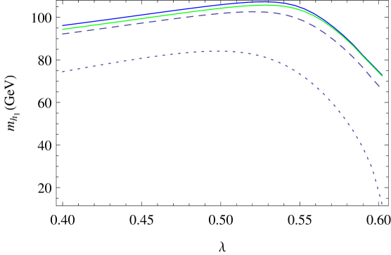
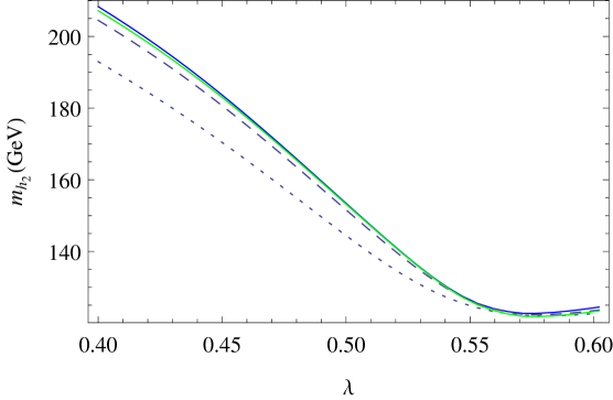
Figure 9: The two lightest Higgs masses based on the parameter point of eq. 11 for a variation of $\lambda$. The colour code is the same as in Fig. 5

One can see a very strong dependence of both masses on $\lambda$ which is however mainly caused by tree-level effects as indicated by the dotted line in Fig. 9: for small $\lambda$ the singlet is heavier than the doublet which causes a reduction of the tree-level mass due to mixing effects and the SM-like state is much too light. With increasing $\lambda$ the singlet becomes lighter and for $\lambda\simeq 0.55$ a level crossing takes place. The mixing with the lighter singlet as well as $F$-term contributions $\delta m_{h}\sim\frac{\lambda^{2}v^{2}}{2}\cos^{2}2\beta$ give a sizeable push to the SM-like Higgs state at tree-level. Thus, the interesting region is the one close to and above the level crossing and we zoom into this region in Fig. 10.

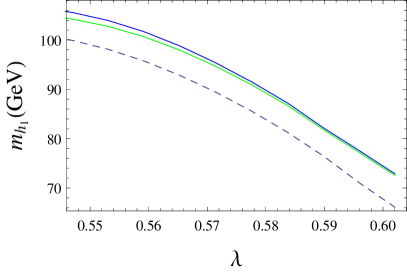
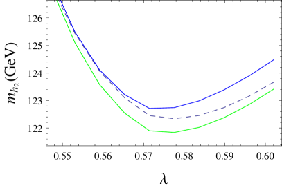
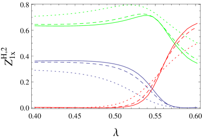
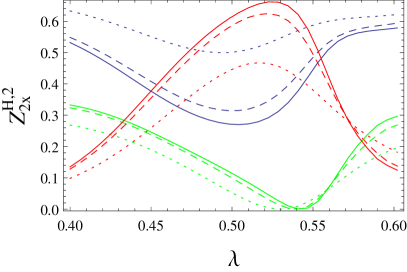
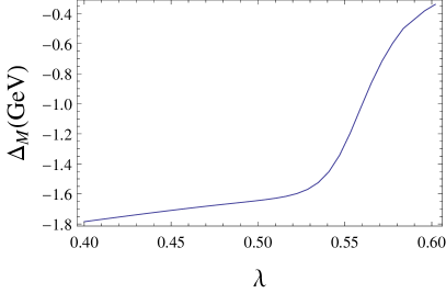
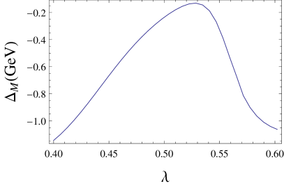
Figure 10: First row: zoom into the range $\lambda\in[0.4,0.6]$ of Fig. 9. The colour and line coding is the same as in Fig. 5. Second row: down- (blue), up- (green) and singlet- (red) fraction of the Higgs particle at tree-level (dotted), one-loop (dashed) and two-loop (full line). Third row: absolute size of the two-loop corrections not involving the strong interaction, for $m_{h_{1}}$ on the left and $m_{h_{2}}$ on the right.

We give in this Figure also the composition of the two light Higgs states as well as the absolute size of the full two-loop corrections compared to the $\alpha_{S}(\alpha_{t}+\alpha_{b})$ ones. One sees a strong correlation between the singlet fraction and the two-loop corrections not involving the strong interaction shown in the second and third row of Fig. 10: the absolute size of these corrections decreases with increasing singlet admixture. Thus, the main contribution to the two-loop masses despite the sizeable value of $\lambda$ is again caused by the MSSM-like corrections due to (s)quarks. Interestingly, for a light state below 80 GeV which is 60% singlet, the $\alpha_{S}(\alpha_{b}+\alpha_{t})$ can still give a sizeable push while the additional corrections nearly vanish. In contrast, for the SM-like particle and $\lambda>0.55$ the additional corrections discussed here can even dominate the strong corrections. Thus, in these cases the incomplete calculation would give the wrong picture that the two-loop corrections increase the Higgs mass.

Finally, we comment again on the approximation of using the known two-loop Yukawa corrections of the MSSM to the upper $2\times 2$ block of the scalar mass matrix. While, as we have shown above, this can sometimes be a good approximation for a MSSM-like state for moderate $\lambda$, we found in the previous subsections that this fails for larger $\lambda$. Another situation where this approximation gives wrong results is the case of light singlets as shown in Fig. 11.

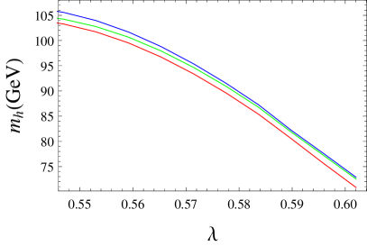
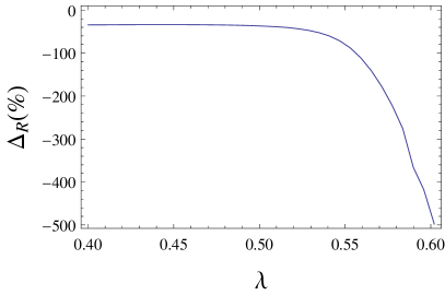
Figure 11: On the left: the lightest Higgs mass at two loops based on the parameter point of eq. 11 for a variation of $\lambda$. The blue line is the mass using only $\alpha_{s}(\alpha_{t}+\alpha_{b})$ corrections, the green line corresponds to our full calculation while the red line gives the obtained result when using the MSSM expressions for the pure Yukawa contributions. On the right we show the relative difference between the full corrections and the MSSM approximation.

We see in this Figure that the approximation to use the MSSM results for the purely Yukawa interactions roughly works for smaller values of $\lambda$ but becomes worse for increasing $\lambda$. For $\lambda\simeq 0.6$ this approximation predicts a change of about 2 GeV of the light Higgs mass compared to the full calculation of the NMSSM. This effect is mainly caused by the missing corrections to the $(1,3)$ and $(2,3)$ elements in the Higgs mass matrix. Since the corrections are negative for these entries and reduce the mixing between the doublets and singlet, the incomplete calculation predicts a mixing that is too large, which reduces the lighter mass eigenstate.

IV Discussion

We have examined the impact of the dominant two-loop corrections beyond $O(\alpha_{S}(\alpha_{t}+\alpha_{b}))$ in the NMSSM. The previously best approach was to use the $O(\alpha_{S}(\alpha_{t}+\alpha_{b}))$ routines for the NMSSM of Degrassi:2009yq and add the MSSM contributions for $O((\alpha_{t}+\alpha_{b}+\alpha_{\tau})^{2})$. We have found, as could be expected, that for small $\lambda$ this is a good approximation. It should also not be a surprise that it is a poor approximation when there is significant mixing between the singlet and the MSSM-like states, with an error of approximately $2$ GeV. On the other hand, we found that the approximation works up to somewhat large values of $\lambda$ when the singlet was heavier than the standard-model-like Higgs, although for $\lambda$ above around $1.5$ the full contribution has a different sign to the previous best approximation and so the correct result differs by a few GeV. To examine this more closely, let us consider the one-loop approximation for the Higgs mass including the stop corrections and leading $\lambda^{4}$ contributions (from singlet scalars and Higgsinos) in the decoupling limit of the effective potential approximation:

$$m_{h}^{2}\approx M_{Z}^{2}c_{\beta}^{2}+\frac{\lambda^{2}v^{2}s_{2\beta}^{2}}{2}+\frac{3}{2\pi^{2}}\frac{m_{t}^{4}}{v^{2}}\log\frac{m_{\tilde{t}_{1}}m_{\tilde{t}_{2}}}{m_{t}^{2}}+\frac{\lambda^{4}v^{2}}{32\pi^{2}}\log\frac{m_{\phi_{s}\phi_{s}}^{2}m_{\sigma_{s}\sigma_{s}}^{2}}{(4\kappa^{2}\mu_{\rm{eff}}^{2}/\lambda^{2})^{2}}.$$ (12)

We see at one loop:

1. As is well-known, for small $\tan\beta$ the tree-level mass is larger than in the MSSM, reducing the impact of radiative corrections.

2. The contributions from the singlet will typically be smaller than those of the stops unless we have a large $\lambda$, or $m_{\phi_{s}\phi_{s}}$ much larger than the stop mass.

3. Moreover, to obtain a substantial contribution from the singlets requires a large splitting between the singlet mass and the Higgsino mass $\mu_{\rm{eff}}$.

Now, in the NMSSM (respecting a $\mathbb{Z}_{3}$ symmetry) it is difficult to obtain a large value for the physical singlet mass, and moreover to split it from the Higgsinos. To see this, consider the large $v_{s}$ limit of the potential, where

$$V\simeq \frac{1}{2}m_{S}^{2}v_{s}^{2}+\frac{1}{3\sqrt{2}}\kappa A_{\kappa}v_{s}^{3}+\frac{1}{4}\kappa^{2}v_{s}^{4}.$$ (13)

This yields

$$m_{\phi_{s}\phi_{s}}^{2}\simeq \frac{\kappa}{\lambda}A_{\kappa}\mu_{\rm{eff}}+4\mu_{\rm{eff}}^{2}\left(\frac{\kappa}{\lambda}\right)^{2},\qquad m_{\sigma_{s}\sigma_{s}}^{2}\simeq-3\frac{\kappa}{\lambda}A_{\kappa}\mu_{\rm{eff}}.$$ (14)

However,

$$\mu_{\rm{eff}}\simeq \frac{\lambda}{4\kappa}\big{(}-A_{\kappa}+\sqrt{A_{\kappa}^{2}-8m_{S}^{2}}\big{)}.$$ (15)

We find that for a stable vacuum we require $A_{\kappa}^{2}\gtrsim 9m_{S}^{2}$ and therefore $\mu_{\rm{eff}}\sim-\frac{\lambda}{4\kappa}A_{\kappa}$, giving

$$m_{\phi_{s}\phi_{s}}^{2}\simeq 4\left(\frac{\kappa^{2}}{\lambda^{2}}\right)\mu_{\rm{eff}}\sqrt{A_{\kappa}^{2}-8m_{S}^{2}}<4\left(\frac{\kappa^{2}}{\lambda^{2}}\right)\mu_{\rm{eff}}^{2},\qquad m_{\sigma_{s}\sigma_{s}}^{2}\simeq 12\frac{\kappa^{2}}{\lambda^{2}}\mu_{\rm{eff}}^{2}.$$ (16)

Hence to obtain a large hierarchy between the singlets and the singlino is not possible at tree level. There is also a similar contribution proportional to $v^{2}\lambda^{4}$ from the heavy Higgs and the higgsinos, which then requires a hierarchy between the heavy higgs and $\mu_{\rm{eff}}$, which is similarly constrained. We therefore expect these observations for the heavy singlet limit to apply roughly at two loops, because the supersymmetric mass for the singlet is of the same order as the supersymmetry-breaking contribution.

In summary, we have examined the full two-loop corrections to the Higgs masses (calculated in the “gaugeless limit” where gauge couplings of broken gauge groups are ignored) in the NMSSM and compared them to the approximations previously available. The new corrections implemented in SARAH/SPheno are essential to obtain an accurate calculation of the Higgs mass in the NMSSM when the values of $\lambda$ are significant and/or there is substantial mixing between the singlet scalar and the MSSM-like Higgses. It would be interesting, however, to explore other singlet extensions where the quantum effects could be even more significant – for example the general NMSSM with a large $\lambda$, which would allow a genuinely large singlet scalar mass with a splitting between the scalar and Higgsinos. This can be done now by an interested reader since the codes SARAH and SPheno are publically available at HepForge (http://sarah.hepforge.org/, http://spheno.hepforge.org/) and SARAH includes several additional singlet extensions in addition to the NMSSM.

Appendix A Higgs sector of the NMSSM

A.1 Minimum Conditions of the Vacuum

At tree level, the tadpole equations (the minimum conditions for the vacuum) are given by

$$T_{i}=\frac{\partial V}{\partial v_{i}}\Big{|}_{\phi_{i}=0,\sigma_{i}=0}=0$$ (17)

with

$$\frac{\partial V}{\partial\phi_{d}} =m_{H_{d}}^{2}v_{d}+\frac{1}{8}\Big{(}g_{1}^{2}+g_{2}^{2}\Big{)}v_{d}\Big{(}v_{d}^{2}-v_{u}^{2}\Big{)}+\frac{1}{2}\Big{(}v_{d}\Big{(}v_{s}^{2}+v_{u}^{2}\Big{)}|\lambda|^{2}-v_{s}^{2}v_{u}\Re(\kappa\lambda^{*})-\sqrt{2}v_{s}v_{u}{\Re\Big{(}T_{\lambda}\Big{)}}\Big{)}$$ (18)

$$\frac{\partial V}{\partial\phi_{u}} =m_{H_{u}}^{2}v_{u}+\frac{1}{8}\Big{(}g_{1}^{2}+g_{2}^{2}\Big{)}v_{u}\Big{(}v_{u}^{2}-v_{d}^{2}\Big{)}+\frac{1}{2}\Big{(}\Big{(}v_{d}^{2}+v_{s}^{2}\Big{)}v_{u}|\lambda|^{2}-v_{d}v_{s}^{2}\Re(\kappa\lambda^{*})-\sqrt{2}v_{d}v_{s}{\Re\Big{(}T_{\lambda}\Big{)}}\Big{)}$$ (19)

$$\frac{\partial V}{\partial\phi_{s}} =m_{S}^{2}v_{s}-v_{d}v_{s}v_{u}\Re(\lambda\kappa^{*})+v_{s}^{3}|\kappa|^{2}+\frac{1}{2}\Big{(}v_{s}(v_{d}^{2}+v_{u}^{2})|\lambda|^{2}+\sqrt{2}\Big{(}-v_{d}v_{u}\Re(T_{\lambda})+v_{s}^{2}\Re(T_{\kappa})\Big{)}\Big{)}$$ (20)

All parameters in these equations are taken to be running $\overline{\mathrm{DR}}^{\prime}$ Jack:1994rk parameters at the renormalisation scale $Q$. In this context the VEVs $v_{d}$ and $v_{u}$ are derived from the running $Z$-boson mass $m_{Z}(Q)$ of the $Z$-boson. For more details of this approach we refer to Ref. Pierce:1996zz .

The tadpole equations receive finite corrections at loop level. We calculate the one- and two-loop shifts denoted as $\delta t^{(1)}_{i}$ and $\delta t^{(2)}_{i}$, and demand that the sum of all orders vanishes

$$T_{i}+\delta t^{(1)}_{i}+\delta t^{(2)}_{i}=0\qquad{\rm for}\quad i=d,u,s.$$ (21)

The calculation of the corrections at one-loop is discussed in detail in Ref. Staub:2010ty . Details about the two-loop contributions are given in the text in sec. II.2.

In our analysis we solve eqs. (21) for the soft SUSY breaking masses of the Higgs doublets and the singlet: $m^{2}_{H_{d}},m^{2}_{H_{u}}$, and $m^{2}_{S}$.

A.2 Masses of the Higgs bosons

A.2.1 Tree-level scalar masses

The tree-level mass matrices for the CP-even Higgs bosons bosons are calculated from the scalar potential via

$$m^{2,h}_{T,ij}=\frac{\partial^{2}V}{\partial\phi_{i}\partial\phi_{j}}\Bigg{|}_{\phi_{k}=0,\sigma_{k}=0},\hskip 56.9055pt$$ (22)

with $i,j=1,2,3=u,d,s$. The matrix is symmetric and the entries read

$$m_{\phi_{d}\phi_{d}} =\frac{1}{2}\Big{(}v_{s}^{2}+v_{u}^{2}\Big{)}|\lambda|^{2}+\frac{1}{8}\Big{(}g_{1}^{2}+g_{2}^{2}\Big{)}\Big{(}3v_{d}^{2}-v_{u}^{2}\Big{)}+m_{H_{d}}^{2}$$

$$m_{\phi_{d}\phi_{u}} =\frac{1}{4}\Big{(}-2\sqrt{2}v_{s}{\Re\Big{(}T_{\lambda}\Big{)}}+\Big{(}4v_{d}v_{u}\lambda-v_{s}^{2}\kappa\Big{)}\lambda^{*}-v_{s}^{2}\lambda\kappa^{*}\Big{)}-\frac{1}{4}\Big{(}g_{1}^{2}+g_{2}^{2}\Big{)}v_{d}v_{u}$$

$$m_{\phi_{u}\phi_{u}} =\frac{1}{2}\Big{(}v_{d}^{2}+v_{s}^{2}\Big{)}|\lambda|^{2}-\frac{1}{8}\Big{(}g_{1}^{2}+g_{2}^{2}\Big{)}\Big{(}-3v_{u}^{2}+v_{d}^{2}\Big{)}+m_{H_{u}}^{2}$$

$$m_{\phi_{d}\phi_{s}} =-\frac{1}{\sqrt{2}}v_{u}{\Re\Big{(}T_{\lambda}\Big{)}}+v_{s}\Big{(}\Big{(}-\frac{1}{2}v_{u}\kappa+v_{d}\lambda\Big{)}\lambda^{*}-\frac{1}{2}v_{u}\lambda\kappa^{*}\Big{)}$$

$$m_{\phi_{u}\phi_{s}} =\frac{1}{2}\Big{(}-v_{d}\Big{(}\sqrt{2}{\Re\Big{(}T_{\lambda}\Big{)}}+v_{s}\lambda\kappa^{*}\Big{)}-v_{s}\Big{(}-2v_{u}\lambda+v_{d}\kappa\Big{)}\lambda^{*}\Big{)}$$

$$m_{\phi_{s}\phi_{s}} =\frac{1}{2}\Big{(}2\sqrt{2}v_{s}{\Re\Big{(}T_{\kappa}\Big{)}}+\Big{(}6v_{s}^{2}\kappa-v_{d}v_{u}\lambda\Big{)}\kappa^{*}+\Big{(}\Big{(}v_{d}^{2}+v_{u}^{2}\Big{)}\lambda-v_{d}v_{u}\kappa\Big{)}\lambda^{*}\Big{)}+m_{S}^{2}$$ (23)

This matrix is diagonalised by a rotation matrix $Z^{H}$ and the relation

$$Z^{H}m^{2,h}Z^{H,T}=m^{2,h}_{\mathrm{diag}}\,.$$ (24)

holds. The three eigenvalues of $m^{2,h}_{T}$ correspond to three physical mass eigenstates with masses $m_{h_{1}}$, $m_{h_{2}}$, $m_{h_{3}}$ which are ordered by their mass.

A.2.2 Tree-level pseudo-scalar masses

Similarly, the mass matrix of the CP even states is calculated via

$$m^{2,A}_{T,ij}=\frac{\partial^{2}V}{\partial\sigma_{i}\partial\sigma_{j}}\Bigg{|}_{\phi_{k}=0,\sigma_{k}=0},\hskip 56.9055pt$$ (25)

and one finds

$$m_{\sigma_{d}\sigma_{d}} =\frac{1}{2}\Big{(}v_{s}^{2}+v_{u}^{2}\Big{)}|\lambda|^{2}+\frac{1}{8}\Big{(}g_{1}^{2}+g_{2}^{2}\Big{)}\Big{(}-v_{u}^{2}+v_{d}^{2}\Big{)}+m_{H_{d}}^{2}+m_{\xi,\sigma_{d}\sigma_{d}}$$

$$m_{\sigma_{d}\sigma_{u}} =\frac{1}{4}v_{s}\Big{(}2\sqrt{2}{\Re\Big{(}T_{\lambda}\Big{)}}+2v_{s}{\Re\Big{(}\lambda\kappa^{*}\Big{)}}\Big{)}+m_{\xi,\sigma_{d}\sigma_{u}}$$

$$m_{\sigma_{u}\sigma_{u}} =\frac{1}{2}\Big{(}v_{d}^{2}+v_{s}^{2}\Big{)}|\lambda|^{2}-\frac{1}{8}\Big{(}g_{1}^{2}+g_{2}^{2}\Big{)}\Big{(}-v_{u}^{2}+v_{d}^{2}\Big{)}+m_{H_{u}}^{2}+m_{\xi,\sigma_{u}\sigma_{u}}$$

$$m_{\sigma_{d}\sigma_{s}} =-\frac{1}{2}v_{u}\Big{(}2v_{s}{\Re\Big{(}\lambda\kappa^{*}\Big{)}}-\sqrt{2}{\Re\Big{(}T_{\lambda}\Big{)}}\Big{)}$$

$$m_{\sigma_{u}\sigma_{s}} =-\frac{1}{2}v_{d}\Big{(}2v_{s}{\Re\Big{(}\lambda\kappa^{*}\Big{)}}-\sqrt{2}{\Re\Big{(}T_{\lambda}\Big{)}}\Big{)}$$

$$m_{\sigma_{s}\sigma_{s}} =\frac{1}{2}\Big{(}-2\sqrt{2}v_{s}{\Re\Big{(}T_{\kappa}\Big{)}}+\Big{(}2v_{s}^{2}\kappa+v_{d}v_{u}\lambda\Big{)}\kappa^{*}+\Big{(}\Big{(}v_{d}^{2}+v_{u}^{2}\Big{)}\lambda+v_{d}v_{u}\kappa\Big{)}\lambda^{*}\Big{)}+m_{S}^{2}.$$ (26)

with gauge-fixing contributions given by

$$m_{\xi,\sigma_{d}\sigma_{d}} =\xi_{Z}\frac{1}{4}v_{d}^{2}\Big{(}g_{1}\sin\Theta_{W}+g_{2}\cos\Theta_{W}\Big{)}^{2}$$

$$m_{\xi,\sigma_{d}\sigma_{u}} =-\xi_{Z}\frac{1}{4}v_{d}v_{u}\Big{(}g_{1}\sin\Theta_{W}+g_{2}\cos\Theta_{W}\Big{)}^{2}$$

$$m_{\xi,\sigma_{u}\sigma_{u}} =\xi_{Z}\frac{1}{4}v_{u}^{2}\Big{(}g_{1}\sin\Theta_{W}+g_{2}\cos\Theta_{W}\Big{)}^{2}$$ (27)

The pseudo-scalar mass matrix is diagonalised by $Z^{A}$:

$$Z^{A}m^{2}_{A^{0}}Z^{A,\dagger}=m^{dia}_{2,A^{0}}.$$ (28)

At the minimum of the tree-level potential one eigenvalue of this matrix, that of the would-be Goldstone boson, is given by $\xi M_{Z}$ which yields a massless state in Landau gauge. However, this would cause problems when calculating the two-loop corrections because the derivatives of some loop integrals diverge for vanishing masses Martin:2014bca ; Elias-Miro:2014pca . This problem is not present in the MSSM when working in the gaugeless limit (i.e. taking $g_{1}=g_{2}=0$) because all derivatives of the Goldstone masses with respect of the VEVs vanish. However, this is not generally the case, and is certainly not true for the NMSSM. Here we can make the preliminary rotation to isolate the would-be Goldstone boson $G^{0}$:

$$\sigma_{u}= \sigma_{ud}\cos\beta-G^{0}\sin\beta,\qquad\sigma_{d}=\sigma_{ud}\sin\beta+G^{0}\cos\beta$$ (29)

with $\tan\beta=v_{u}/v_{d}\bigg{|}_{\rm{min}}$ (i.e. the ratio evaluated at the minimum of the potential). We can substitute this into equations (26) and, when applying the tadpole equations (18 – 20), find $\xi M_{Z}$ for the mass of $G^{0}$. However, when we do not apply the tadpole equations, but take the derivatives of the Goldstone mass with respect to the VEVs we find non-zero values, for example the non-zero second derivatives in the gaugeless limit are

$$\frac{\partial^{2}m_{G^{0}}^{2}}{\partial v_{u}^{2}}\bigg{|}_{\rm{min}}= \lambda^{2}\cos^{2}\beta$$

$$\frac{\partial^{2}m_{G^{0}}^{2}}{\partial v_{d}^{2}\partial(G^{0})^{2}}\bigg{|}_{\rm{min}}= \lambda^{2}\sin^{2}\beta$$

$$\frac{\partial^{2}m_{G^{0}}^{2}}{\partial v_{s}^{2}\partial(G^{0})^{2}}\bigg{|}_{\rm{min}}= \lambda^{2}-\Re\Big{(}\lambda\kappa^{*}\Big{)}\sin 2\beta.$$ (30)

These clearly never all vanish unless $\lambda=0$.

However, in our approach, we solve the tadpole equations above for the minimum of the full tree-level potential, and then calculate the masses of the scalars and pseudo-scalars in the gaugeless limit. In this way, we find that the “mass” of the (now genuine) Goldstone boson, given by $\frac{\partial^{2}V}{\partial(G^{0})^{2}}$, is non-zero. We find (in the Landau gauge)

$$\frac{\partial^{2}V}{\partial(G^{0})^{2}}\bigg{|}_{\rm Gaugeless,\ \rm{min}}= -\frac{M_{Z}^{2}}{2}\cos^{2}2\beta,$$ (31)

which is always tachyonic, as we expect – since it signifies that we are working away from the ‘true’ minimum. In this way, by ensuring that the loop functions are evaluated correctly for tachyonic mass-squareds, we avoid the problem of massless scalars and thus avoid the problems of the “Goldstone boson catastrophe” Martin:2014bca ; Elias-Miro:2014pca , since in this case the Goldstone-boson mass entering into the loop functions does not vary with renormalisation scale (except for the small variation induced by corrections to $M_{Z}$). We stress that this solution is a valid and correct procedure when working in the gaugeless limit – but only in that limit, so that if we took $g_{1},g_{2}$ non-zero then we would have to solve the problem by other means.

A.2.3 Loop-level scalar masses

We have given above our conventions for the tree-level mass matrices for the neutral scalar and pseudo-scalar bosons; for the conventions of all other matrices we refer again to Ref. Staub:2010ty . This reference contains also the full expressions for the one-loop self-energies $\Pi^{(1)}_{hh}(p^{2})$ contributing to the CP-even mass matrix at the one-loop level. The focus of this work is on the corrections at the two-loop level $\Pi^{(2)}_{hh}(0)$. At two loops the self-energies do not carry any momentum dependence because they are calculated in the effective potential approach. More details about the calculation are given in sec. II.

Once the one- and two-loop corrections have been calculated, the pole mass of the Higgs is then calculated by taking the real part of the poles of the corresponding propagator matrices

$$\mathrm{Det}\left[p^{2}_{i}\mathbf{1}-m^{2,h}(p^{2})\right]=0,$$ (32)

where

$$m^{2,h}(p^{2})=\tilde{m}^{2,h}_{T}-\Pi^{(1)}_{hh}(p^{2})-\Pi^{(2)}_{hh}(0)$$ (33)

Here, $\tilde{m}^{2}_{h,T}$ is the tree-level mass matrix from eq. (22). Equation (32) must be solved for each eigenvalue $p^{2}=m^{2}_{i}$.

References

- (1) CMS Collaboration, S. Chatrchyan et al., Phys.Lett. B716 (2012), 30–61, [1207.7235].
- (2) ATLAS Collaboration, G. Aad et al., Phys.Lett. B716 (2012), 1–29, [1207.7214].
- (3) H. P. Nilles, Phys.Rept. 110 (1984), 1–162.
- (4) S. P. Martin, Adv.Ser.Direct.High Energy Phys. 21 (2010), 1–153, [hep-ph/9709356].
- (5) J. L. Feng, P. Kant, S. Profumo, and D. Sanford, Phys.Rev.Lett. 111 (2013), 131802, [1306.2318].
- (6) P. Kant, R. Harlander, L. Mihaila, and M. Steinhauser, JHEP 1008 (2010), 104, [1005.5709].
- (7) U. Ellwanger, C. Hugonie, and A. M. Teixeira, Phys.Rept. 496 (2010), 1–77, [0910.1785].
- (8) U. Ellwanger and C. Hugonie, Mod.Phys.Lett. A22 (2007), 1581–1590, [hep-ph/0612133].
- (9) M. Bastero-Gil, C. Hugonie, S. King, D. Roy, and S. Vempati, Phys.Lett. B489 (2000), 359–366, [hep-ph/0006198].
- (10) R. Dermisek and J. F. Gunion, Phys.Rev. D73 (2006), 111701, [hep-ph/0510322].
- (11) U. Ellwanger, G. Espitalier-Noel, and C. Hugonie, JHEP 1109 (2011), 105, [1107.2472].
- (12) G. G. Ross and K. Schmidt-Hoberg, Nucl.Phys. B862 (2012), 710–719, [1108.1284].
- (13) G. G. Ross, K. Schmidt-Hoberg, and F. Staub, JHEP 1208 (2012), 074, [1205.1509].
- (14) A. Kaminska, G. G. Ross, K. Schmidt-Hoberg, and F. Staub, JHEP 1406 (2014), 153, [1401.1816].
- (15) H. Dreiner, F. Staub, and A. Vicente, Phys.Rev. D87 (2013), no. 3, 035009, [1211.6987].
- (16) U. Ellwanger and A. M. Teixeira, (2014), 1406.7221.
- (17) G. Degrassi and P. Slavich, Nucl.Phys. B825 (2010), 119–150, [0907.4682].
- (18) F. Staub, W. Porod, and B. Herrmann, JHEP 1010 (2010), 040, [1007.4049].
- (19) K. Ender, T. Graf, M. Mühlleitner, and H. Rzehak, Phys.Rev. D85 (2012), 075024, [1111.4952].
- (20) T. Graf, R. Grober, M. Mühlleitner, H. Rzehak, and K. Walz, JHEP 1210 (2012), 122, [1206.6806].
- (21) U. Ellwanger and C. Hugonie, Comput.Phys.Commun. 177 (2007), 399–407, [hep-ph/0612134].
- (22) B. Allanach, Comput.Phys.Commun. 143 (2002), 305–331, [hep-ph/0104145].
- (23) B. Allanach, P. Athron, L. C. Tunstall, A. Voigt, and A. Williams, Comput.Phys.Commun. 185 (2014), 2322–2339, [1311.7659].
- (24) B. Allanach, A. Bednyakov, and R. R. de Austri, (2014), 1407.6130.
- (25) J. Baglio, R. Gröber, M. Mühlleitner, D. Nhung, H. Rzehak, et al., Comput.Phys.Commun. 185 (2014), no. 12, 3372–3391, [1312.4788].
- (26) M. D. Goodsell, K. Nickel, and F. Staub, (2014), 1411.0675.
- (27) F. Staub, (2008), 0806.0538.
- (28) F. Staub, Comput.Phys.Commun. 181 (2010), 1077–1086, [0909.2863].
- (29) F. Staub, Comput.Phys.Commun. 182 (2011), 808–833, [1002.0840].
- (30) F. Staub, Computer Physics Communications 184 (2013), pp. 1792–1809, [1207.0906].
- (31) F. Staub, Comput.Phys.Commun. 185 (2014), 1773–1790, [1309.7223].
- (32) W. Porod, Comput.Phys.Commun. 153 (2003), 275–315, [hep-ph/0301101].
- (33) W. Porod and F. Staub, Comput.Phys.Commun. 183 (2012), 2458–2469, [1104.1573].
- (34) A. Brignole, G. Degrassi, P. Slavich, and F. Zwirner, Nucl.Phys. B631 (2002), 195–218, [hep-ph/0112177].
- (35) G. Degrassi, P. Slavich, and F. Zwirner, Nucl.Phys. B611 (2001), 403–422, [hep-ph/0105096].
- (36) A. Brignole, G. Degrassi, P. Slavich, and F. Zwirner, Nucl.Phys. B643 (2002), 79–92, [hep-ph/0206101].
- (37) A. Dedes and P. Slavich, Nucl.Phys. B657 (2003), 333–354, [hep-ph/0212132].
- (38) A. Dedes, G. Degrassi, and P. Slavich, Nucl.Phys. B672 (2003), 144–162, [hep-ph/0305127].
- (39) S. P. Martin, Phys.Rev. D71 (2005), 016012, [hep-ph/0405022].
- (40) S. P. Martin, Phys.Rev. D75 (2007), 055005, [hep-ph/0701051].
- (41) S. Borowka, T. Hahn, S. Heinemeyer, G. Heinrich, and W. Hollik, (2014), 1404.7074.
- (42) G. Degrassi, S. Di Vita, and P. Slavich, (2014), 1410.3432.
- (43) T. Hahn, S. Heinemeyer, W. Hollik, H. Rzehak, and G. Weiglein, Phys.Rev.Lett. 112 (2014), 141801, [1312.4937].
- (44) S. Heinemeyer, W. Hollik, H. Rzehak, and G. Weiglein, Phys.Lett. B652 (2007), 300–309, [0705.0746].
- (45) T. Hahn, W. Hollik, S. Heinemeyer, and G. Weiglein, eConf C050318 (2005), 0106, [hep-ph/0507009].
- (46) S. Heinemeyer, W. Hollik, and G. Weiglein, Comput.Phys.Commun. 124 (2000), 76–89, [hep-ph/9812320].
- (47) S. P. Martin, Phys.Rev. D65 (2002), 116003, [hep-ph/0111209].
- (48) S. P. Martin, Phys.Rev. D67 (2003), 095012, [hep-ph/0211366].
- (49) M. D. Goodsell, K. Nickel, and F. Staub, in preparation.
- (50) F. Staub, T. Ohl, W. Porod, and C. Speckner, Comput.Phys.Commun. 183 (2012), 2165–2206, [1109.5147].
- (51) L. J. Hall, D. Pinner, and J. T. Ruderman, JHEP 1204 (2012), 131, [1112.2703].
- (52) K. Schmidt-Hoberg and F. Staub, JHEP 1210 (2012), 195, [1208.1683].
- (53) K. Schmidt-Hoberg, F. Staub, and M. W. Winkler, JHEP 1301 (2013), 124, [1211.2835].
- (54) D. Das, L. Mitzka, and W. Porod, (2014), 1408.1704.
- (55) I. Jack, D. T. Jones, S. P. Martin, M. T. Vaughn, and Y. Yamada, Phys.Rev. D50 (1994), 5481–5483, [hep-ph/9407291].
- (56) D. M. Pierce, J. A. Bagger, K. T. Matchev, and R.-j. Zhang, Nucl.Phys. B491 (1997), 3–67, [hep-ph/9606211].
- (57) S. P. Martin, Phys.Rev. D90 (2014), 016013, [1406.2355].
- (58) J. Elias-Miro, J. Espinosa, and T. Konstandin, JHEP 1408 (2014), 034, [1406.2652].