Asymptotically free lattice gauge theory in five dimensions

Abstract

A lattice formulation of Lifshitz-type gauge theories is presented. While the Lorentz-invariant Yang-Mills theory is not renormalizable in five dimensions, non-Abelian Lifshitz-type gauge theories are renormalizable and asymptotically free. We construct a lattice gauge action and numerically examine the continuum limit and the bulk phase structure.

I Introduction

Since olden times, the Lifshitz-type anisotropic field theory Lifshitz (1941a, b) has been considered in various condensed matter systems. In recent years, the Hořava-Lifshitz-type gravity Horava (2009) has received much interest. Its analogues in non-gravitational quantum field theories have also been discussed intensively Anselmi (2009a, b); Horava (2010); Visser (2009); Dijkgraaf et al. (2010); Anselmi (2010); Chen and Huang (2010); Dhar et al. (2009); Das and Murthy (2009); Iengo et al. (2009); Kawamura (2010); Orlando and Reffert (2010); Kaneta and Kawamura (2010); Das and Murthy (2010); Alexandre et al. (2010); Andreev (2010); Chao (2009); Dhar et al. (2010); Iengo and Serone (2010); Romero et al. (2010); Anagnostopoulos et al. (2010); Kobakhidze et al. (2011); Bakas and Lust (2011); Hatanaka et al. (2011); Eune et al. (2011); He et al. (2011); Gomes and Gomes (2012a); Farakos and Metaxas (2012a); Bakas (2012); Kikuchi (2012); Farias et al. (2012); Gomes and Gomes (2012b); Farakos and Metaxas (2012b); Farakos (2012); Montani and Schaposnik (2012); Farias et al. (2013); Lozano et al. (2013); Adam et al. (2013); Alves et al. (2013); Gomes et al. (2013); Alexandre and Brister (2013); Hoyos et al. (2014); Farias et al. (2014); Arav et al. (2014). Besides a purely theoretical interest on its own, there are several motivations to look into such non-Lorentz invariant field theories in the context of physics beyond the Standard Model. Firstly, various extradimensional models have been proposed in attempts to remedy the hierarchy problem in particle physics, and their common problem is that gauge theories in higher dimensions are usually unrenormalizable and need a UV cutoff scale. In anisotropic Lifshitz-type theories with higher derivative terms, the behavior of propagators in UV is improved and one can construct renormalizable theories in higher dimensions, which may be appreciated as UV completion of phenomenologically introduced extradimensional models. In addition, such renormalizable theories admit four-fermion interactions, which may shed new light on the traditional technicolor models in which Higgs particle is generated from strong-coupling dynamics of fermions. We refer the reader to Alexandre (2011) for a review on these directions.

We note that anisotropic gauge theories are also expected to arise as an effective theory at quantum critical points in certain condensed matter systems, see Hermele et al. (2004); Moessner and Sondhi (2003); Ardonne et al. (2004); Freedman et al. (2005); Watanabe and Murayama (2014) and references therein. Cold atomic gases may also provide a venue for non-Abelian gauge theories Banerjee et al. (2013); Tagliacozzo et al. (2013); Zohar et al. (2013).

In this work we propose a lattice formulation of an anisotropic non-Abelian gauge theory put forward by Hořava Horava (2010). The action of this Hořava-Lifshitz-type gauge theory in $(1+D)$-dimensional Euclidean spacetime reads

$$\begin{split}S&=\frac{1}{2}\int\mathrm{d}x_{0}\mathrm{d}^{D}x\bigg{[}\frac{1}{e^{2}}\operatorname{Tr}(E_{i}E_{i})\\ &\quad+\frac{1}{g^{2}}\operatorname{Tr}\left\{(D_{i}^{\mathrm{ad}}F_{ik})(D_{j}^{\mathrm{ad}}F_{jk})\right\}\bigg{]}\,,\end{split}$$ (1)

where the indices $i,j,k$ run from $1$ to $D$, and

$$E_{i}=F_{0i}$$ (2a)

$$F_{ij}=-i[D_{i},D_{j}]=\partial_{i}A_{j}-\partial_{j}A_{i}+i[A_{i},A_{j}]$$ (2b)

$$D_{i}=\partial_{i}+iA_{i}$$ (2c)

$$D_{i}^{\mathrm{ad}}F=\partial_{i}F+i[A_{i},F]\,.$$ (2d)

The gauge field $A_{i}\equiv A_{i}^{a}T^{a}$ takes values in the Lie algebra of a non-Abelian compact Lie group. For the second term of (1) to be nonzero, $d\equiv 1+D\geq 3$ is required. There are two couplings, $e^{2}$ and $g^{2}$. In a weighted power counting with the dimensions of fields $[A_{0}]=2$ and $[A_{i}]=1$, we find $[e^{2}]=[g^{2}]=4-D$. The critical dimension is $d=1+4$, for which the couplings are marginal. According to a general rule Anselmi (2009a, b), renormalizability demands that all terms with weighted dimensions less than or equal to $D+2$ (such as $\operatorname{Tr}(F_{ij}F_{jk}F_{ki})$ and $\operatorname{Tr}\big{\{}(D_{i}^{\mathrm{ad}}F_{jk})(D_{i}^{\mathrm{ad}}F_{jk})\big{\}}$) be retained in the action. Nevertheless it was argued by Hořava that for $d=5$ the theory (1) is renormalizable and asymptotically free Horava (2010). This remarkable property is a consequence of the fact that the action (1) satisfies the so-called detailed balance condition; that is to say, the spatial part of the anisotropic action in $d$ dimensions consists of a square of the equation of motion of a theory living in $d-1$ dimensions. This particular form of anisotropic actions is known to arise in the Fokker-Planck dynamics of stochastic quantization Parisi and Wu (1981), where a fictitious fifth dimension is introduced as a device of quantization. When this condition is met, the renormalization property of a theory is greatly simplified thanks to a special BRS-type symmetry Zinn-Justin (1986). Borrowing results from perturbative calculations for stochastic quantization of Yang-Mills theory Bern et al. (1987); Okano (1987), Hořava showed that the theory (1) for $d=5$ is renormalizable and asymptotically free.

While renormalizability in the continuum requires $d\leq 5$, we will shortly see that the theory can be discretized on a lattice in any $d\geq 3$ dimensions, thus opening a way toward a non-perturbative study of Hořava-Lifshitz-type gauge theories. With a soft deformation term, the theory restores effective Lorentz invariance in the infrared Horava (2010), hence the theory may be considered as a UV completion of the non-renormalizable Yang-Mills theory in five dimensions Creutz (1979); Dimopoulos et al. (2006); Irges and Knechtli (2007, 2010); de Forcrand et al. (2010); Farakos and Vrentzos (2012); Knechtli et al. (2012); Del Debbio et al. (2012, 2013); Itou et al. (2014).

This paper is structured as follows. In Section II we present a lattice action for the Hořava-Lifshitz-type gauge theory and discuss its continuum limit. In Section III the setup of our lattice simulation is outlined and the first numerical results of this theory for the $\text{SU}(3)$ gauge group are presented. Section IV is devoted to summary and conclusions. Some technical details on the classical continuum limit are presented in appendix A. Lattice actions for more general terms in the continuum are discussed in appendix B.

II Lattice formulation

In the following, for convenience, we call the isotropic $D$ dimensions “space” and the other one dimension “time” although it is not necessarily so. The spatial lattice spacing is denoted by $a$ and the temporal lattice spacing by $b$. The mass dimensions are $[a]=-1$ and $[b]=-2$ according to the standard weighted power counting for Lifshitz-type theories Alexandre (2011). Unit vectors in $x^{\mu}$ direction will be denoted as $\hat{\mu}$ for $\mu=0,1,\dots,D$.

The temporal and spatial link variables are defined as $U_{0}(x)\equiv\mathrm{P}\exp\left({i\int_{x}^{x+b\hat{0}}\mathrm{d}y\,A_{0}(y)}\right)\simeq\exp(ibA_{0}(x))$ and $U_{i}(x)\equiv\mathrm{P}\exp\left({i\int_{x}^{x+a\hat{i}}\mathrm{d}y\,A_{i}(y)}\right)\simeq\exp(iaA_{i}(x))$, respectively.

We define the lattice Hořava-Lifshitz gauge theory as

$$Z=\int\mathcal{D}U\,\exp(-S_{\mathrm{lat}})$$ (3)

with

$$\begin{split}S_{\mathrm{lat}}&\equiv\frac{1}{e_{\mathrm{lat}}^{2}}\sum_{x}\sum_{i=1}^{D}\mathrm{Re}\operatorname{Tr}\Big{\{}\mathbb{1}-P_{0i}(x)\Big{\}}\\ &\quad+\frac{1}{g_{\mathrm{lat}}^{2}}\sum_{x}\sum_{j=1}^{D}\mathrm{Re}\operatorname{Tr}\bigg{\{}\mathbb{1}-\prod_{\begin{subarray}{c}i=1\\ i\neq j\end{subarray}}^{D}T_{ij}(x)\bigg{\}}\,,\end{split}$$ (4)

where $\mathbb{1}$ denotes the unit matrix. The temporal component of $S_{\mathrm{lat}}$ includes a $1\times 1$ plaquette $P_{\mu\nu}(x)$, which is well known in the lattice Yang-Mills theory, while the spatial component of $S_{\mathrm{lat}}$ includes a $2\times 1$ twisted loop $T_{\mu\nu}(x)$, which is shown in Fig. 1. Such a rectangular loop has been considered for improved lattice actions Luscher and Weisz (1985). We remark that the ordering of $T$’s in the product $\prod T_{\mu\nu}(x)$ is inessential, because as we shall shortly see, only subleading terms irrelevant in the continuum limit are affected by this ordering. Note also that gauge invariance is maintained, since all the twisted loops begin and end at the same point $x$.

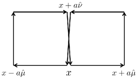
Figure 1: A $2\times 1$ twisted Wilson loop $T_{\mu\nu}(x)$.

We can check the naive continuum limit of this lattice action using the Baker-Campbell-Hausdorff (BCH) formula. The temporal plaquette may be evaluated as

$$P_{0i}(x)=\exp\Big{(}iabF_{0i}(x)+\mathcal{O}(a^{2}b,ab^{2})\Big{)}\,.$$ (5)

Hence

$$\begin{split}&\sum_{x}\sum_{i=1}^{D}\mathrm{Re}\operatorname{Tr}\big{\{}\mathbb{1}-P_{0i}(x)\big{\}}\\ &=\frac{a^{2}b^{2}}{2}\sum_{x}\sum_{i=1}^{D}\operatorname{Tr}\left\{F_{0i}(x)^{2}\right\}+\mathcal{O}(a^{3}b^{2},a^{2}b^{3}).\end{split}$$ (6)

Next, the twisted loop is given (cf. appendix A) by

$$T_{ij}(x)=\exp\big{(}ia^{3}D^{\mathrm{ad}}_{i}F_{ij}(x)+\mathcal{O}(a^{4})\big{)}\,.$$ (7)

Then

$$\quad\sum_{x}\sum_{j=1}^{D}\mathrm{Re}\operatorname{Tr}\bigg{\{}\mathbb{1}-\prod_{\begin{subarray}{c}i=1\\ i\neq j\end{subarray}}^{D}T_{ij}(x)\bigg{\}}$$

$$=\sum_{x}\sum_{j=1}^{D}\mathrm{Re}\operatorname{Tr}\bigg{\{}\mathbb{1}-\exp\bigg{(}ia^{3}\sum_{i=1}^{D}D^{\mathrm{ad}}_{i}F_{ij}(x)+\mathcal{O}(a^{4})\bigg{)}\bigg{\}}$$

$$=\frac{a^{6}}{2}\sum_{x}\sum_{j=1}^{D}\operatorname{Tr}\bigg{\{}\bigg{(}\sum_{i=1}^{D}D^{\mathrm{ad}}_{i}F_{ij}(x)\bigg{)}^{2}\bigg{\}}+\mathcal{O}(a^{7}).$$ (8)

Collecting Eqs. (6) and (8),

$$\begin{split}S_{\mathrm{lat}}&\to\frac{1}{2}\int\mathrm{d}x_{0}\mathrm{d}^{D}x\bigg{[}\frac{1}{e_{\mathrm{lat}}^{2}}\frac{b}{a^{D-2}}\sum_{i=1}^{D}\operatorname{Tr}\left\{F_{0i}(x)^{2}\right\}\\ &\quad+\frac{1}{g_{\mathrm{lat}}^{2}}\frac{a^{6-D}}{b}\sum_{j=1}^{D}\operatorname{Tr}\bigg{\{}\bigg{(}\sum_{i=1}^{D}D^{\mathrm{ad}}_{i}F_{ij}(x)\bigg{)}^{2}\bigg{\}}\bigg{]}\end{split}$$ (9)

as $a,b\to 0$. This reproduces the continuum action (1).

For completeness we outline the lattice discretization of other possible terms in the action in appendix B.

Matching with the continuum action (1) yields

$$\frac{1}{e^{2}}=\frac{1}{e_{\mathrm{lat}}^{2}}\frac{b}{a^{D-2}}\quad\text{and}\quad\frac{1}{g^{2}}=\frac{1}{g_{\mathrm{lat}}^{2}}\frac{a^{6-D}}{b}\,.$$ (10)

The two terms in Eq. (4) are of the same order only if we take the limit $a,b\to 0$ with $b/a^{2}\sim\mathcal{O}(1)$. Plugging this scaling into Eq. (10), we find $e_{\mathrm{lat}}^{2}\sim e^{2}a^{4-D}$ and $g_{\mathrm{lat}}^{2}\sim g^{2}a^{4-D}$. Now, let us consider the continuum limit in each dimension:

• $D=2$ ($d=2+1$): $e^{2}_{\mathrm{lat}}$, $g^{2}_{\mathrm{lat}}\propto a^{2}~{}\Rightarrow~{}$ $e_{\mathrm{lat}}$, $g_{\mathrm{lat}}\to 0$   with $e_{\mathrm{lat}}/g_{\mathrm{lat}}\sim\mathcal{O}(1)$.

• $D=3$ ($d=3+1$): $e^{2}_{\mathrm{lat}}$, $g^{2}_{\mathrm{lat}}\propto a^{1}~{}\Rightarrow~{}$ $e_{\mathrm{lat}}$, $g_{\mathrm{lat}}\to 0$   with $e_{\mathrm{lat}}/g_{\mathrm{lat}}\sim\mathcal{O}(1)$.

• $D=4$ ($d=4+1$): $e^{2}_{\mathrm{lat}}$, $g^{2}_{\mathrm{lat}}\propto a^{0}~{}\Rightarrow~{}$ It is unclear how to take the continuum limit at tree level.

This means that the continuum limit for $D=2$ and $3$ ($d=3$ and $4$) is reached trivially by sending $e_{\mathrm{lat}}$ and $g_{\mathrm{lat}}$ to $0$. However, $D=4$ ($d=5$) is the critical dimension where there is no scaling of the couplings at tree level. In $D=4$, the one-loop $\beta$ functions Horava (2010) are given by

$$\frac{\mathrm{d}}{\mathrm{d}\log\mu}e(\mu) =-\frac{3}{2}C_{2}e^{2}g+\cdots$$ (11a)

$$\frac{\mathrm{d}}{\mathrm{d}\log\mu}g(\mu) =-\frac{35}{6}C_{2}eg^{2}+\cdots,$$ (11b)

or, with $g_{\mathrm{YM}}\equiv\sqrt{eg}$ and $\lambda\equiv g/e$,

$$\frac{\mathrm{d}}{\mathrm{d}\log\mu}g_{\mathrm{YM}}(\mu) =-\frac{11}{3}C_{2}g^{3}_{\mathrm{YM}}+\mathcal{O}(g^{5}_{\mathrm{YM}})$$ (12a)

$$\frac{\mathrm{d}}{\mathrm{d}\log\mu}\lambda(\mu) =-\frac{13}{3}C_{2}g^{2}_{\mathrm{YM}}\lambda+\mathcal{O}(g^{4}_{\mathrm{YM}}\lambda)\,,$$ (12b)

where $C_{2}\equiv N/(4\pi^{2})$ for the gauge group $\text{SU}(N)$. The theory is asymptotically free and therefore the continuum limit is achieved by sending both $g_{\mathrm{YM}}$ and $\lambda$ to $0$. Solving Eqs. (12a) and (12b) simultaneously, we find

$$\lambda(\mu)\propto\big{(}g_{\mathrm{YM}}(\mu)\big{)}^{13/11}\,,~{}~{}~{}~{}\text{i.e.,}~{}~{}~{}g\propto e^{35/9}\,.$$ (13)

This scaling defines lines of constant physics in the weak-coupling region on the $(e,g)$ plane. The renormalization group flow of $e$ and $g$ is displayed in Fig. 2. (Since $C_{2}$ only enters the $\beta$ functions (11) as a multiplicative factor, the flow pattern is the same for all $N\geq 2$.) Integrating Eq. (12a), we encounter an infrared energy scale which survives the continuum limit:

$$\Lambda=\frac{1}{a}\exp\bigg{(}-\frac{24\pi^{2}}{11}\frac{1}{Ng^{2}_{\mathrm{YM}}(\frac{1}{a})}\bigg{)}\,.$$ (14)

This is the phenomenon called dimensional transmutation.

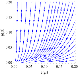
Figure 2: The flow diagram of $e$ and $g$ for the $\text{SU}(N)$ gauge group. The origin is a UV fixed point.

The above formulation is straightforwardly applicable to Abelian gauge theories as well. The geometrical structure of the lattice action is the same, with $\text{SU}(N)$ link variables replaced with $\text{U}(1)$ link variables. However, the resultant compact $\text{U}(1)$ gauge theory is not asymptotically free in $D=4$ $(d=5)$.

III Numerical simulation

We apply the above formulation to the lattice Monte Carlo simulation. The simulation can be done with standard algorithms in the lattice Yang-Mills theory. In this work, we performed a simulation of the lattice Hořava-Lifshitz theory for the case of $\text{SU}(N=3)$ gauge group.

First we examine the bulk phase structure on the $(e,g)$ plane. We calculated the action density $s\equiv\langle S_{\mathrm{lat}}\rangle/N_{\mathrm{lat}}$ for various values of the lattice couplings defined as

$$\beta_{e}\equiv\frac{2N}{e_{\mathrm{lat}}^{2}}~{}~{}~{}\text{and}~{}~{}~{}\beta_{g}\equiv\frac{2N}{g_{\mathrm{lat}}^{2}}\,.$$ (15)

The lattice size is $N_{\mathrm{lat}}=6^{5}$. (We partially checked the volume independence of the action density on a $10^{5}$ lattice.) For isotropic couplings ($\beta_{e}=\beta_{g}\equiv\beta$), we find using standard analytical methods Creutz (1983) that the action density behaves as

$$s =D\beta+\mathcal{O}(\beta^{2}) (\beta\to 0),$$ (16a)

$$s =(N^{2}-1)D/2+\mathcal{O}(1/\beta) (\beta\to\infty),$$ (16b)

respectively. This is useful in checking numerical data.

In Fig. 3, we show the simulation results for isotropic couplings $\beta\equiv\beta_{e}=\beta_{g}$. For comparison, we also show simulation results of the isotropic Yang-Mills theory in five dimensions. As already known, there is a jump at $\beta=4$–5 in the five-dimensional lattice Yang-Mills theory Itou et al. (2014). This jump indicates a bulk first-order phase transition from a confining phase to a deconfined phase. This bulk phase transition is a lattice artifact. Its existence reflects the non-renormalizable nature of the lattice Yang-Mills theory in five dimensions. On the other hand, there seems to be no phase transition in the Hořava-Lifshitz theory. In Fig. 3, the dashed lines are asymptotics in the strong coupling limit (16a) and in the weak coupling limit (16b) . The action density varies smoothly from the strong coupling limit to the weak coupling limit. As shown in Fig. 4, there is no discontinuity in the region $1\leq\beta_{e}\leq 9$ and $1\leq\beta_{g}\leq 9$. Thus, we can smoothly take the continuum limit of the lattice Hořava-Lifshitz theory.

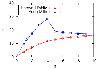
Figure 3: Action density with isotropic coupling constants $\beta\,(\,\equiv\beta_{e}=\beta_{g})$. The data of the Hořava-Lifshitz theory and the isotropic Yang-Mills theory on a $6^{5}$ lattice are plotted. The dashed lines are analytic results in the strong coupling limit ($\beta\to 0$) and the weak coupling limit ($\beta\to\infty$).

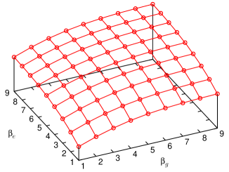
Figure 4: Action density of the Hořava-Lifshitz theory as a function of $\beta_{e}$ and $\beta_{g}$. The data on a $6^{5}$ lattice are plotted. Statistical error bars are omitted.

Next we study a rectangular Wilson loop $W_{0i}$ lying in the $(x_{0},x_{i})$ plane. The lattice size is $N_{\mathrm{lat}}=10^{5}$. The temporal Wilson loop may be interpreted as the infinite mass limit of a quark-antiquark system. (Although a Lifshitz-type fermion action admits various kinds of terms Anselmi (2009a, b); Dhar et al. (2009); Bakas (2012), this interpretation for the temporal Wilson loop should be correct provided that fermions couple to the temporal gauge field in a minimal way, as $\overline{\psi}\gamma_{0}D_{0}\psi$.) It gives the color singlet potential

$$V(x)=-\lim_{t\to\infty}\frac{1}{t}\ln\langle W_{0i}(t,x)\rangle.$$ (17)

In numerical simulations, the extrapolation to the limit $t\to\infty$ is done through a numerical fitting in a large but finite range of $t$. To check the fit-range independence, we plot the effective mass $bV_{\rm eff}(t,x)=-\langle\ln\{W_{0i}(t+b,x)/W_{0i}(t,x)\}\rangle$ in Fig. 5. The fit-range independence is clearly seen.

In Fig. 6 we show numerical results of the color singlet potential. The potential is linear. Therefore the Hořava-Lifshitz theory is a confining theory. We can analytically calculate the color singlet potential in two different limits: (i) In the strong coupling limit, the strong coupling expansion is justified. At leading order, we can prove that the Wilson loop obeys an area law and thus the potential is linear. The proof is exactly the same as the famous proof in the Yang-Mills theory Wilson (1974) because the temporal component of the lattice action is given by the plaquettes $P_{0i}$ both in the Hořava-Lifshitz theory and in the Yang-Mills theory. (ii) In the short distance limit, the perturbative loop expansion is justified because the theory is asymptotically free. Since the gluon propagator of $A_{0}$ is $\sim 1/p^{2}$, the perturbative one-gluon-exchange potential is $V(x)\sim\int\mathrm{d}^{D}p\exp(-ipx)/p^{2}\sim 1/x^{2}$. However, this correction cannot be seen in Fig. 6. Its coefficient must be very small or zero.

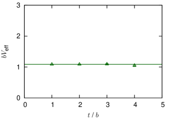
Figure 5: Effective mass $V_{\rm eff}(t,x)$ at $x/a=2$. The data from simulations on a $10^{5}$ lattice with $\beta\,(\,\equiv\beta_{e}=\beta_{g})=9$ are plotted.

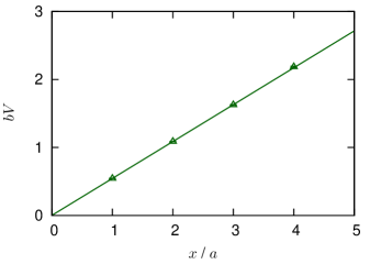
Figure 6: Color singlet potential $V(x)$. The data from simulations on a $10^{5}$ lattice with $\beta\,(\,\equiv\beta_{e}=\beta_{g})=9$ are plotted.

We also measured the expectation values of spatial plaquettes $P_{ij}$ and spatial Wilson loops $W_{ij}$ and found them to be zero within errors. This means in particular that the field strength $\operatorname{Tr}(F_{ij}^{2})$ is not induced in the action, which is consistent with the renormalizability of the theory due to the detailed balance condition Horava (2010). They can be nonzero if spatial plaquettes or other deformation terms are added to the action.

IV Summary

We proposed a lattice formulation of the Hořava-Lifshitz-type gauge theory. For a non-Abelian gauge group they are asymptotically free even in five dimensions. We performed the first Monte Carlo simulation of this theory on a lattice for the $\text{SU}(3)$ gauge group. Numerical results suggest that the continuum limit can be taken smoothly, in contrast to the ordinary Yang-Mills theory in five dimensions which is beset with a bulk phase transition. Using the present framework one can study various nonperturbative aspects of the Hořava-Lifshitz-type gauge theories by means of numerical lattice simulations. For example, it is straightforward to compactify a temporal or spatial direction and study possible center symmetry breaking. Of course one can perform simulations for other gauge groups and in other spacetime dimensions. Lattice simulations may also be performed with additional terms in the action, such as $\operatorname{Tr}(F_{ij}^{2})$, $\operatorname{Tr}(F_{ij}F_{jk}F_{ki})$, and $\operatorname{Tr}\big{\{}(D_{i}^{\mathrm{ad}}F_{jk})(D_{i}^{\mathrm{ad}}F_{jk})\big{\}}$, as discussed in appendix B. The interplay of these terms is an interesting subject. A more ambitious generalization is to include fermions coupled to the gauge field and study spontaneous chiral symmetry breaking. These issues are left for future works.

Appendix A Classical continuum limit

It has been known from (Luscher and Weisz, 1985, Eq. (16)) that a spatial plaquette in the naive continuum limit $a\to 0$ becomes

$$P_{ij}(x)\equiv U_{i}(x)U_{j}(x+a\hat{i})U_{i}(x+a\hat{j})^{\dagger}U_{j}(x)^{\dagger}$$

$$=\exp\Big{(}ia^{2}F_{ij}(x)+\frac{i}{2}a^{3}(D^{\mathrm{ad}}_{i}+D^{\mathrm{ad}}_{j})F_{ij}(x)+\mathcal{O}(a^{4})\Big{)}\,.$$ (18)

Because a twisted $2\times 1$ Wilson loop is a product of two neighboring spatial plaquettes, we get

$$\quad T_{ij}(x)$$

$$=\exp\Big{(}ia^{2}F_{ij}(x)+\frac{i}{2}a^{3}(D^{\mathrm{ad}}_{i}+D^{\mathrm{ad}}_{j})F_{ij}(x)+\mathcal{O}(a^{4})\Big{)}$$

$$~{}\times\exp\Big{(}\!-ia^{2}F_{ij}(x)-\frac{i}{2}a^{3}(-D^{\mathrm{ad}}_{i}+D^{\mathrm{ad}}_{j})F_{ij}(x)+\mathcal{O}(a^{4})\Big{)}$$

$$=\exp\big{(}ia^{3}D^{\mathrm{ad}}_{i}F_{ij}(x)+\mathcal{O}(a^{4})\big{)}\,,$$ (19)

which proves (7).

Appendix B More general lattice action

Besides $\operatorname{Tr}\{(D_{i}^{\mathrm{ad}}F_{ik})(D_{j}^{\mathrm{ad}}F_{jk})\}$, there are many other terms that could have been added to the action (1). In this appendix we discuss how to discretize them on a lattice.

Firstly, the term $\operatorname{Tr}\left({F_{ij}F_{jk}F_{ki}}\right)$ can be realized on a lattice as follows. Let us consider

$$\operatorname{Tr}\left\{\left({\mathbb{1}-P_{ij}(x)}\right)\left({\mathbb{1}-P_{jk}(x)}\right)\left({\mathbb{1}-P_{ki}(x)}\right)\right\}\,.$$ (20)

This expression is manifestly gauge invariant. By plugging in (18) for each $P$ and expanding in powers of $a$ we get

$$\eqref{eq:FFF} =ia^{6}\operatorname{Tr}\left\{F_{ij}(x)F_{jk}(x)F_{ki}(x)\right\}+\mathcal{O}(a^{7})\,,$$ (21)

which is the desired term.

The second term of our interest is $\operatorname{Tr}\left\{D_{k}^{\mathrm{ad}}F_{ij}(x)D_{k}^{\mathrm{ad}}F_{ij}(x)\right\}$. The case with $k=i$ or $k=j$ follows from $T_{ij}(x)$ as given in (7), so it is enough to assume here that $i,j$ and $k$ are distinct from each other, which requires $D\geq 3$.

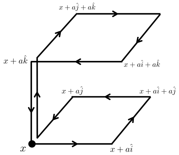
Figure 7: A Wilson loop on a lattice which reproduces $\operatorname{Tr}\{(D_{k}^{\mathrm{ad}}F_{ij})(D_{k}^{\mathrm{ad}}F_{ij})\}$ in the continuum limit.

Let us start from a Wilson loop $W_{ijk}(x)$ shown in Fig. 7:

$$W_{ijk}(x) \equiv P_{ij}(x)U_{k}(x)P_{ij}(x+a\hat{k})^{\dagger}U_{k}(x)^{\dagger}$$

$$=\operatorname{e}^{a^{2}\mathfrak{P}_{1}}\operatorname{e}^{iaA_{k}(x)+\mathcal{O}(a^{2})}\operatorname{e}^{-a^{2}\mathfrak{P}_{2}}\operatorname{e}^{-iaA_{k}(x)+\mathcal{O}(a^{2})}\,,$$

where from (18)

$$\mathfrak{P}_{1} \equiv iF_{ij}(x)+\frac{i}{2}a(D^{\mathrm{ad}}_{i}+D^{\mathrm{ad}}_{j})F_{ij}(x)+\mathcal{O}(a^{2})\,,$$

$$\mathfrak{P}_{2} \equiv iF_{ij}(x+a\hat{k})+\frac{i}{2}a(D^{\mathrm{ad}}_{i}+D^{\mathrm{ad}}_{j})F_{ij}(x+a\hat{k})+\mathcal{O}(a^{2})$$

$$=\mathfrak{P}_{1}+ia\partial_{k}F_{ij}(x)+\mathcal{O}(a^{2})\,.$$

Using the BCH formula,

$$W_{ijk}(x) =\exp\Big{(}a^{2}(\mathfrak{P}_{1}-\mathfrak{P}_{2})-ia^{3}[A_{k}(x),\mathfrak{P}_{2}]+\mathcal{O}(a^{4})\Big{)}$$

$$=\exp\big{(}\!-ia^{3}D_{k}^{\mathrm{ad}}F_{ij}(x)+\mathcal{O}(a^{4})\big{)}\,,$$ (22)

so that

$$\mathrm{Re}\operatorname{Tr}\{\mathbb{1}-W_{ijk}(x)\} =\frac{1}{2}a^{6}\operatorname{Tr}\left\{D_{k}^{\mathrm{ad}}F_{ij}(x)D_{k}^{\mathrm{ad}}F_{ij}(x)\right\}$$

$$\quad+\mathcal{O}(a^{7})\,.$$ (23)

However, it has been known from (Weisz, 1983, Eq. (2.10)) that $\operatorname{Tr}\left\{(D_{i}^{\mathrm{ad}}F_{ik})(D_{j}^{\mathrm{ad}}F_{jk})\right\}$, $\operatorname{Tr}\left\{F_{ij}(x)F_{jk}(x)F_{ki}(x)\right\}$ and $\operatorname{Tr}\left\{D_{k}^{\mathrm{ad}}F_{ij}(x)D_{k}^{\mathrm{ad}}F_{ij}(x)\right\}$ are linearly dependent, up to a total derivative. Thus it is sufficient to keep only two of them in the action.

The lattice actions for other possible terms like $\varepsilon_{jklm}\operatorname{Tr}\left\{D_{i}^{\mathrm{ad}}F_{jk}(x)D_{i}^{\mathrm{ad}}F_{lm}(x)\right\}$ (for $D=4$) can be worked out along similar lines.

References

- Lifshitz (1941a) E. M. Lifshitz, Zh. Eksp. Teor. Fiz. D 11, 255 (1941a).
- Lifshitz (1941b) E. M. Lifshitz, Zh. Eksp. Teor. Fiz. D 11, 269 (1941b).
- Horava (2009) P. Horava, Phys.Rev. D79, 084008 (2009), arXiv:0901.3775 [hep-th] .
- Anselmi (2009a) D. Anselmi, Annals Phys. 324, 874 (2009a), arXiv:0808.3470 [hep-th] .
- Anselmi (2009b) D. Anselmi, Annals Phys. 324, 1058 (2009b), arXiv:0808.3474 [hep-th] .
- Horava (2010) P. Horava, Phys.Lett. B694, 172 (2010), arXiv:0811.2217 [hep-th] .
- Visser (2009) M. Visser, Phys.Rev. D80, 025011 (2009), arXiv:0902.0590 [hep-th] .
- Dijkgraaf et al. (2010) R. Dijkgraaf, D. Orlando, and S. Reffert, Nucl.Phys. B824, 365 (2010), arXiv:0903.0732 [hep-th] .
- Anselmi (2010) D. Anselmi, Eur.Phys.J. C65, 523 (2010), arXiv:0904.1849 [hep-ph] .
- Chen and Huang (2010) B. Chen and Q.-G. Huang, Phys.Lett. B683, 108 (2010), arXiv:0904.4565 [hep-th] .
- Dhar et al. (2009) A. Dhar, G. Mandal, and S. R. Wadia, Phys.Rev. D80, 105018 (2009), arXiv:0905.2928 [hep-th] .
- Das and Murthy (2009) S. R. Das and G. Murthy, Phys.Rev. D80, 065006 (2009), arXiv:0906.3261 [hep-th] .
- Iengo et al. (2009) R. Iengo, J. G. Russo, and M. Serone, JHEP 0911, 020 (2009), arXiv:0906.3477 [hep-th] .
- Kawamura (2010) Y. Kawamura, Prog.Theor.Phys. 122, 831 (2010), arXiv:0906.3773 [hep-ph] .
- Orlando and Reffert (2010) D. Orlando and S. Reffert, Phys.Lett. B683, 62 (2010), arXiv:0908.4429 [hep-th] .
- Kaneta and Kawamura (2010) K. Kaneta and Y. Kawamura, Mod.Phys.Lett. A25, 1613 (2010), arXiv:0909.2920 [hep-ph] .
- Das and Murthy (2010) S. R. Das and G. Murthy, Phys.Rev.Lett. 104, 181601 (2010), arXiv:0909.3064 [hep-th] .
- Alexandre et al. (2010) J. Alexandre, K. Farakos, P. Pasipoularides, and A. Tsapalis, Phys.Rev. D81, 045002 (2010), arXiv:0909.3719 [hep-th] .
- Andreev (2010) O. Andreev, Int.J.Mod.Phys. A25, 2087 (2010), arXiv:0910.1613 [hep-th] .
- Chao (2009) W. Chao, (2009), arXiv:0911.4709 [hep-th] .
- Dhar et al. (2010) A. Dhar, G. Mandal, and P. Nag, Phys.Rev. D81, 085005 (2010), arXiv:0911.5316 [hep-th] .
- Iengo and Serone (2010) R. Iengo and M. Serone, Phys.Rev. D81, 125005 (2010), arXiv:1003.4430 [hep-th] .
- Romero et al. (2010) J. M. Romero, J. A. Santiago, O. Gonzalez-Gaxiola, and A. Zamora, Mod.Phys.Lett. A25, 3381 (2010), arXiv:1006.0956 [hep-th] .
- Anagnostopoulos et al. (2010) K. Anagnostopoulos, K. Farakos, P. Pasipoularides, and A. Tsapalis, (2010), arXiv:1007.0355 [hep-th] .
- Kobakhidze et al. (2011) A. Kobakhidze, J. E. Thompson, and R. R. Volkas, Phys.Rev. D83, 025007 (2011), arXiv:1010.1068 [hep-th] .
- Bakas and Lust (2011) I. Bakas and D. Lust, Fortsch.Phys. 59, 937 (2011), arXiv:1103.5693 [hep-th] .
- Hatanaka et al. (2011) H. Hatanaka, M. Sakamoto, and K. Takenaga, Phys.Rev. D84, 025018 (2011), arXiv:1105.3534 [hep-ph] .
- Eune et al. (2011) M. Eune, W. Kim, and E. J. Son, Phys.Lett. B703, 100 (2011), arXiv:1105.5194 [hep-th] .
- He et al. (2011) X.-G. He, S. S. Law, and R. R. Volkas, Phys.Rev. D84, 125017 (2011), arXiv:1107.3345 [hep-ph] .
- Gomes and Gomes (2012a) P. R. Gomes and M. Gomes, Phys.Rev. D85, 085018 (2012a), arXiv:1107.6040 [hep-th] .
- Farakos and Metaxas (2012a) K. Farakos and D. Metaxas, Phys.Lett. B707, 562 (2012a), arXiv:1109.0421 [hep-th] .
- Bakas (2012) I. Bakas, Fortsch.Phys. 60, 224 (2012), arXiv:1110.1332 [hep-th] .
- Kikuchi (2012) K. Kikuchi, Prog.Theor.Phys. 127, 409 (2012), arXiv:1111.6075 [hep-th] .
- Farias et al. (2012) C. Farias, M. Gomes, J. Nascimento, A. Y. Petrov, and A. da Silva, Phys.Rev. D85, 127701 (2012), arXiv:1112.2081 [hep-th] .
- Gomes and Gomes (2012b) P. R. Gomes and M. Gomes, Phys.Rev. D85, 065010 (2012b), arXiv:1112.3887 [hep-th] .
- Farakos and Metaxas (2012b) K. Farakos and D. Metaxas, Phys.Lett. B711, 76 (2012b), arXiv:1112.6080 [hep-th] .
- Farakos (2012) K. Farakos, Int.J.Mod.Phys. A27, 1250168 (2012), arXiv:1204.5622 [hep-th] .
- Montani and Schaposnik (2012) H. Montani and F. Schaposnik, Phys.Rev. D86, 065024 (2012), arXiv:1206.1027 [hep-th] .
- Farias et al. (2013) C. Farias, J. Nascimento, and A. Y. Petrov, Phys.Lett. B719, 196 (2013), arXiv:1208.3427 [hep-th] .
- Lozano et al. (2013) G. Lozano, F. A. Schaposnik, and G. Tallarita, Int.J.Mod.Phys. A28, 1350025 (2013), arXiv:1210.1182 [hep-th] .
- Adam et al. (2013) C. Adam, C. Naya, J. Sanchez-Guillen, and A. Wereszczynski, JHEP 1303, 012 (2013), arXiv:1212.2741 [hep-th] .
- Alves et al. (2013) V. S. Alves, B. Charneski, M. Gomes, L. Nascimento, and F. Pena, Phys.Rev. D88, 067703 (2013), arXiv:1303.6853 [hep-th] .
- Gomes et al. (2013) P. R. S. Gomes, P. Bienzobaz, and M. Gomes, Phys.Rev. D88, 025050 (2013), arXiv:1305.3792 [hep-th] .
- Alexandre and Brister (2013) J. Alexandre and J. Brister, Phys.Rev. D88, 065020 (2013), arXiv:1307.7613 [hep-th] .
- Hoyos et al. (2014) C. Hoyos, B. S. Kim, and Y. Oz, JHEP 1403, 029 (2014), arXiv:1309.6794 [hep-th] .
- Farias et al. (2014) C. Farias, M. Gomes, J. Nascimento, A. Y. Petrov, and A. da Silva, Phys.Rev. D89, 025014 (2014), arXiv:1311.6313 [hep-th] .
- Arav et al. (2014) I. Arav, S. Chapman, and Y. Oz, (2014), arXiv:1410.5831 [hep-th] .
- Alexandre (2011) J. Alexandre, Int.J.Mod.Phys. A26, 4523 (2011), arXiv:1109.5629 [hep-ph] .
- Hermele et al. (2004) M. Hermele, M. P. A. Fisher, and L. Balents, Phys. Rev. B 69,, 064404 (2004), cond-mat/0305401 .
- Moessner and Sondhi (2003) R. Moessner and S. L. Sondhi, Phys. Rev. B 68,, 184512 (2003), cond-mat/0307592 .
- Ardonne et al. (2004) E. Ardonne, P. Fendley, and E. Fradkin, Annals Phys. 310, 493 (2004), arXiv:cond-mat/0311466 [cond-mat] .
- Freedman et al. (2005) M. Freedman, C. Nayak, and K. Shtengel, Phys.Rev.Lett. 94, 147205 (2005), arXiv:cond-mat/0408257 [cond-mat] .
- Watanabe and Murayama (2014) H. Watanabe and H. Murayama, (2014), arXiv:1405.0997 [hep-th] .
- Banerjee et al. (2013) D. Banerjee, M. Bogli, M. Dalmonte, E. Rico, P. Stebler, et al., Phys.Rev.Lett. 110, 125303 (2013), arXiv:1211.2242 [cond-mat.quant-gas] .
- Tagliacozzo et al. (2013) L. Tagliacozzo, A. Celi, P. Orland, M. W. Mitchell, and M. Lewenstein, Nature Communications 4, 2615 (2013), arXiv:1211.2704 [cond-mat.quant-gas] .
- Zohar et al. (2013) E. Zohar, J. I. Cirac, and B. Reznik, Phys.Rev.Lett. 110, 125304 (2013), arXiv:1211.2241 [quant-ph] .
- Parisi and Wu (1981) G. Parisi and Y.-s. Wu, Sci.Sin. 24, 483 (1981).
- Zinn-Justin (1986) J. Zinn-Justin, Nucl.Phys. B275, 135 (1986).
- Bern et al. (1987) Z. Bern, M. Halpern, and L. Sadun, Nucl.Phys. B284, 92 (1987).
- Okano (1987) K. Okano, Nucl.Phys. B289, 109 (1987).
- Creutz (1979) M. Creutz, Phys.Rev.Lett. 43, 553 (1979).
- Dimopoulos et al. (2006) P. Dimopoulos, K. Farakos, and S. Vrentzos, Phys.Rev. D74, 094506 (2006), arXiv:hep-lat/0607033 [hep-lat] .
- Irges and Knechtli (2007) N. Irges and F. Knechtli, Nucl.Phys. B775, 283 (2007), arXiv:hep-lat/0609045 [hep-lat] .
- Irges and Knechtli (2010) N. Irges and F. Knechtli, Phys.Lett. B685, 86 (2010), arXiv:0910.5427 [hep-lat] .
- de Forcrand et al. (2010) P. de Forcrand, A. Kurkela, and M. Panero, JHEP 1006, 050 (2010), arXiv:1003.4643 [hep-lat] .
- Farakos and Vrentzos (2012) K. Farakos and S. Vrentzos, Nucl.Phys. B862, 633 (2012), arXiv:1007.4442 [hep-lat] .
- Knechtli et al. (2012) F. Knechtli, M. Luz, and A. Rago, Nucl.Phys. B856, 74 (2012), arXiv:1110.4210 [hep-lat] .
- Del Debbio et al. (2012) L. Del Debbio, A. Hart, and E. Rinaldi, JHEP 1207, 178 (2012), arXiv:1203.2116 [hep-lat] .
- Del Debbio et al. (2013) L. Del Debbio, R. D. Kenway, E. Lambrou, and E. Rinaldi, Phys.Lett. B724, 133 (2013), arXiv:1305.0752 [hep-lat] .
- Itou et al. (2014) E. Itou, K. Kashiwa, and N. Nakamoto, (2014), arXiv:1403.6277 [hep-lat] .
- Luscher and Weisz (1985) M. Luscher and P. Weisz, Commun.Math.Phys. 97, 59 (1985).
- Creutz (1983) M. Creutz, QUARKS, GLUONS AND LATTICES (Cambridge University Press, Cambridge, 1983).
- Note (1) In the strong coupling limit of the isotropic Yang-Mills theory in dimensions, . In the present case (), . In the weak coupling limit, the behavior of at leading order is the same as in the Hořava-Lifshitz theory and is given by (16b\@@italiccorr).
- Wilson (1974) K. G. Wilson, Phys.Rev. D10, 2445 (1974).
- Weisz (1983) P. Weisz, Nucl.Phys. B212, 1 (1983).