Joint cross-domain classification and subspace learning for unsupervised adaptation
Abstract
Domain adaptation aims at adapting the knowledge acquired on a source domain to a new different but related target domain. Several approaches have been proposed for classification tasks in the unsupervised scenario, where no labeled target data are available. Most of the attention has been dedicated to searching a new domain-invariant representation, leaving the definition of the prediction function to a second stage. Here we propose to learn both jointly. Specifically we learn the source subspace that best matches the target subspace while at the same time minimizing a regularized misclassification loss. We provide an alternating optimization technique based on stochastic sub-gradient descent to solve the learning problem and we demonstrate its performance on several domain adaptation tasks.
1 Introduction
In real world applications, having a probability distribution mismatch between the training and the test data is more often the rule than an exception. Think about part of speech tagging across different text corpora [5], localization over time with wifi signal distributions that get easily outdated [42], or biological models to be used across different subjects [38]. Computer vision methods are also particularly challenged in this respect: real world conditions may alter the image statistics in many complex ways (lighting, pose, background, motion blur etc.), to not even mention the difference in quality of the acquisition device (e.g. resolution), or the high number of possible artificial modifications obtained by post-processing (e.g. filtering). Due to this large variability, any learning algorithm trained on a source set regardless of the final target data will most likely produce poor, unsatisfactory results.
Domain adaptation techniques propose to overcome these issues and make use of information coming from both source and target domains during the learning process. In the unsupervised case, where no labeled samples are provided for the target, the most extensively studied paradigm consists in assuming the existence of a domain-invariant feature space and searching for it. In general all the techniques based on this idea focus on transforming the representation of the source and target samples to maximize some notion of similarity between them [14, 15, 12]. However in this way the classification task is left aside and the prediction model is learned only in a second stage. As thoroughly discussed in [2, 29], the choice of the feature representation able to reduce the domain divergence is indeed a crucial factor for the adaptation. Nevertheless it is not the only one. If several representations induce similar marginal distributions for the two domains, would a classifier perform equally well in all of them? Is it enough to encode the labeling information in the used feature space or is it better to learn a cross-domain classification model together with the optimal domain-invariant representation? Here we answer these questions by focusing on unsupervised domain adaptation subspace solutions. We present an algorithm that learns jointly both a low dimensional representation and a reliable classifier by optimizing a trade-off between the source-target similarity and the source training error.
2 Related Work
For classification tasks, the goal of domain adaptation is to learn a function from the source domain that predicts the class label of a novel test sample from the target domain [33]. In the literature there are two main scenarios depending on the availability of data annotations: the semi-supervised and the unsupervised setting.
In the semi-supervised setting a few labeled samples are provided for the target domain besides a large amount of annotated source data. Existing solutions can be divided into classifier-based and representation-based methods. The former modify the original formulation of Support Vector Machines (SVM) [41, 10] and other statistical classifiers [6]: they adapt a pre-trained model to the target, or learn the source and target classifiers simultaneously. The latter exploit the correspondence between source and target labeled data to impose constraints over the samples through metric learning [25, 34], or consider feature augmentation strategies [23] and manifold alignment [40]. Some approaches have also tackled the cases with more than two available domains [9, 19] and the unlabeled part of the target has been used for co-regularization [26]. Recently, two methods proposed to combine classifier-based and representation-based solutions. [20] introduced an approach to learn jointly a cross-domain classifier and a transformation that maps the target points into the source domain. Several kernel maps are used to encode the representation in [8], which proposed a domain transfer multiple kernel learning algorithm.
In the more challenging unsupervised setting, all the available target samples are unlabeled. Many unsupervised domain adaptive approaches resort to estimating the data distributions and minimizing a distance measure between them, while re-weighting/selecting the samples [38, 13]. The Maximum Mean Discrepancy (MMD) [16] maps two sets of data to a reproducing Kernel Hilbert Space and it has been largely used as distance measure between two domain distributions. Although endowed with nice properties, the choice of the kernel and kernel parameters are critical and, if non-optimal, can lead to a very poor estimate of the distribution distance [17]. Dictionary learning methods have also been used with the goal of defining new representations that overcome the domain shift [30, 35]. A reconstruction approach was proposed in [24]: the source samples are mapped into an intermediate space where each of them can be represented as a linear combination of the target domain samples.
Another promising direction for unsupervised domain adaptation is that of subspace modeling. This is based on the idea that source and target share a latent subspace where the domain shift is removed or reduced. As for dictionary learning, the approaches presented in this framework are mostly linear, but can be easily extended to non-linear spaces through explicit feature mappings [39]. In [4] Canonical Correlation Analysis (CCA) has been applied to find a coupled domain-invariant subspace. Principal Component Analysis (PCA) and other eigenvalue methods are also widely used for subspace generation. For instance, Transfer Component Analysis (TCA, [32]) is a dimensionality reduction approach that searches a latent space where the variance of the data is preserved as much as possible and the distance between the distributions is reduced. Transfer Subspace Learning (TSL, [37]) couples PCA and other subspace learning methods with a Bregman divergence-based regularization which measures the distance between the distribution in the projected space. Alternatively, the algorithm introduced in [1] uses MMD in the subspace to search for a domain invariant projection matrix. Other methods exploited multiple intermediate subspaces to link the source and the target data. This idea was introduced in [15] where the path across the domains is defined as a geodesic curve over a Grassmann manifold. This strategy has been further extended in [14] where all the intermediate subspaces are integrated to define a cross-domain similarity measure. Despite the intuitive characterization of the problem, it is not clear why all the subspaces along this path should yield meaningful representations. Recently the Subspace Alignment (SA) method [12] demonstrated that it is possible to map directly the source to the target subspace without necessarily passing through intermediate steps.
Overall, the main focus of the unsupervised methods proposed in the literature is on the domain invariance of the final data representation and less attention has been dedicated to its discriminative power. First attempts in this direction have been done in [14] by substituting the use of PCA over the source subspace with Partial Least Squares (PLS), and in [32] where SSTCA chooses the representation by maximizing its dependence on the data labels. Our work fits in this context. We aim at extending the integration of classifier-based with representation-based solutions in the unsupervised setting where no access to the target labels is available, not even for hyperparameter cross validation. Differently from all the described unsupervised approaches we go beyond searching only a domain invariant feature space and we want to optimize also a cross-domain classification model. We propose an algorithm that combines effectively subspace and max-margin learning and exploits the source discriminative information better than just encoding it in the representation. Our approach does not need an estimate of the source and target data distributions and relies on a simple measure of domain shift. Finally, in previous work the performance of the adaptive methods have been often evaluated by tuning the model parameters on the target data [12, 24] or by fixing them to default values [21]. Here we choose a more fair setup for unsupervised domain adaptation and we show that our approach outperforms different existing subspace adaptive methods by exploiting exclusively the source annotations. We name our algorithm Joint cross-domain Classification and Subspace Learning (JCSL).
In the following sections we define the notation that will be used in the rest of the paper (section 3) and we briefly review the theory of learning from different domains together with the subspace domain shift measure used in [12] from which we took inspiration. We then introduce our approach (section 4) followed by an extensive experimental analysis that shows its effectiveness on several domain adaptation tasks (section 5). We conclude with a final discussion and sketching possible directions for future research (section 6).
3 Problem Setup and Background
Let us consider a classification problem where the data instances are in the form . Here is the feature vector for the -th sample and is the corresponding label. We assume that labeled training samples are drawn from a source distribution , while a set of unlabeled test samples come from a different target distribution , such that it holds . In particular, the source and the target distributions satisfy the covariate shift property [36] if they have the same labeling function with , while the marginal distributions differ . We operate under this hypothesis.
A bound on the target domain error
Theoretical studies on domain adaptation have established the conditions under which a classifier trained on the source data can be expected to perform well on the target data. The following generalization bound on the target error has been demonstrated in [2]:
| (1) |
Here indicates the predictor function, while is the hypothesis class from which the predictor has been chosen. In words, the bound states that a low target error can be guaranteed if the source error , a measure of the domain distribution divergence , and the error of the ideal joint hypothesis on the two domains are small. The joint error can be written as where . The value of is supposed to be low under the the covariate shift assumption.
A subspace measure of domain shift
The low-dimensional intrinsic structure of the source and target domains can be specified by their corresponding orthonormal basis sets, indicated respectively as and . These are two full rank matrices, and is the subspace dimensionality. In [12], a transformation matrix is introduced to modify the source subspace. The domain shift of the transformed source basis with respect to the target is simply measured by the following function:
| (2) |
where is the Frobenius norm. The Subspace Alignment (SA) method proposed to minimize this measure, obtaining the optimal transformation matrix in closed form: . The matrix is finally used to represent the source data. The original domain basis sets can be obtained through different strategies, both unsupervised (PCA) and supervised (PLS, LDA), as extensively studied in [11].
SA has shown promising results for visual cross-domain classification tasks outperforming other subspace adaptive methods. However, on par with its competitors [15, 14], it keeps the domain adaptive process (learning M) and the classification process (e.g. learning an SVM model) separated, focusing only on the distribution divergence term of the bound in (1).
4 Proposed Approach
With the aim of minimizing both the domain divergence and the source error in (1), we propose an algorithm that learns a domain-invariant representation and an optimal cross-domain classification model. For the representation we concentrate on subspace methods and we take inspiration from the SA approach. For the classification we rely on a standard max-margin formulation. The details of our Joint cross-domain Classification and Subspace Learning (JCSL) algorithm are described below.
Given a fixed target subspace basis we minimize the following regularized risk functional
| (3) |
Here the regularization terms aim at optimizing separately the linear source classification model , and the source representation matrix , while the loss function depends on their combination. For our analysis we choose the hinge loss: , but other loss functions can be used for different cross-domain applications. The parameters and allows to define a trade-off between the importance of the terms in the objective function. In particular a high value pushes towards giving more importance to the distribution divergence term, while a high value focuses the attention on the training error term to improve the classification performance in the new space.
The matrix has a role analogous to that of in SA, however in our case it is not necessary to specify a priori the source subspace which is now optimized together with the alignment transformation matrix in a single step. Note that, if the source and target data can be considered as belonging to the same domain (no domain shift), our method will automatically provide boiling down to standard learning in the shared subspace. We follow previous literature and propose the use of PCA to define the target subspace [12, 14]. Besides having demonstrated good results empirically, the theoretical meaning of this choice can be identified by writing the mutual information between the target and the source as
| (4) |
Projecting the target data to the subspace maximizes the entropy , while our objective function minimizes the domain shift, which is related to the Kullback-Leibler divergence . Hence, we expect to increase the mutual information between source and target.
Minimizing (3) jointly over is a non-convex problem and finding a global optimum is generally intractable. However we can apply alternated minimization for and resulting in two interconnected convex problems that can be efficiently solved by stochastic subgradient descent. For this procedure we need the partial derivatives of (3) that can be easily calculated as:
| (5) |
where and are the derivatives of with respect to and . When using the hinge loss we get
The iterative subgradient descent procedure terminates when the algorithm converges, showing a negligible change of either or between two consecutive iterations. The formulation holds for a binary classifier but can easily be used in its one-vs-all multiclass extension that highly benefits from the choice of the stochastic variant of the optimization process.
At test time, we indicate the classification score of class for the target sample as . The multiclass final prediction is then obtained by maximizing over the scores: . Note that the source representation matrix is not involved at this stage, and the target subspace basis appears instead. Differently from the pre-existing unsupervised domain adaptation methods that encode the discriminative information in the representation, JCSL learns directly a domain invariant classification model able to generalize from source to target. The JCSL learning strategy is summarized in Algorithm 1.
5 Experiments
We validate our approach over several domain adaptation tasks. In the following we first describe our experimental setting (section 5.1) and then we report on the obtained results (sections 5.2, 5.3, 5.4). Moreover we present a detailed analysis on the role of the learning parameters and on the domain-shift reduction effect of JCSL (section 5.2).
 |
 |
| DA Problem | NA | SA(LDA-PCA) | GFK(LDA-PCA) | TCA | SSTCA | TSL | JCSL | |
| AC | 38.1 2.6 | 41.11.7 | 43.4 3.2 | 43.2 3.7 | 43.5 3.2 | 38.82.4 | 40.40.9 | 42.6 0.9 |
| AD | 32.9 2.8 | 37.51.4 | 44.7 2.6 | 43.7 2.8 | 38.8 2.1 | 34.16.9 | 40.81.7 | 42.5 3.2 |
| AW | 36.8 2.9 | 39.12.8 | 40.3 2.9 | 41.3 2.0 | 41.0 1.0 | 34.13.8 | 41.12.3 | 47.6 2.1 |
| CA | 39.5 1.0 | 40.62.8 | 39.3 1.8 | 39.9 1.5 | 42.5 1.2 | 39.13.5 | 43.04.2 | 44.3 1.2 |
| CD | 38.8 2.4 | 40.91.3 | 44.0 2.0 | 42.0 2.5 | 42.1 2.5 | 38.34.1 | 40.43.4 | 46.5 1.5 |
| CW | 37.8 1.4 | 35.93.2 | 37.3 3.3 | 41.8 3.8 | 39.4 2.5 | 31.64.9 | 40.92.4 | 46.5 2.0 |
| DA | 24.4 1.7 | 30.62.7 | 35.7 2.3 | 31.0 2.7 | 30.4 2.1 | 38.02.6 | 39.61.2 | 41.3 0.9 |
| DC | 30.5 2.1 | 37.91.3 | 41.5 1.4 | 40.9 2.8 | 36.7 2.6 | 32.91.8 | 33.42.1 | 35.1 0.9 |
| DW | 60.9 3.1 | 67.92.8 | 58.6 2.1 | 60.5 3.8 | 64.5 3.2 | 76.23.0 | 73.71.5 | 74.2 3.6 |
| WA | 29.7 1.7 | 34.11.7 | 34.7 0.9 | 33.1 1.2 | 34.6 1.4 | 35.12.6 | 38.01.6 | 43.1 1.0 |
| WC | 34.1 1.6 | 38.11.3 | 36.7 1.2 | 37.7 1.8 | 39.6 2.2 | 29.72.5 | 30.41.3 | 36.1 2.0 |
| WD | 71.1 2.6 | 74.60.9 | 69.5 2.4 | 75.3 2.6 | 77.3 2.7 | 69.93.4 | 66.91.6 | 66.2 2.9 |
| AVG. | 39.6 | 43.2 | 43.8 | 44.2 | 44.2 | 41.4 | 44.0 | 47.2 |
| MNISTUSPS | 45.4 | 45.1 | 48.6 | 34.6 | 40.8 | 40.6 | 43.5 | 46.7 |
| USPSMNIST | 33.3 | 33.4 | 22.2 | 22.6 | 27.4 | 22.2 | 34.1 | 35.5 |
| AVG. | 39.4 | 39.2 | 35.4 | 28.6 | 34.1 | 31.4 | 38.8 | 41.1 |
5.1 Datasets, baselines and implementation details
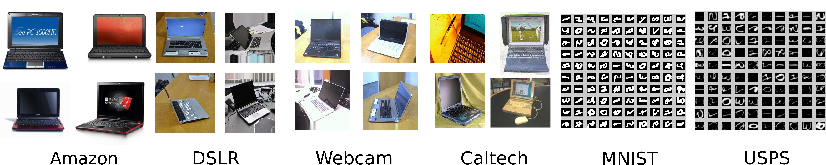
We choose three image datasets (see Figure 1) and a wifi signal dataset.
Office + Caltech [14]. This dataset was created by combining the Office dataset [34] with Caltech256 [18] and it contains images of 10 object classes over four domains: Amazon, Dslr, Webcam and Caltech. Amazon consists of images from online merchants’ catalogues, while Dslr and Webcam domains are composed by respectively high and low resolution images. Finally, Caltech corresponds to a subset of the original Caltech256. We use the features provided by Gong et al. [14]: SURF descriptors quantized into histograms of 800 bag-of-visual words and standardized by z-score normalization. All the 12 possible source-target domain pairs are considered. We use the data splits provided by Hoffman et al. [20].
MNIST [27] + USPS [22]. This dataset combines two existing image collections of digits presenting different gray scale data distributions. Specifically they share 10 classes of digits. We randomly selected 1800 images from USPS and 2000 images from MNIST. By following [28] we uniformly re-scale all images to size 16 16 and we use the L2-normalized gray-scale pixel values as feature vectors. Both domains are alternatively used as source and target.
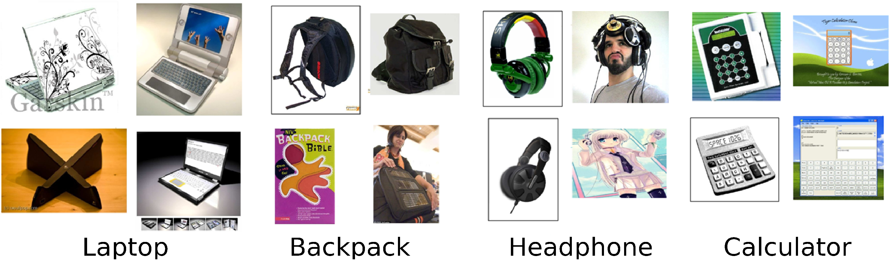
Bing+Caltech [3]. In this dataset, weakly annotated images from the Bing search engine define the source domain while images of Caltech256 are used as target. We run experiments varying the number of categories (5, 10, 15, 20, 25 and 30) and the number of source examples per category (5 and 10) using the same train/test split adopted in [3]. As typically done for this dataset, Classemes features are used as image representation [3].
WiFi [42]. This dataset was used in the 2007 IEEE ICDM contest for domain adaptation. The goal is to estimate the location of mobile devices based on the received signal strength (RSS) values from different access points. The domains correspond to two different time periods during which the collected RSS values present different distributions. The dataset contains 621 labeled examples collected during time period A (source) and 3128 unlabeled examples collected during time period B (target). The location recognition performance is generally evaluated by measuring the average error distance between the predicted and the correct space position of the mobile devices. We slightly modify the task to define a classification rather than a regression problem. We consider 247 locations and we evaluate the classification performance between the sets A and B with and without domain adaptation. We repeat the experiments both testing over all the target data and considering 10 random target splits, each with 400 random samples.
We benchmark JCSL 111We implemented our algorithm in MATLAB. The code is submitted with the paper as supplementary material. against the following subspace-based domain adaptation methods:
TCA, SSTCA: Transfer Component Analysis and its semi-supervised extension [32]. We implemented TCA and SSTCA by following the original paper description. For SSTCA we turned off the locality preserving option to have a fair comparison with all the other considered methods, none of which exploits local geometry222Following the original paper notation we fixed , , ..
TSL: Transfer Subspace Learning [37]. We used the code made publicly available by the authors333http://www.cs.utexas.edu/~ssi/TrFLDA.tar.gz which implements TLS by adding a Bregman-divergence based regularization to the Fisher’s Linear Discriminant Analysis (FLDA).
GFK(LDA-PCA), SA(LDA-PCA): for both the Geodesic Flow Kernel [14] and the Subspace Alignment [12] methods we slightly modified the original implementation provided by the authors444 http://www-scf.usc.edu/~boqinggo/domain_adaptation/GFK_v1.zip, http://homes.esat.kuleuven.be/~bfernand/DA_SA/downloadit.php?fn=DA_SA.zip to integrate the available discrimintive information in the source domain. As preliminary evaluation we compared the results of GFK and SA when the basis of the source subspace were obtained with PLS and LDA. Although performing similarly on average, PLS showed less stability than LDA with large changes in the outcome for small variations of the subspace dimensionality . This can be explained by considering the difficulty of finding the best that jointly maximizes the source data/label coherence and minimizes the source/target shift. Thus, for our experiments we rely on the more stable LDA for the source which fixes equal . On the other hand, the target subspace is always obtained by applying PCA and selecting the first eigenvectors.
As further baselines we also consider the source classifier learned with no adaptation (NA) in the original feature space and in the target subspace. The last one is obtained by applying PCA on the target domain and using the eigenvectors as basis to represent both the source and the target data ().
For all the methods the final classifier is a linear SVM with the parameter tuned by two-fold cross-validation on the source over the range . Our JCSL has three main parameters that are also chosen by two-fold cross validation on the source. We remark that the target data are not annotated, thus tuning the parameters on the source is the only feasible option. We searched for in the same range indicated before for . The parameter was tuned in both for JCSL and for the baselines , TSL, TCA and SSTCA.
We implemented the stochastic sub-gradient descent using a step size of and a batch size of . The alternating optimization converges for less than 100 iterations and we can obtain the results for any of the source-target domain pairs of the Office+Caltech (excluding feature extraction) in 2 minutes using a modern desktop computer (2.8GHz cpu, 4Gb of ram, 1 core). With respect to the considered competing methods, the training phase of JCSL is slower (e.g. 60 times slower with respect to SA and GFK), but we remark that JCSL provides an optimized cross-domain classifier besides reducing the data distribution shift. The test phase runtime is comparable for all the considered approaches. In practical applications domain adaptation models are usually learned offline, thus the training time is a minor issue.
 |
 |
5.2 Results - Office+Caltech and MNIST+USPS
The obtained results over the Office+Caltech and MNIST+USPS datasets are presented in Table 1. Overall JCSL outperforms the considered baselines in 7 source-target pairs out of 14 and shows the best average results over the two datasets. Thus, we can state that, minimizing a trade-off between source-target similarity and the source classification error pays off compared to only reducing the cross-domain representation divergence. Still SA shows an advantage with respect to JCSL in a few of the considered cases most probably because it can exploit the discriminative LDA subspace. With respect to JCSL , TCA and SSTCA seem to work particularly well when the domain shift is small (e.g. Amazon Caltech, Dslr Webcam). Interestingly JCSL is the only method that consistently outperforms NA over MNIST+USPS.
Parameter analysis
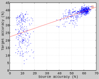
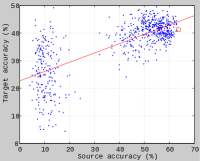
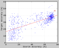
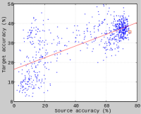
To better understand the performance of JCSL we analyze how the target accuracy varies with respect to the source accuracy while changing the learning parameters , and . The plots in Figure 2 consider four domain adaptation problems, namely (Amazon Caltech), (Amazon Webcam), (MNIST USPS) and (USPS MNIST)555Analogous results are obtained for all the remaining source-target pairs.. All of them present two main clusters. On the left, when the source accuracy is low, the target accuracy is uniformly distributed. This behavior mostly appears when is very small and has a high value: this indicates that minimizing only does not guarantee stable results on the target task. On the other hand, in the second cluster the source accuracy is highly correlated with the target accuracy. On average, for the points in this region, both the domain divergence term and the misclassification loss obtain low values. The final JCSL result with the optimal appears always in this area and the dimensionality of the subspace seems to have only a moderate influence on the final results. The red line reported on the plots is obtained by least-square fitting over the source and target accuracies and presents an analogous trend for all the considered source-target pairs. This is an indication that when domains are adaptable (negligible in (1)) our method is able to find a good source representation as well as a classifier that generalizes to the target domain.
Measuring the domain shift
For the same domain pairs considered above we also evaluate empirically the divergence measure defined in [2]. This is obtained by learning a linear SVM that discriminates between the source and target instances, respectively pseudo-labeled with and . We separated each domain into two halves and use them for training and test when learning a linear SVM model. A high final accuracy indicates high domain divergence. We perform this analysis by comparing the domain shift before and after the application of SA and JCSL, according to their standard settings. SA presents a single step and learns one subspace representation . JCSL exploits a one-vs-all procedure learning as many as the number of classes: each step involves all the data (no per class sample selection). The final domain shift for JCSL is the average over the obtained separate shift values. The results in Table 2 indicate that SA and JCSL produce comparable results in terms of domain-shift reduction, suggesting that the main advantage of JCSL comes from the learned classifier.
| Space | AC | AW | MNISTUSPS | USPSMNIST |
| Original features | 74.82 | 90.18 | 100.00 | 100.00 |
| SA | 65.96 | 56.56 | 55.78 | 55.74 |
| JCSL | 65.76 | 54.97 | 57.03 | 53.28 |
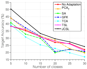
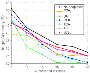
5.3 Results - Bing+Caltech
Due to the way in which it was defined, Bing+Caltech can be considered as a much more challenging testbed for unsupervised domain adaptation compared to the other used datasets (see also Figure 1). At the same time it also corresponds to one of the most realistic scenarios where domain adaptation is needed: we have access to only a limited number of noisy labeled source images obtained from the web and we want to use them to classify over a curated collection of object images. For this problem exploiting at the best all the available information is crucial. Specifically, since the source is not fully reliable, coding its discriminative information in the representation (e.g. through LDA or PLS) may be misleading. On the other hand, using the subspace of the non-noisy target data to guide the learning process can be much more beneficial.
As shown in Figure 3, JCSL is the only method that consistently improves over the non-adaptive approach independently from the number of considered classes. TSL is always equivalent to NA, while the other subspace methods, although initially helpful for problems with few classes, lose their advantage over NA when the number of classes increases. This behavior is almost equivalent when using both 5 and 10 source samples per class.
5.4 Results - WiFi Localization
To demonstrate the generality of the proposed algorithm, we evaluate JCSL also on non-visual data. Since the WiFi vector dimensionality (100) is lower than the number of classes (247), we do not exploit LDA here but we simply apply PCA to define the subspace dimensionality for both the source and target domains. The results on the WiFi-localization task are reported in Table 3 and show that domain adaptation is clearly beneficial.
| NA | SA | GFK | TCA | SSTCA | JCSL | |
| full | 16.6 | 17.3 | 17.3 | 19.0 | 18.5 | 20.2 |
| splits | 16.9 2.1 | 17.6 2.2 | 17.4 2.1 | 19.2 2.1 | 18.0 2.2 | 20.5 2.4 |
TCA and SSTCA are the state of the art linear methods on the WiFi dataset and they confirm their value even in the considered classification setting by outperforming SA and GFK. Still JCSL presents the best results. The obtained classification accuracy confirms the value of our method over the other subspace-based techniques.
6 Conclusions
Motivated by the theoretical results of Ben-David et al. [2], in this paper we proposed to integrate the learning process of the source prediction function with the optimization of the invariant subspace for unsupervised domain adaptation. Specifically, JCSL learns a representation that minimizes the divergence between the source subspace and the target subspace, while optimizing the classification model. Extensive experimental results have shown that, by taking advantage of the described principled combination and without the need of passing through the evaluation of the data distributions, JCSL outperform other subspace domain adaptation methods that focus only on the representation part.
Recently several works have demonstrated that Convolutional Neural Network classifiers are robust to domain shift [7, 31]. Reasoning at high level we can identify the cause of such a robustness on the same idea at the basis of JCSL : deep architectures learn jointly a discriminative representation and the prediction function. The highly non-linear transformation of the original data coded into the CNN activation values can also be used as input data descriptors for JCSL with the aim of obtaining a combined effect. As future work we plan to evaluate principled ways to find automatically the best subspace dimensionality using low-rank optimization methods.
Acknowledgments
The authors acknowledge the support of the FP7 EC project AXES and of the FP7 ERC Starting Grant 240530 COGNIMUND.
References
- [1] Mahsa Baktashmotlagh, Mehrtash Harandi, Brian Lovell, and Mathieu Salzmann. Unsupervised domain adaptation by domain invariant projection. In International Conference on Computer Vision (ICCV), 2013.
- [2] Shai Ben-David, John Blitzer, Koby Crammer, and Fernando Pereira. Analysis of representations for domain adaptation. In Neural Information Processing Systems (NIPS), 2007.
- [3] Alessandro Bergamo and Lorenzo Torresani. Exploiting weakly-labeled web images to improve object classification: a domain adaptation approach. In Neural Information Processing Systems (NIPS), 2010.
- [4] John Blitzer, Dean Foster, and Sham Kakade. Domain adaptation with coupled subspaces. In International Conference on Artificial Intelligence and Statistics (AISTATS), 2011.
- [5] John Blitzer, Ryan McDonald, and Fernando Pereira. Domain adaptation with structural correspondence learning. In Empirical Methods in Natural Language Processing (EMNLP), 2006.
- [6] Hal Daumé, III and Daniel Marcu. Domain adaptation for statistical classifiers. J. Artif. Int. Res., 26(1):101–126, May 2006.
- [7] Jeff Donahue, Yangqing Jia, Oriol Vinyals, Judy Hoffman, Ning Zhang, Eric Tzeng, and Trevor Darrell. Decaf: A deep convolutional activation feature for generic visual recognition. In International Conference in Machine Learning (ICML), 2014.
- [8] Lixin Duan, Ivor W. Tsang, and Dong Xu. Domain transfer multiple kernel learning. IEEE Transactions on Pattern Analysis and Machine Intelligence (PAMI), 34(3):465–479, March 2012.
- [9] Lixin Duan, Ivor W. Tsang, Dong Xu, and Tat-Seng Chua. Domain adaptation from multiple sources via auxiliary classifiers. In International Conference in Machine Learning (ICML), 2009.
- [10] Lixin Duan, Ivor W. Tsang, Dong Xu, and Stephen J. Maybank. Domain transfer svm for video concept detection. In Computer Vision and Pattern Recognition (CVPR), 2009.
- [11] Basura Fernando, Amaury Habrard, Marc Sebban, and Tinne Tuytelaars. Subspace alignment for domain adaptation. CoRR, abs/1409.5241, 2014.
- [12] Basura Fernando, Amaury Habrard, Marc Sebban, Tinne Tuytelaars, et al. Unsupervised visual domain adaptation using subspace alignment. In International Conference on Computer Vision (ICCV), 2013.
- [13] B. Gong, K. Grauman, and F. Sha. Connecting the dots with landmarks: Discriminatively learning domain-invariant features for unsupervised domain adaptation. In International Conference in Machine Learning (ICML), 2013.
- [14] Boqing Gong, Yuan Shi, Fei Sha, and K. Grauman. Geodesic flow kernel for unsupervised domain adaptation. In Computer Vision and Pattern Recognition (CVPR), 2012.
- [15] R. Gopalan, Ruonan Li, and R. Chellappa. Domain adaptation for object recognition: An unsupervised approach. In International Conference on Computer Vision (ICCV), 2011.
- [16] Arthur Gretton, Karsten Borgwardt, Malte Rasch, Bernhard Schölkopf, and Alexander Smola. A kernel method for the two sample problem. In Neural Information Processing Systems (NIPS), 2007.
- [17] Arthur Gretton, Karsten M. Borgwardt, Malte J. Rasch, Bernhard Schölkopf, and Alexander Smola. A kernel two-sample test. J. Mach. Learn. Res., 13(1):723–773, 2012.
- [18] Gregory Griffin, Alex Holub, and Pietro Perona. Caltech-256 object category dataset. Technical report, California Institute of Technology, 2007.
- [19] Judy Hoffman, Brian Kulis, Trevor Darrell, and Kate Saenko. Discovering latent domains for multisource domain adaptation. In European Conference on Computer Vision (ECCV), 2012.
- [20] Judy Hoffman, Erik Rodner, Jeff Donahue, Kate Saenko, and Trevor Darrell. Efficient learning of domain-invariant image representations. In International Conference on Learning Representations (ICLR), 2013.
- [21] Judy Hoffman, Eric Tzeng, Jeff Donahue, Yangqing Jia, Kate Saenko, and Trevor Darrell. One-shot adaptation of supervised deep convolutional models. arXiv preprint arXiv:1312.6204, 0:1–8, 2013.
- [22] J.J. Hull. A database for handwritten text recognition research. IEEE Transactions on Pattern Analysis and Machine Intelligence (PAMI), 16(5):550–554, May 1994.
- [23] Hal Daumé III. Frustratingly easy domain adaptation. In Association for Computational Linguistics (ACL), 2007.
- [24] I-Hong Jhuo, Dong Liu, D. T. Lee, and Shih-Fu Chang. Robust visual domain adaptation with low-rank reconstruction. In Computer Vision and Pattern Recognition (CVPR), pages 2168–2175, 2012.
- [25] B. Kulis, K. Saenko, and T. Darrell. What you saw is not what you get: Domain adaptation using asymmetric kernel transforms. In Computer Vision and Pattern Recognition (CVPR), 2011.
- [26] Abhishek Kumar, Avishek Saha, and Hal Daume. Co-regularization based semi-supervised domain adaptation. In Neural Information Processing Systems (NIPS), pages 478–486, 2010.
- [27] Yann LeCun, Léon Bottou, Yoshua Bengio, and Patrick Haffner. Gradient-based learning applied to document recognition. In S. Haykin and B. Kosko, editors, Intelligent Signal Processing, pages 306–351. IEEE Press, 2001.
- [28] Mingsheng Long, Jianmin Wang, Guiguang Ding, Jiaguang Sun, and P.S. Yu. Transfer feature learning with joint distribution adaptation. In International Conference on Computer Vision (ICCV), 2013.
- [29] Yishay Mansour, Mehryar Mohri, and Afshin Rostamizadeh. Domain adaptation: Learning bounds and algorithms. In Conference on Learning Theory (COLT), 2009.
- [30] Jie Ni, Qiang Qiu, and Rama Chellappa. Subspace interpolation via dictionary learning for unsupervised domain adaptation. In Computer Vision and Pattern Recognition (CVPR), June 2013.
- [31] M. Oquab, L. Bottou, I. Laptev, and J. Sivic. Learning and transferring mid-level image representations using convolutional neural networks. In Computer Vision and Pattern Recognition (CVPR), 2014.
- [32] Sinno Jialin Pan, Ivor W. Tsang, James T. Kwok, and Qiang Yang. Domain adaptation via transfer component analysis. IEEE Transactions on Neural Networks, 22(2):199–210, 2011.
- [33] Vishal M Patel, Raghuraman Gopalan, Ruonan Li, and Rama Chellappa. Visual domain adaptation: A survey of recent advances. IEEE Signal Processing Magazine, 2014.
- [34] Kate Saenko, Brian Kulis, Mario Fritz, and Trevor Darrell. Adapting visual category models to new domains. In European Conference on Computer Vison (ECCV), 2010.
- [35] Sumit Shekhar, Vishal M. Patel, Hien V. Nguyen, and Rama Chellappa. Generalized domain-adaptive dictionaries. In Computer Vision and Pattern Recognition (CVPR), 2013.
- [36] Hidetoshi Shimodaira. Improving predictive inference under covariate shift by weighting the log-likelihood function. Journal of Statistical Planning and Inference, 90(2):227–244, October 2000.
- [37] Si Si, Dacheng Tao, and Bo Geng. Bregman divergence-based regularization for transfer subspace learning. IEEE Transactions on Knowledge and Data Engineering (T-KDE), 22:929 –942, 2010.
- [38] Qian Sun, Rita Chattopadhyay, Sethuraman Panchanathan, and Jieping Ye. A two-stage weighting framework for multi-source domain adaptation. In Neural Information Processing Systems (NIPS), 2011.
- [39] A. Vedaldi and A. Zisserman. Efficient additive kernels via explicit feature maps. IEEE Transactions on Pattern Analysis and Machine Intelligence (PAMI), 34(3), 2011.
- [40] Chang Wang and Sridhar Mahadevan. Heterogeneous domain adaptation using manifold alignment. In International Joint Conference on Artificial Intelligence (IJCAI), 2011.
- [41] Jun Yang, Rong Yan, and Alexander G. Hauptmann. Cross-domain video concept detection using adaptive svms. In International Conference on Multimedia (ACM-MULTIMEDIA), pages 188–197, 2007.
- [42] Qiang Yang, Sinno Jialin Pan, and Vincent Wenchen Zheng. Estimating location using wi-fi. IEEE Intelligent Systems, 23(1):8–13, 2008.