Initialization of hydrodynamics in relativistic heavy ion collisions with an energy-momentum transport model

Abstract

A key ingredient of hydrodynamical modeling of relativistic heavy ion collisions is thermal initial conditions, an input that is the consequence of a pre-thermal dynamics which is not completely understood yet. In the paper we employ a recently developed energy-momentum transport model of the pre-thermal stage to study influence of the alternative initial states in nucleus-nucleus collisions on flow and energy density distributions of the matter at the starting time of hydrodynamics. In particular, the dependence of the results on isotropic and anisotropic initial states is analyzed. It is found that at the thermalization time the transverse flow is larger and the maximal energy density is higher for the longitudinally squeezed initial momentum distributions. The results are also sensitive to the relaxation time parameter, equation of state at the thermalization time, and transverse profile of initial energy density distribution: Gaussian approximation, Glauber Monte Carlo profiles, etc. Also, test results ensure that the numerical code based on the energy-momentum transport model is capable of providing both averaged and fluctuating initial conditions for the hydrodynamic simulations of relativistic nuclear collisions.

I Introduction

Hydrodynamics is considered now as an integral part of a future “Standard Model” for the evolution of the Little Bang fireballs created in relativistic heavy ion collisions at the Relativistic Heavy Ion Collider (RHIC) and the Large Hadron Collider (LHC) (for up-to-date reviews, see Ref. Song ). To complete the development of the “Standard Model”, a hydrodynamical approach must be supplied with initialization and breakup conditions: The former ones should describe transition from a dense non-equilibrated state to a near local equilibrium one, and the later ones form a prescription for particle production during the breakup of the continuous medium at the final stage of hydrodynamical expansion.

Until now the main progress was reached in understanding and modeling the breakup conditions at the later dilute stage of matter expansion when the hydrodynamical approximation is no longer valid. Namely, it is widely accepted that a quark-gluon fluid is followed by the hadronic gas that is highly dissipative and evolves away from equilibrium. The transition between the quark-gluon fluid and hadronic gas is described by means of the so-called hybrid models where conversion of the fluid to particles is typically realized at a hypersurface of hadronization or chemical freeze-out by a Monte Carlo event generator (for recent discussions of the particlization procedure see, e.g., Refs. hydrokin-3 ; convert ), and subsequent hadronic stage of evolution is modeled by a hadronic cascade model like UrQMD urqmd .

As for initialization of the hydrodynamical evolution, one needs to note that presently there is no commonly accepted model of the pre-equilibrium dynamics and subsequent thermalization (for the discussions of possible mechanisms of thermalization see, e.g., Ref. Mull ). There is, however, theoretical evidence CGC that the state which emerges in relativistic heavy ion collisions possesses large momentum-space anisotropies in the local rest frames. Such an initial state is far from equilibrium and can not be utilized as an input for hydrodynamics. Because initial state fluctuates on an event-by-event basis, Monte Carlo event generators are widely used for the generation of the initial states in relativistic $A+A$ collisions. The models of initial state most commonly used now are MC-Glauber (Monte Carlo Glauber) MCG , MC-KLN (Monte Carlo Kharzeev-Levin-Nardi) MC-KLN , and IP-Glasma (impact-parameter-dependent Glasma) IPG . The latter model also includes some non-equilibrium dynamics of the gluon fields which, however, does not lead to a proper equilibration. To apply these models for data description, some thermalization process has to be assumed. Evidently, in order to reduce uncertainties of results obtained by means of hydrodynamical models, one needs to evolve far-from-equilibrium initial state of matter in nucleus-nucleus collision to a close to locally equilibrated one by means of a reasonable pre-equilibrium dynamics.

It is well known that for far-from-equilibrium systems one can not use the Gibbs thermodynamic relations to get the equations expressing the conservation laws in the system in the closed form as is done in hydrodynamics. The latter is, in fact, an effective theory which describes long wavelength dynamics of systems that are close to (local) equilibrium (see, e.g., Ref. hyd and references therein). As for far-from-equilibrium systems, the underlying kinetics has to be used in direct form to enclose the energy-momentum balance equations. Typically, even if underlying kinetic equations are known, the (approximate) solution of these equations is known only in the vicinity of the (local) equilibrium state of a system. For example, kinetic derivation of the viscous hydrodynamical equations for dilute gases is based on approximate solutions of the Boltzmann equations near the local equilibrium distribution (see, e.g., Ref. Huang ). Sometimes, if proper kinetics is unknown or too complicated, the relaxation time approximation of the collision term is utilized (see Ref. RTA for the relativistic case). Depending on a value of the time-scale relaxation parameter, a solution of such a kinetic equation interpolates between the two trivial limiting cases: free streaming and locally equilibrated evolutions. Although the relaxation time approximation has been known for a long time, it is used relatively rarely for practical calculations of far-from-equilibrium dynamics because the corresponding kinetic equation has to be accompanied by the conservation law constraints for the collision term (e.g., Landau matching conditions), which result in nonlinear equations. This is the reason why finding solutions of kinetic equations in the relaxation time approximation typically requires time-consuming numerical calculations (especially for $3$ dimensional dynamics).

Recently, an approach called “anisotropic hydrodynamics” was developed to account for large early-time deviations from local equilibrium in relativistic heavy ion collisions in a hydrodynamic-like manner (for review, see Ref. aniz and references therein). The zeroth and the first moments of the $0+1$ kinetic equation in the relaxation time approximation were used to find the evolutionary equations for the parameters of the boost-invariant Romatschke-Strickland form RSF of the one-particle distribution function with the help of the Landau matching conditions and exponential Romatschke-Strickland ansatz Mart-1 . Then, utilization of the Romatschke-Strickland distribution function allows one to calculate the non-equilibrium energy-momentum tensor and express thermodynamic-like quantities (which do not have standard thermodynamic interpretation) as functions of some parameters in an equation-of-state manner, closing in such a way the system of the energy-momentum conservation equations. Despite the fact that the Romatschke-Strickland distribution function does not satisfy the kinetic equation but some moments only, it was demonstrated that the energy-momentum tensor of anisotropic hydrodynamics approximates well the far-from-equilibrium energy-momentum tensor that is calculated from exact numerical solution of $0+1$ kinetic equation in the relaxation time approximation for a system which is transversely homogeneous and undergoing boost-invariant longitudinal expansion Mart-2 .

Very recently, various attempts were performed to generalize the anisotropic hydrodynamics framework to describe far-from-equilibrium dynamics beyond the $0+1$ dimensions, see, e.g., Ref. Mart-3 . Unlike $0+1$ dimensional case, such generalizations were not compared with exact kinetics, and their relevance for description of far-from-equilibrium dynamics remains questionable. In particular, to justify utilization of the generalized “equations of state” based on the Romatschke-Strickland ansatz beyond the $0+1$ dimensions, the concept of the “anisotropic equilibrium” has been introduced. The problem is that the far-from-equilibrium Romatschke-Strickland ansatz of the distribution function does not solve the corresponding kinetic equation, even approximately, and utilization of such an ansatz as “leading order” approximation does not have solid ground. It is different from the standard second-order (Israel-Stewart) viscous hydrodynamics, where expansion around local equilibrium distribution is justified in the vicinity of a high entropy local equilibrium state. As we noted above, this ansatz and the corresponding “equations of state” are grounded, in fact, on the boost-invariant transversely homogeneous kinetics, and therefore can hardly provide an adequate approximation of non-trivial transverse dynamics. It especially concerns calculations on an event-by-event basis, where a typical initial state is highly inhomogeneous in the transverse plane and produces locally large transverse velocities. On the other hand, utilization of transversely homogeneous initial conditions with very specific type of the initial anisotropy seriously restricts the scope of applicability of the anisotropic hydrodynamics.

In this article we use another phenomenological approach, proposed in Ref. preth . This approach allows pre-equilibrium dynamics to be matched to a hydrodynamic description. The method is based on the energy-momentum conservation equations that are associated with the relaxation transport dynamics, expressed for energy-momentum tensor that evolves towards its hydrodynamical form. It allows one, using the relaxation time parameter, to assess the hydrodynamic energy-momentum tensor at the assumed time of thermalization starting from any initial one. The key feature of the method is that there are no additional assumptions (such as, e.g., the Landau matching conditions or “anisotropic equilibrium” concept) needed to describe the transition from the far-from-equilibrium regime to the near local equilibrium one. Then this model can continuously interpolate between a far-from-equilibrium initial state, with arbitrary type of anisotropy, and the regime described by the hydrodynamics. Moreover, the method allows one to account for large initial state inhomogeneities that lead to non-trivial transverse dynamics. Therefore the method may be used to model the very early stages of relativistic heavy ion collisions on an event-by-event basis. Here we develop a numerical realization of this method, aiming to study the connection between initial locally isotropic or anisotropic momentum space distributions, and the equilibrium initial conditions for subsequent hydrodynamical evolution in relativistic nuclear collisions. In this article we restrict ourselves to the central rapidity region, where the longitudinal boost invariance seems to be a good enough approximation to the longitudinal dynamics.

II Energy-momentum relaxation dynamics for a far-from-equilibrium initial state

It was proposed in Ref. preth to simulate the approach to local equilibrium of the matter produced in ultrarelativistic heavy ion collisions by means of the relaxation dynamics of the energy-momentum tensor which is motivated by Boltzmann kinetics in the relaxation-time approximation,

$$\frac{p^{\mu}\partial f(x,p)}{p^{0}\partial x^{\mu}}=-\frac{f(x,p)-f_{\text{l eq}}(x,p)}{\tau_{\text{rel}}},$$ (1)

where $\tau_{\text{rel}}$ is the relaxation time parameter in the center of mass reference frame (in general it can be some function of $(x,p)$), $f(x,p)$ and $f_{\text{l eq}}(x,p)$ are actual and local-equilibrium phase-space distribution functions, respectively, and the energy-momentum tensor is defined as

$$T^{\mu\nu}(x)=\int d^{3}p\frac{p^{\mu}p^{\nu}}{p_{0}}f(x,p).$$ (2)

As one can see from Eq. (1), the target (local-equilibrium) state is reached in a finite time interval at $t=t_{\text{th}}$ only if the relaxation time parameter in Eq. (1) vanishes at $t\rightarrow t_{\text{th}}$: $\tau_{\text{rel}}(t\rightarrow t_{\text{th}},\textbf{r},p)\rightarrow 0$.

In the relaxation-time approximation of kinetics, the actual distribution function, $f(x,p)$, is functional of the (target) local equilibrium distribution function, $f_{\text{l eq}}(x,p)$. The formal solution of Eq. (1) reads

$$f(t,{\bf r},p)=f(t_{0},{\bf r}-\frac{{\bf p}}{p_{0}}(t-t_{0}),p)P(t_{0},t,\textbf{r},p)+$$

$$\stackrel{{\scriptstyle t}}{{\mathrel{\mathop{\int}\limits_{t_{0}}}}}f_{\text{l eq}}(t^{\prime},{\bf r}-\frac{{\bf p}}{p_{0}}(t-t^{\prime}),p)\frac{d}{dt^{\prime}}P(t^{\prime},t,\textbf{r},p)dt^{\prime},$$ (3)

where

$$P(t^{\prime},t,\textbf{r},p)=\exp\left\{{-\stackrel{{\scriptstyle t}}{{\mathrel{\mathop{\int}\limits_{t^{\prime}}}}}\tau^{-1}_{\text{rel}}(s,{\bf r}-\frac{{\bf p}}{p_{0}}(t-s),p)}ds\right\}$$ (4)

is the probability for the particle with momentum p to propagate freely from point $(t^{\prime},{\bf r}-\frac{{\bf p}}{p_{0}}(t-t^{\prime}))$ to point $(t,{\bf r})$, and $f(t_{0},{\bf r}-\frac{{\bf p}}{p_{0}}(t-t_{0}),p)\equiv f_{\text{free}}(t,{\bf r},p)$ is free streaming initial distribution: $p^{\mu}\partial_{\mu}f(t_{0},{\bf r}-\frac{{\bf p}}{p_{0}}(t-t_{0}),p)=0$.

Computational complexity of finding the local equilibrium state parameters makes an utilization of Eq. (1) or its formal solution (3) difficult for a matching of a far-from-equilibrium initial state with perfect or viscous hydrodynamics in relativistic heavy ion collisions. To make the problem tractable, it was proposed in Ref. preth to utilize the relaxation dynamics of the energy-momentum tensor that approximates the most important properties of the formal solution (3) of the relaxation-time kinetics (1) and, simultaneously, allows one to avoid computational problems related to nonlinear equations for the parameters of the local equilibrium distribution.

For the reader’s convenience, in this Section we briefly summarize the main features of the relaxation dynamics of the energy-momentum tensor relevant to our work, referring the reader to Ref. preth for more details. First, note that the boost-invariant scenario in central rapidity region with Bjorken longitudinal proper time $\tau=\sqrt{t^{2}-z^{2}}$ is used in this model, and particle probability to fly freely from the initial time $\tau_{0}$ to time $\tau$ is taken in the form: $P(\tau_{0},\tau,{\bf r},p)\approx P(\tau_{0},\tau)\equiv P(\tau)$. Then the phase-space distribution function $f_{\text{free}}P+f_{\text{l eq}}(1-P)$ is a formal solution of Eq. (1) if the term $(1-P(\tau))p^{\mu}\partial_{\mu}f^{\text{l eq}}(x,p)$ is neglected. Correspondingly, the non-equilibrium energy-momentum tensor reads

$$T^{\mu\nu}(x)=T^{\mu\nu}_{\text{free}}(x){\cal P}(\tau)+T_{\text{hyd}}^{\mu\nu}(x)(1-{\cal P}(\tau)),$$ (5)

where $T^{\mu\nu}_{\text{free}}(x)$ and $T_{\text{hyd}}^{\mu\nu}(x)$ are the energy-momentum tensors of the free streaming and hydrodynamical (local equilibrium) components, respectively. We use in Eq. (5) the substitution $P(\tau)\rightarrow{\cal P}(\tau)$ because further we consider $0\leq{\cal P}(\tau)\leq 1$ just as an interpolating function, and approximation (5) will be applied for any kind of systems, not only for Boltzmann gas, with target energy-momentum tensor corresponding to relativistic ideal as well as viscous fluids. One can see from Eq. (5) that the following equalities have to be satisfied:

$${\cal P}(\tau_{0})=1,\quad{\cal P}(\tau_{\text{th}})=0,\quad\partial_{\mu}{\cal P}(\tau)|_{\tau=\tau_{\text{th}}}=0.$$ (6)

For interpolation function, ${\cal P}(\tau)$, we use an ansatz proposed in Ref. preth :

$${\cal P}(\tau)=\left(\frac{\tau_{\text{th}}-\tau}{\tau_{\text{th}}-\tau_{0}}\right)^{\frac{\tau_{\text{th}}-\tau_{0}}{\tau_{\text{rel}}}}.$$ (7)

Here $\tau_{0}$ is the time when relaxation dynamics is started, and it can be chosen as close as possible to the time when the nuclear overlap is completed and initial non-equilibrated superdense state of matter is formed. The time-scale parameter $\tau_{\text{rel}}$ regulates steepness of the transition to hydrodynamics, and self-consistency of the model, Eq. (6), requires $\frac{\tau_{\text{th}}-\tau_{0}}{\tau_{\text{rel}}}>1$ preth , that is a constraint on the model parameters. We choose $\tau_{0}=0.1$ fm/c and keep this parameter to be fixed throughout all the model calculations, as well as $\tau_{\text{th}}=1$ fm/c which is assumed to be the time when transition to hydrodynamics is fulfilled.

To specify the energy-momentum tensor of the free streaming component in Eq. (5), notice that initially $T_{\text{free}}^{\mu\nu}(x)$ coincides with $T^{\mu\nu}(x)$, see Eqs. (5) and (6). Then the initial conditions for the former are the same as for the latter and thus are defined by an initial state of matter in a nucleus-nucleus collision. Further evolution of $T_{\text{free}}^{\mu\nu}(x)$ depends on the type of the system and its evolution with almost no interactions. In the further calculations we assume that such a dynamics is governed by the one-particle distribution function for scalar massless particles (partons), $f(x,p)$, which satisfies the free evolution equation

$$p_{\mu}\partial^{\mu}f(x,p)=0.$$ (8)

The corresponding energy-momentum tensor, $T_{\text{free}}^{\mu\nu}(x)$, is then evaluated from Eq. (2).

The energy-momentum tensor of the hydrodynamical component, $T_{\text{hyd}}^{\mu\nu}(x)$, is taken in its familiar form,

$$T^{\mu\nu}_{\text{hyd}}(x)=(\epsilon_{\text{hyd}}(x)+p_{\text{hyd}}(x)+\Pi)u^{\mu}_{\text{hyd}}(x)u^{\nu}_{\text{hyd}}(x)-(p_{\text{hyd}}(x)+\Pi)g^{\mu\nu}+\pi^{\mu\nu}.$$ (9)

Here, $u^{\mu}$ is the four-vector energy flow field, $\epsilon_{\text{hyd}}$ is energy density in the fluid rest frame, $p_{\text{hyd}}$ is equilibrium pressure, $\pi^{\mu\nu}$ is the shear stress tensor, and $\Pi$ is the bulk pressure. In the present paper we neglect bulk pressure, and for the shear stress tensor use the equation of motion as in Ref. Karp ,

$$\langle u^{\gamma}\partial_{;\gamma}\pi^{\mu\nu}\rangle=-\frac{\pi^{\mu\nu}-\pi_{\text{NS}}^{\mu\nu}}{\tau_{\pi}}-\frac{4}{3}\pi^{\mu\nu}\partial_{;\gamma}u^{\gamma},$$ (10)

where $\partial_{;\mu}$ denotes a covariant derivative (see, e.g., Ref. Karp ), brackets in Eq. (10) are defined as: $\langle A^{\mu\nu}\rangle=(\frac{1}{2}\Delta^{\mu}_{\alpha}\Delta^{\nu}_{\beta}+\frac{1}{2}\Delta^{\nu}_{\alpha}\Delta^{\mu}_{\beta}-\frac{1}{3}\Delta^{\mu\nu}\Delta_{\alpha\beta})A^{\alpha\beta}$, $\Delta^{\mu\nu}=g^{\mu\nu}-u^{\mu}u^{\nu}$, and $\pi^{\mu\nu}_{\text{NS}}$ is the values of shear stress tensor in limiting Navier-Stokes case,

$$\pi^{\mu\nu}_{\text{NS}} =\eta(\Delta^{\mu\lambda}\partial_{;\lambda}u^{\nu}+\Delta^{\nu\lambda}\partial_{;\lambda}u^{\mu})-\frac{2}{3}\eta\Delta^{\mu\nu}\partial_{;\lambda}u^{\lambda}.$$ (11)

The evolutionary equations for $T_{\text{hyd}}^{\mu\nu}(x)$ follow from the energy-momentum conservation laws, $\partial_{;\mu}T^{\mu\nu}(x)=0$. They are

$$\partial_{;\mu}[(1-{\cal P}(\tau))T^{\mu\nu}_{\text{hyd}}(x)]=-\partial_{;\mu}[T^{\mu\nu}_{\text{free}}(x){\cal P}(\tau)].$$ (12)

Now, let us take into account that $T_{\text{free}}^{\mu\nu}(x)$ is subjected to the free streaming dynamics, and $\partial_{;\mu}T^{\mu\nu}_{\text{free}}(x)=0$. Also, let us introduce the tensor $\widetilde{T}^{\mu\nu}_{\text{hyd}}(x)$ that is the re-scaled hydrodynamic tensor, $\widetilde{T}^{\mu\nu}_{\text{hyd}}(x)=(1-{\cal P}(\tau))T^{\mu\nu}_{\text{hyd}}(x)$, with initial conditions $\widetilde{T}^{\mu\nu}_{\text{hyd}}(x)=0$ at $\tau=\tau_{0}$ everywhere in space. Then Eq. (12) takes its final form, the form of the hydrodynamical equation with the source term on the right-hand side:

$$\partial_{;\mu}\widetilde{T}^{\mu\nu}_{\text{hyd}}(x)=-T^{\mu\nu}_{\text{free}}(x)\partial_{;\mu}{\cal P}(\tau).$$ (13)

By multiplying Eq. (10) by $(1-{\cal P})$ and substituting $\pi^{\mu\nu}=\widetilde{\pi}^{\mu\nu}/(1-{\cal P})$, we get the equation for the re-scaled shear stress tensor $\widetilde{\pi}^{\mu\nu}$:

$$(1-{\cal P}(\tau))\left\langle u^{\gamma}\partial_{;\gamma}\frac{\widetilde{\pi}^{\mu\nu}}{(1-{\cal P}(\tau))}\right\rangle=-\frac{\widetilde{\pi}^{\mu\nu}-(1-{\cal P}(\tau))\pi_{\text{NS}}^{\mu\nu}}{\tau_{\pi}}-\frac{4}{3}\widetilde{\pi}^{\mu\nu}\partial_{;\gamma}u^{\gamma}.$$ (14)

In what follows, we take into account that the net baryon density is small at the top RHIC and the LHC energies, and therefore neglect its influence on the equation of state (EoS), etc.

To close the set of evolutionary equations (13) one needs to specify EoS $p_{\text{hyd}}=p_{\text{hyd}}(\epsilon_{\text{hyd}})$ in the hydrodynamic component. If it is done, then Eq. (13) allows one to deduce the initial conditions for subsequent hydrodynamical evolution by evolving $\widetilde{T}^{\mu\nu}_{\text{hyd}}(x)$. It is so because the source term in Eq. (13) finally (at $\tau=\tau_{\text{th}}$) disappears, and $\widetilde{T}^{\mu\nu}_{\text{hyd}}(x)\rightarrow T^{\mu\nu}_{\text{hyd}}(x)\rightarrow T^{\mu\nu}(x)$ when $\tau\rightarrow\tau_{\text{th}}$, see Eq. (6). In the next Section we present and discuss the results of numerical implementation of the early-stage relaxation model for initialization of hydrodynamics.

III Results and discussion

To perform simulations of the pre-equilibrium dynamics within the model, we modify the code described in Ref. Karp to solve hydrodynamical equations with extra source terms. To make calculations less time consuming, we reduce the original $3+1$ dimensional viscous hydrodynamic code to a $2+1$ dimensional case assuming longitudinal boost invariance. Also, because it is known that the viscosity-to-entropy ratio of the quark-gluon fluid is near its minimal value at RHIC and LHC energies, we perform some of the simulations in the limit of zero viscosity aiming to reveal principal features of the relaxation dynamics. We perform numerical calculations for the EoS in its simplest form, $p_{\text{hyd}}=\textit{const}\cdot\epsilon_{\text{hyd}}$. We set $\tau_{\text{rel}}=0.5$ fm/c as a default value.

To initialize the simulations, one needs to specify the initial conditions. Because $\widetilde{T}^{\mu\nu}_{\text{hyd}}(x)$ is equal to zero initially, the corresponding initial conditions are determined by the explicit form of the source term in the right-hand side of Eq. (13). Inasmuch as ${\cal P}(\tau)$ is explicitly defined, see Eq. (7), it remains to define the initial value of the energy-momentum tensor of the free streaming component. We define it by means of Eq. (2) through initial value of the phase space density $f(x,p)$. In what follows, for aim of comparisons of our calculations, we normalize all initial distributions in such a way that the energy density in the center of the system (which coincides with the center of coordinates) is equal to $1000$ GeV fm^-3. It is a typical value for the simulations of $Pb+Pb$ collisions in hydrokinetic model with initial time $0.1$ fm/c hydrokin-2 .

We employ here the analytical parametrization of the initial phase-space density taken from Ref. parametr-2 . This longitudinally boost-invariant parametrization allows one to account for anisotropy in momentum space. We assume no transverse flow at the initial time $\tau_{0}=0.1$ fm/c, thereby the initial phase-space density does not have $x-p$ correlations in the transverse plane. Also, we supplement the momentum distribution from Ref. parametr-2 with the Gaussian spatial distribution, $\rho(\textbf{r}_{T})$:

$$\rho(\textbf{r}_{T})=\exp(-r_{x}^{2}/R_{x}^{2}-r_{y}^{2}/R_{y}^{2}).$$ (15)

Then at the initial time $\tau_{0}=0.1$ fm/c

$$f(x,p)=g\exp\left(-\sqrt{\frac{(p\cdot U)^{2}-(p\cdot V)^{2}}{\lambda_{\perp}^{2}}+\frac{(p\cdot V)^{2}}{\lambda_{\parallel}^{2}}}\right)\rho(\textbf{r}_{T}).$$ (16)

Here $\eta=\tanh^{-1}z/t$ is the space-time rapidity, $g$ depends on centrality and defines the multiplicities of produced hadrons, $U^{\mu}=(\cosh\eta,0,0,\sinh\eta)$, $V^{\mu}=(\sinh\eta,0,0,\cosh\eta)$. One can see that $p\cdot U$ and $p\cdot V$ depend on $\theta=\eta-y$, where $y=\tanh^{-1}p_{L}/p_{0}$, and thus $f(x,p)$ is longitudinally boost invariant distribution. The anisotropy of the $f(x,p)$ in momentum plane is explicitly seen if Eq. (16) is rewritten in the local rest frame, $\eta=0$, where it is

$$f(x,p)=g\exp\left(-\sqrt{\frac{p_{T}^{2}}{\lambda_{\perp}^{2}}+\frac{p_{L}^{2}}{\lambda_{\parallel}^{2}}}\right)\rho(\textbf{r}_{T}).$$ (17)

First we use the hydrodynamical code Karp in its ideal fluid form (i.e., with zero viscosity coefficients), and perform calculations with initial conditions defined by Eq. (16). To make a comparison between isotropic and anisotropic in momentum space initial distributions, we use different values of $\lambda\equiv\lambda_{\perp}/\lambda_{\parallel}$: $1$, $0.01$, and $100$ respectively. As for the $\lambda_{\perp}$, we utilize the fixed value $1.4$ GeV for all calculations. Therefore, $\lambda=0.01$ corresponds to the large longitudinal pressure, as compared to the transverse one; $\lambda=100$ means very small longitudinal pressure, similar as in original Color Glass Condensate (CGC) initial conditions (IC) parametr-2 . The value of $\lambda\approx 1$ is used, in fact, in Ref. parametr-3 . This value of $\lambda$ corresponds to CGC-like IC with smeared $\delta(\eta-y)$ in the gluon CGC Wigner function; the smearing was provided to escape contradiction with the quantum uncertainty principle. Also, we utilize $R_{x}=R_{y}=R=5.33$ fm in Eq. (15), which corresponds to the Gaussian approximation of the initial energy density transverse profile in central heavy ion collisions parametr-3 . The results for energy densities and velocities are demonstrated for the time of thermalization $\tau=\tau_{\text{th}}=1$ fm/c, when transition to hydrodynamics is assumed to be fulfilled.

Let us compare the results for the energy densities and transverse velocities at $\tau=\tau_{\text{th}}$ from the relaxation model (RM), hydrodynamic model (HM), and free streaming (FS) one. Energy densities and four-vector energy flow field are calculated from energy-momentum tensor:

$$u^{\mu}=\frac{T^{\mu\nu}u_{\nu}}{T^{\mu\nu}u_{\mu}u_{\nu}}=\frac{T^{\mu\nu}u_{\nu}}{\epsilon}.$$ (18)

We apply HM and FS models in the following way. For HM we utilize Eq. (18) at $\tau=\tau_{0}$ with $T^{\mu\nu}=T^{\mu\nu}_{\text{free}}$ to calculate the initial energy density and four-velocities, then incorporate them in the energy-momentum tensor in the hydrodynamical form and perform a pure hydrodynamical evolution until $\tau=\tau_{\text{th}}$, whereas for FS model initial energy-momentum tensor at $\tau=\tau_{0}$ fully coincides with one in RM, and we apply Eq. (18) to calculate the energy density and four-velocities in FS model at $\tau=\tau_{\text{th}}$.

Before discussing the results of numerical calculations, let us perform analytical estimate and comparison of the energy density evolution in HM and FS models. Since there is no initial transverse flow, one can calculate energy density $\epsilon({\bf}r_{T},\tau)$, at least in the central part, $r/R\ll 1$, using approximation of transversely homogeneous system within the times $\tau$ such that $\tau/R\ll 1$. Then in the hydrodynamic model with EoS of massless ideal gas, $p=\epsilon/3$, one gets the known result:

$$\epsilon_{\text{HM}}(\tau)\propto\left(\frac{\tau_{0}}{\tau}\right)^{4/3}.$$ (19)

The direct calculation based on Eqs. (2) for free streaming regime with the boost-invariant initial distribution $f({\bf r}_{T},{\bf p}_{T},\theta)$ (16), in which the evolution is described by the substitution $\theta\rightarrow\theta(\tau)=\text{arcsinh}(\frac{\tau}{\tau_{0}}\sinh(\theta))$, ${\bf r}_{T}\rightarrow{\bf r}_{T}(\tau)={\bf r}_{T}-\frac{{\bf p}_{T}}{m_{T}}(\tau\cosh(\theta)-\sqrt{\tau_{0}^{2}+\tau^{2}\sinh^{2}(\theta)})$ early , gives

$$\epsilon_{\text{FS}}(\tau)\propto\frac{\tau_{0}}{\lambda\tau}\frac{\arccos(\frac{\tau_{0}}{\lambda\tau})}{\sqrt{1-\frac{\tau_{0}^{2}}{\lambda^{2}\tau^{2}}}}+\frac{\tau_{0}^{2}}{\lambda^{2}\tau^{2}}.$$ (20)

Note that in Eq. (20) we use the equality $\arccos(x)=i\text{arccosh}(x)$. It is easy to find that in the non-relativistic analog of boost-invariant free streaming the first term in Eq. (20) $\propto\frac{\tau_{0}}{\lambda\tau}$ is associated with a decrease with time of the transverse energy due to a reduction of particle number density because of the collective longitudinal expansion (then a gain of the particle number in some longitudinally small region is less than a loss of it). The second term is related to a decrease of the longitudinal contribution to the energy density due to similar reasons. In the relativistic situation, when one cannot split the particle energy into the sum of the longitudinal and transverse parts, such an interpretation of Eq. (20) is not so exact.

It is easy to see that in the limited interval of $\tau$, $(\tau_{0},\tau_{th})$, the different terms in Eq. (20) can dominate depending on the anisotropy parameter $\lambda$. At large $\lambda$ the first term dominates, and then at the same initial energy densities, $\epsilon_{\text{HM}}(\tau_{0})=\epsilon_{\text{FS}}(\tau_{0})$, the final energy density will be larger in the FS case (cf. Eqs. (19) and (20)), while at fairly small $\lambda$ the result will be the opposite: $\epsilon_{\text{HM}}(\tau_{\text{th}})>\epsilon_{\text{FS}}(\tau_{\text{th}})$. The simple calculation with our parameters $\tau_{0}=0.1$ fm/c, $\tau_{\text{th}}=1$ fm/c shows that $\epsilon_{\text{HM}}(\tau_{\text{th}})\approx\epsilon_{\text{FS}}(\tau_{\text{th}})$ for $\lambda\approx 1/3$.

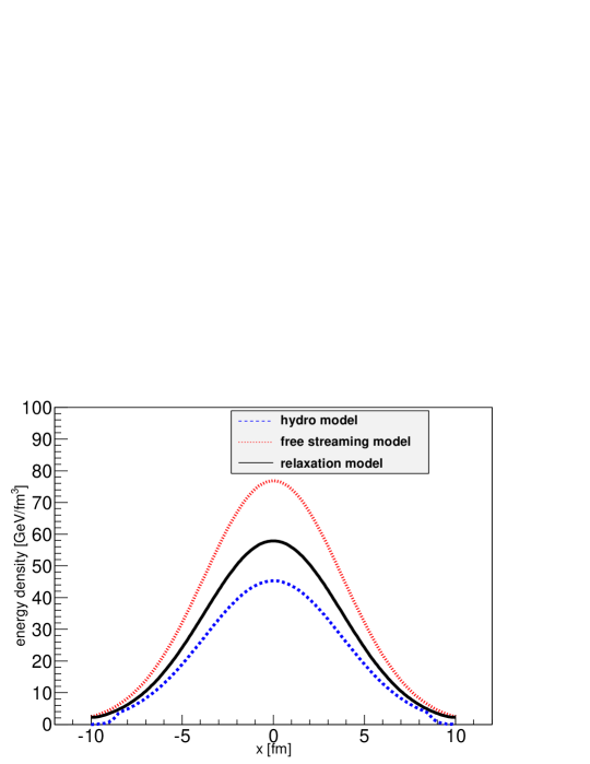
Figure 1: (Color online). The energy density distribution along axis $x$, ($y=0$) in transverse plane for central rapidity slice at $\tau=\tau_{\text{th}}=1.0$ fm/c for the following conditions of the relaxation evolution: $\tau_{0}=0.1$ fm/c, the Gaussian initial transverse energy density profile, $\lambda=1$, EoS: $p=\epsilon/3$, $\tau_{\text{rel}}=0.5$ fm/c, the target energy-momentum tensor corresponds to ideal hydrodynamics.

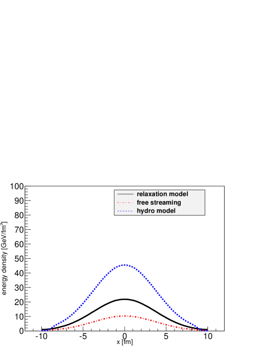
Figure 2: (Color online). The energy density distribution at $\tau=\tau_{\text{th}}=1.0$ fm/c under the same conditions as in Fig. 1, but with large initial anisotropy, $\lambda=0.01$.

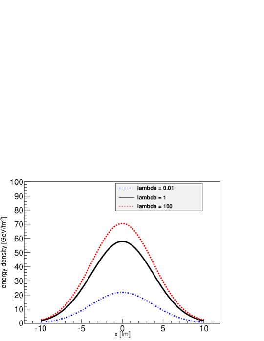
Figure 3: (Color online). The comparison of the results of the relaxation model for energy density distributions at $\tau=\tau_{\text{th}}=1.0$ fm/c for momentum isotropic, $\lambda=1$, and very anisotropic, $\lambda=0.01$, $\lambda=100$ initial states under the same other conditions as in Fig. 1.

In Fig. 1 we present the energy densities for the relaxation model in comparison with the hydrodynamic model and the free streaming evolution for isotropic initial state, $\lambda=1$, with the equation of state $p=\epsilon/3$. As one can see from Fig. 1, the final (at the thermalization time $\tau=\tau_{\text{th}}=1$ fm/c) energy density in RM is in between the corresponding results for HM (minimal values) and FS model (maximal values) cases. These results are expected because the relaxation evolution incorporates both HM- and FS- regimes, and the anisotropy parameter is chosen to be $\lambda=1>1/3$. Note that in any anisotropic case, i.e. $\lambda\neq 1$, which we start to discuss, the initial conditions for hydrodynamics at $\tau=\tau_{0}=0.1$ fm/c are taken in our analysis with the same initial energy density as at the anisotropic distribution, $\epsilon_{\text{hyd}}=\epsilon$, but with symmetric pressure $p_{\text{hyd}}=c_{0}^{2}\epsilon$, where $c_{0}^{2}=1/3$ everywhere in our analysis except for the specially defined cases. Figure 2 corresponds to the anisotropic case with $\lambda=0.01$, when the longitudinal “effective temperature” $\lambda_{\|}$ is much larger than the transverse one, $\lambda_{\|}>\lambda_{\bot}$. Again, the final energy densities at RM- regime reach intermediate values between the corresponding results for HM- and FS- cases. However, since now $\lambda<1/3$, the smallest values of the energy are reached at FS- regime and the maximal ones at HM- expansion. The detailed analysis of the RM-, HM- and FS- regimes in the vicinity of the point $\lambda=1/3$: $\lambda=(0.25,0.45)$ demonstrates the changing of sequence for different regimes at $\tau_{th}$, at the same time RM- energy density never coincides simultaneously with both HM- and FS- energy densities. Also, a coincidence of the RM final energy density with either the HM or the FS model one is accompanied by different pre-thermal flows in the corresponding pair. In Fig. 3 we compare the results of the relaxation model for the initial distributions, which are isotropic, $\lambda=1$, and strongly anisotropic, $\lambda=0.01$ and $\lambda=100$, in momentum space. The last case is associated typically with Color Glass Condensate (CGC) initial conditions parametr-2 . One can see that at the same initial densities at $\tau=0.1$ fm/c, the maximal energy density at the thermalization time $\tau=1$ fm/c is reached for the case with the smallest longitudinal pressure.

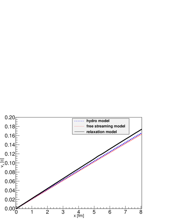
Figure 4: (Color online). The transverse velocity distribution at $\tau=\tau_{\text{th}}=1.0$ fm/c and $\lambda=1$ under the same conditions as in Fig. 1.

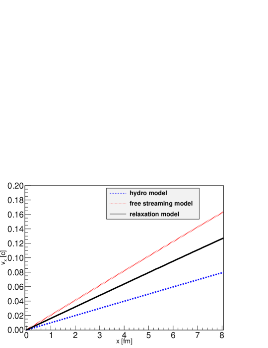
Figure 5: (Color online). The transverse velocity distribution at $\tau=\tau_{\text{th}}=1.0$ fm/c under the same conditions as in Figs. 1, 4 but softer EoS: $p=0.15\epsilon$.

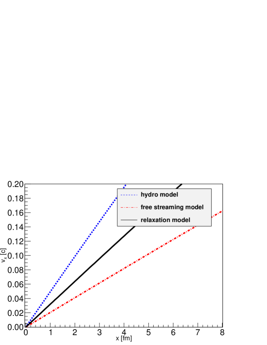
Figure 6: (Color online). The transverse velocity distribution at $\tau=\tau_{\text{th}}=1.0$ fm/c under the same conditions as in Figs. 1, 4 but harder EoS: $p=0.7\epsilon$.

The situation with the transverse collective velocities (Fig. 4) is not trivial even in the isotropic case, where the energy density value in RM is in between the ones in the FS model and HM. The reason is that there are two oppositely directed factors which act simultaneously to the transverse gradient of the hydrodynamic pressure that contributes to formation of the velocity field in the RM-regime. On the one hand, harder equation of state increases the gradient, but on the other hand, the hard equation of state could reduce it since more energy loss happens due to the fact that more work is done in the longitudinal direction by the system contained in some rapidity interval. We demonstrate such an interplay in Figs. 4, 5, and 6; the maximal final velocities are reached at $p_{\text{hyd}}=\epsilon/3$ in RM, at $p_{\text{hyd}}=0.15\epsilon$ in FS, and at $p_{\text{hyd}}=0.7\epsilon$ in HM.

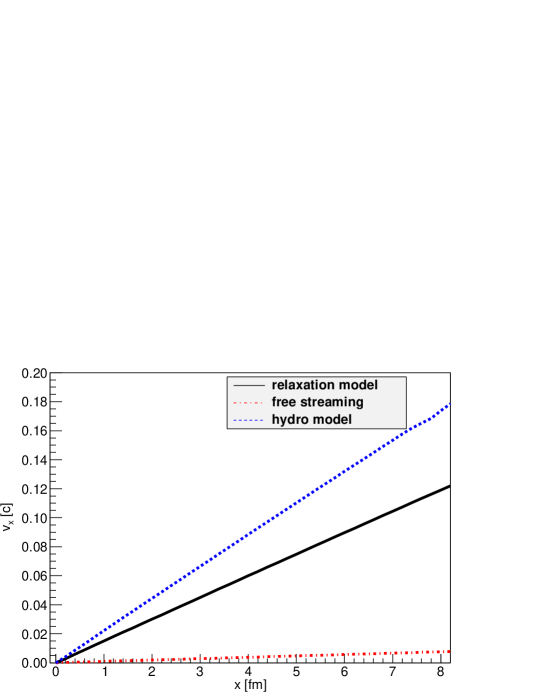
Figure 7: (Color online). The transverse velocity distribution at $\tau=\tau_{\text{th}}=1.0$ fm/c under the same conditions as in Figs. 1, 4, but with large initial anisotropy, $\lambda=0.01$.

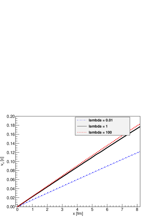
Figure 8: (Color online). The comparison of the results of the relaxation model for transverse velocity distributions at $\tau=\tau_{\text{th}}=1.0$ fm/c for isotropic, $\lambda=1$ and very anisotropic, $\lambda=0.01$, $\lambda=100$ initial states under the same other conditions as in Fig. 1.

In Fig. 7 the transverse velocities for initially very anisotropic states, $\lambda=0.01$ are presented. As opposed to the $\lambda=1$ regime, at small $\lambda<1/3$ the minimal pre-thermal flow develops in the case of the FS-regime and a maximal flow in the HM one. The RM-regime leads to an intermediate result. One can see the influence of the anisotropy on the RM results from Figs. 3, 8, where it is found that the energy densities and pre-thermal collective flows grow when the anisotropy parameter $\lambda$ increases. The reason is that the increase of $\lambda$ results in the decrease of the energy density loss rate for the FS-component during the boost-invariant expansion (see Eq. (20) and discussion there). As a result, the maximal energy densities and transverse gradient of the FS-component are larger during the relaxation process when $\lambda$ is larger. In its turn the transverse gradient of particle or/and energy densities define the transverse flow at free streaming process early , hbt-ic : It grows when the gradient increases.

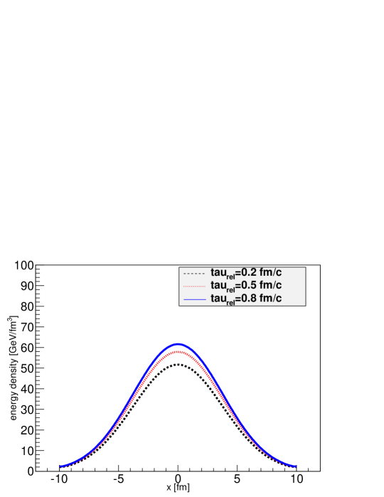
Figure 9: (Color online). The comparison of the energy density distributions at different $\tau_{\text{rel}}=0.2,0.5,0.8$ fm/c under the same other conditions as in Fig. 1.

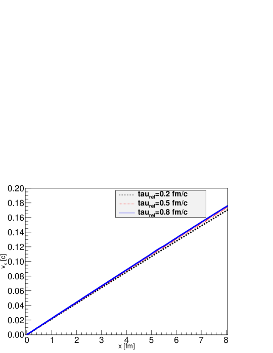
Figure 10: (Color online). The comparison of the transverse velocity distributions at different $\tau_{\text{rel}}=0.2,0.5,0.8$ fm/c under the same other conditions as in Figs. 1, 4.

To study how the rate of transition to hydrodynamics affects the energy densities and transverse velocities at the starting time of the hydrodynamic stage, we perform the simulations for different values of $\tau_{\text{rel}}$. The results are demonstrated in Figs. 9, 10 for $\lambda=1$ where one can see that the final transverse velocities are almost the same despite the different slopes of the transition, whereas the energy densities are larger if the rate of transition to hydrodynamics is smaller ($\tau_{\text{rel}}$ is larger). Such a behavior in the initially symmetric case is due to the free streaming regime, which dominates for longer time at larger $\tau_{\text{rel}}$. This also means that at $\lambda=1>1/3$ the energy density will be larger, cf. Eqs. (19) and (20). At the same time, by comparing the energy densities and transverse velocities, calculated in RM with $\tau_{\text{rel}}=0.8$ fm/c, that corresponds to rather abrupt transition to hydrodynamics near the end of the pre-equilibrium stage, with the ones calculated in FS, see Figs. 1, 4, one can find noticeable differences in the resulting energy density, which is smaller in RM than at the free streaming regime with $\lambda=1$. As a matter of fact, one cannot get the free streaming regime in the relaxation model.

It is important to emphasize now that both FS- and HM- regimes of expansions are not real limiting cases for the system evolution from an initial non-equilibrated (NEQ) state to a final equilibrated (EQ) one. At the same initial energy density profile, for any allowed parameters: $\tau_{0},\tau_{\text{th}}$ and $\tau_{\text{rel}}$, such “limiting” energy-momentum tensors cannot be reached. Formally, basic boundary equalities (6) prevent such a possibility. The physical reason is that the structures of the energy-momentum tensor are different for EQ- and NEQ- states. As we have discussed above, both the final energy density and transverse velocity profile in relaxation model do not coincide simultaneously with analogous values reached at FS- or HM- regimes, for any value of the anisotropy parameter $\lambda$. In the particular case of isotropic initial state ($\lambda=1$), the energy-momentum tensor in the free streaming evolution acquires specific (non-viscous) non-equilibrium structure with the energy density higher than in the case of any continuous transition to hydrodynamics demonstrated at Fig. 9. The reason is that one cannot simply ignore the non-diagonal terms in the energy-momentum tensor that are developing at free streaming evolution hbt-ic , and diagonalize the tensor “suddenly” at, say, $\tau=\tau_{\text{th}}=1$ fm/c by using Landau matching conditions, because then the energy-momentum conservation is violated. Thereby, the continuous interpolation between arbitrarily anisotropic initial state and hydrodynamical regime at some later time, provided by the relaxation model, does not imply “continuous interpolation” between the two “limiting” types of the matter evolutions: free streaming and hydrodynamical.

Another important point, which we outline here, is the initialization of viscous hydrodynamics by means of the relaxation model. The relaxation model equations (13) include the Israel-Stewart viscous hydrodynamical formalism, and the corresponding viscous hydrodynamic code Karp is modified to solve the relaxation model equations. We keep bulk pressure $\Pi=0$ everywhere during the evolution, by default use zero initial values for the shear stress tensor, $\pi^{\mu\nu}(\tau_{0})=0$, and use anzatz for the relaxation time of the shear stress tensor: $\tau_{\pi}=5\eta/(sT)$. In the viscous case one also needs to specify the temperature and entropy density from the equation of state. Therefore for the viscous case we always use the EoS for a relativistic massless gas of quarks and gluons, $p=\epsilon/3$, which results in the following relation for energy density:

$$\epsilon=\left(\frac{7}{4}g_{l}n_{f}+g_{g}\right)\frac{\pi^{2}}{30}T^{4},$$ (21)

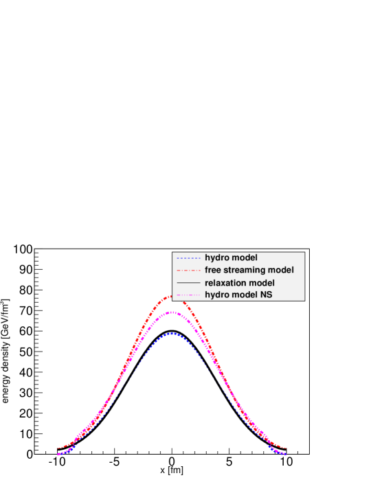
Figure 11: (Color online). The energy density distribution along axis $x$, ($y=0$) in transverse plane for central rapidity slice at $\tau=\tau_{\text{th}}=1.0$ fm/c for the following conditions of the relaxation evolution: $\tau_{0}=0.1$ fm/c, the Gaussian initial transverse energy density profile, $\lambda=1$, EoS: $p=\epsilon/3$, $\tau_{\text{rel}}=0.5$ fm/c, the target energy-momentum tensor corresponds to viscous hydrodynamics with $\eta/s$=0.1.

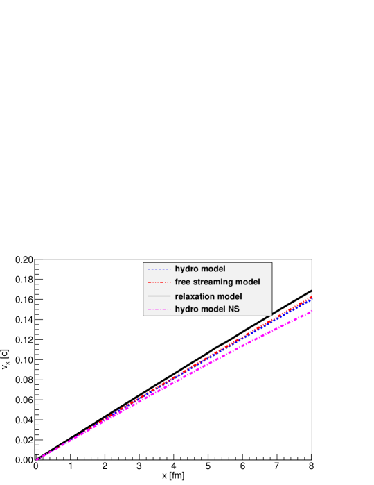
Figure 12: (Color online). The transverse velocity distribution at $\tau=\tau_{\text{th}}=1.0$ fm/c under the same conditions as in Fig. 11.

where $g_{l}=6$ ang $g_{q}=16$ are quark and gluon degeneracy factors, respectively, and we set the effective number of quark degrees of freedom $n_{f}=2.5$. Equation (21) as well assumes that the chemical potentials are zero. The entropy density is then extracted using the thermodynamical relation $\epsilon+p=Ts$. In the limiting Navier-Stokes case the fixed ratio of shear viscosity to entropy density $\eta/s=0.1$ is used. Also, in this case we perform calculations with initially isotropic momentum space distribution, $\lambda=1$. The results of RM are compared with the results of HM with initial shear viscous tensor $\pi^{\mu\nu}(\tau_{0})=0$, and with results of HM with initial shear viscous tensor equals to its limiting Navier-Stokes (NS) form, $\pi^{\mu\nu}(\tau_{0})=\pi^{\mu\nu}_{NS}$. The results are shown in Figs. 11 and 12, where the free streaming model calculations are added for comparison. The results of the relaxation model with zero viscous initial conditions are qualitatively similar to the results obtained in the relaxation model with the ideal fluid, for example, one can see from these figures that the relaxation model results in lower energy density in the center of the system and in higher transverse velocities as compared to the free streaming model. In the case of non-zero initial viscosity contribution at $\tau=\tau_{0}$ (NS limit), the final energy density in such a model is larger than in the relaxation model.

Finally we demonstrate that the viscous relaxation model, unlike “anisotropic hydrodynamics”, can be used not only for smooth initial energy density profiles, but also for bumpy anisotropic initial distributions at $\tau=\tau_{0}$. The set of such bumpy individual samples is used in event-by-event hydrodynamic analysis. To avoid misunderstanding, note that our aim here is not analysis which of the models: MC-Glauber, MC-KLN or IP-Glasma is more realistic for a data description (for this aim one needs to utilize a large number of individual samples and describe hadron momentum spectra and their $v_{n}$-coefficients), but only the demonstration of capabilities of the relaxation model. Thus, we pick randomly one particular (fluctuating) event corresponding to 20-30% central Pb+Pb collision at LHC energy generated with the GLISSANDO generator generator . The generator calculates the spatial distribution of sources, which fluctuates according to the statistical nature of the distributions of nucleons in the colliding nuclei, according to the Monte-Carlo Glauber model. The transverse coordinates of the sources correspond to either the centers of the wounded nucleons or the centers of the binary collisions of nucleons in colliding nuclei. The corresponding relative deposited strength (RDS) of each source is $(1-\alpha)/2$ if the source comes from a wounded nucleon, or $\alpha$ if it comes from a binary collision. We use the default value $\alpha=0.14$.

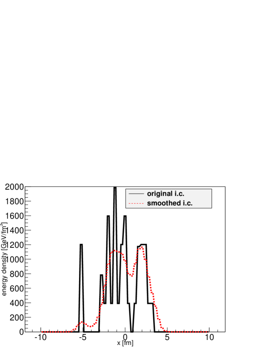
Figure 13: (Color online). The initial transverse distribution at $\tau=\tau_{0}=0.1$ fm/c of the energy density along $x$-axis ($y=0$) for the random single event produced by the GLISSANDO generator within Monte Carlo Glauber model. Smoothed distribution is shown by the dashed line.

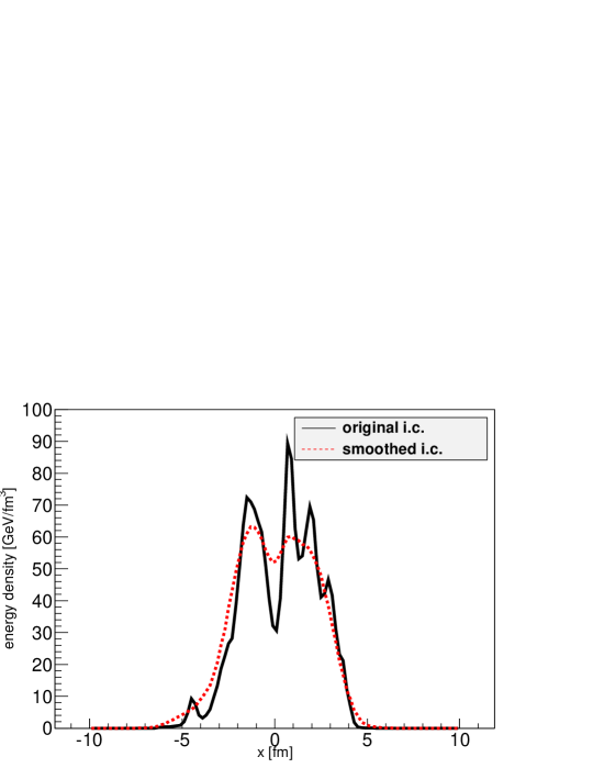
Figure 14: (Color online). The final energy density distribution along axis $x$ ($y=0$) in transverse plane for central rapidity slice at $\tau=\tau_{\text{th}}=1.0$ fm/c for GLISSANDO original and smeared initial energy density profiles shown in Fig. 13. The following conditions of the relaxation evolution are used: $\tau_{0}=0.1$ fm/c, $\lambda=1$, EoS: $p=\epsilon/3$, $\tau_{\text{rel}}=0.5$ fm/c, the target energy-momentum tensor corresponds to viscous hydrodynamics with $\eta/s=0.25$.

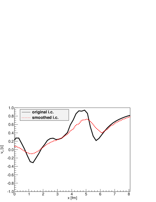
Figure 15: (Color online). The transverse velocity distribution for GLISSANDO original and smeared initial energy density profiles at $\tau=\tau_{\text{th}}=1.0$ fm/c under the same conditions as in Fig. 14.

One needs initial conditions, which are averaged within each cell, as a numerical input for the hydrodynamic or relaxation model. In order to get them, one can use one of standard outputs of GLISSANDO, which is a $2D$ histogram filled with RDS of all sources in the transverse plane. The default value of the bin size of the histogram is $s_{\text{GL}}=0.4$ fm. Formally it is similar to the coarse-graining procedure which is the basis of any macroscopic description (say, hydrodynamic) of a microscopic system. In fact, each hydrodynamic initial condition corresponds to many microscopic initial states with almost the same densities associated with the selected scale. So, if one wants to associate the single GLISSANDO event with further hydrodynamic evolution, the corresponding energy density distribution cannot be very inhomogeneous. Also, it is known that the viscosity parameters are related directly to the coarse-grained scale scale . At too small scales, the inhomogeneity of the medium can be so large (tends to the point-like one in the limiting case) that viscous hydrodynamics loses its applicability. To address this question we compare the results obtained for the (non-smeared) initial distribution described above with the results calculated for a smeared initial distribution. For the latter, we increase the bin size of the histogram from the default one, $s_{\text{GL}}=0.4$ fm, to $s_{\text{GL}}=0.7$ fm. To get the smeared initial distribution, we also distribute the energy from every individual cell to the transverse area centered around it, according to a Gaussian profile with a radius $\sigma=0.5$ fm. The non-smeared energy density profile, produced by GLISSANDO generator in the randomly selected single event, is demonstrated in Fig. 13 in comparison with the smeared one. Note that both bumpy initial distributions, original and smeared ones, are normalized to the same mean value $\bar{\epsilon}_{0}=1000$ GeV/fm³ of the energy density averaged in transverse plane within the central square with side $4$ fm. We use both, non-smeared and smeared profiles, instead of the Gaussian one (15) in Eq. (16). Then, using the original and smeared $r_{T}$-profiles, the corresponding initial phase-space densities $f(x,p)$, as well as the initial energy-momentum tensors, can be defined on an event-by-event basis. The results of the relaxation model for the randomly selected single event with corresponding initial energy density distributions in Fig. 13 are presented in Figs. 14 and 15 for the case of relatively large viscosity parameter, $\eta/s=0.25$, and $\lambda=1$. One can see the different level of inhomogeneity of initial conditions for hydrodynamics at $\tau_{\text{th}}=$1 fm/c with smeared and non-smeared initial states at $\tau=\tau_{0}$.

Simulations of $A+A$ collisions require initialization of the relaxation transport model for many such fluctuating initial states. The statistically relevant number of such events is of the order of event number $N$ that saturates the average value of initial conditions at $\tau_{0}$. It is worth noting that for the GLISSANDO event generator $N\approx 1000$. Calculation in the relaxation transport model of a single event, that includes also evaluation of the source term $T^{\mu\nu}_{\text{free}}(x)\partial_{;\mu}{\cal P}(\tau)$ in Eq. (13), takes about $4$ hours at one processor core. So, with parallel calculations ($100$ processors) the total time for event-by-event analysis of relativistic heavy ion collisions takes about one or two days.

The dependence of the hadron spectra and $v_{n}$ on the coarse-graining scale as well as connection between the scale and viscous parameters is the separate important topic which is beyond the scope of the present paper.

IV Summary

A reliable analysis of the properties of quark-gluon plasma and initial state of matter formed in relativistic heavy ion collisions requires the knowledge of the pre-thermal dynamics of the collisions that leads to thermalization of the system and its further hydrodynamic evolution. However, until now there has been no fully satisfactory framework to address dynamical aspects of isotropization and thermalization in nucleus-nucleus collisions. Hence a consistent match of a non-equilibrium initial state of matter with hydrodynamic approximation in such collisions remains an open question.

We have presented the results for hydrodynamical initial conditions obtained with the simulations of pre-equilibrium relaxation dynamics in the energy-momentum transport phenomenological model that was proposed in Ref. preth . Unlike the anisotropic hydrodynamics approach aniz , where the artificial concept of “anisotropic equilibrium” based on $0+1$ dimensional kinetics for specific class of anisotropy is utilized instead of Gibbs relations to close the system of evolutionary equations, this model does not have any additional assumptions and therefore can be applied for systems which are arbitrary anisotropic in momentum space as well as inhomogeneous in transverse plane. The latter is particularly important for the event-by-event hydrodynamical modeling of relativistic heavy ion collisions. We have calculated the initial conditions for the hydrodynamical evolution using initial states which can be initially isotropic or anisotropic in momentum space. The dependence of the target thermal state on the rates of conversion to hydrodynamical regime and different equations of state is presented as well. It allows us to study the influence of peculiarities of early initial state as well as pre-equilibrium dynamics on the energy densities and collective transverse velocities at the starting time of the hydrodynamical evolution.

In particular it is found that, with the same initial energy density, both final energy densities and pre-thermal transverse collective flows increase when the anisotropy parameter - the ratio of transverse pressure to longitudinal one, increases. Therefore the highest hydrodynamical energy densities and transverse velocities at thermalization time are reached at initial zero longitudinal pressure that corresponds the CGC-like initial state. Also, we found that for any relaxation time and initial momentum anisotropy, both the final energy density and transverse velocity profile in the relaxation model never coincide simultaneously with analogous values reached in the hydrodynamic model or at the free streaming regime. Therefore, continuous relaxation dynamics from an initially non-equilibrium state to an (almost) equilibrium one can not be properly approximated by the free streaming or hydrodynamic regime. The commonly used prescription of sudden thermalization of the free streaming pre-thermal evolution results in discontinuity in the energy-momentum tensor, which for free streaming has specific (non-viscous) non-equilibrium structure. This results in a breakdown of the energy and momentum conservation laws.

The peculiarities of the pre-thermal evolution also depend on the equation of state for the hydrodynamic component of the system. The two oppositely directed factors act simultaneously to the transverse gradient of the hydrodynamic pressure that contributes to formation of the transverse velocity field at relaxation evolution. On the one hand, harder equation of state increases the gradient, but on the other hand, the hard equation of state could reduce it since more energy loss happens due to more work is done in longitudinal direction by the system contained in some rapidity interval. As a result, the maximal transverse velocities are reached for isotropic initial state in the following cases: for a soft equation of state (EoS) at the free streaming evolution, for an ultra-hard EoS at the pure hydrodynamic expansion, and for an intermediate EoS for the relaxation evolution.

The developed relaxation model is also applied for the situations when the pre-thermal system relaxes to a close-to-equilibrium state described by viscous hydrodynamics. It is demonstrated that the viscous relaxation model can be utilized even with rather bumpy initial states, which allows one to use the model as a component of hydrodynamical event-by-event analysis.

The physically clear explanations of the results allow one to conjecture that although the presented results are model-dependent, it is plausible to assume that they reproduce general properties of the pre-equilibrium dynamics for anisotropic initial momentum distributions.

- (1) U. Heinz, J. Phys.: Conf. Ser. 455, 012044 (2013) [arXiv:1304.3634]; U. Heinz, R. Snellings, Annu. Rev. Nucl. Part. Sci. 63, 123 (2013) [arXiv:1301.2826]; C. Gale, S. Jeon, B. Schenke, Int. J. Mod. Phys. A 28, 1340011 (2013) [arXiv:1301.5893]; P. Huovinen, Int. J. Mod. Phys. E 22, 1330029 (2013) [arXiv:1311.1849]; H. Song, arXiv:1401.0079.
- (2) Yu.M. Sinyukov, S.V. Akkelin, Y. Hama, Phys. Rev. Lett. 89, 052301 (2002).
- (3) S.V. Akkelin, Y. Hama, Iu.A. Karpenko, Yu.M. Sinyukov, Phys. Rev. C 78, 034906 (2008); Yu.M. Sinyukov, S.V. Akkelin, Iu.A. Karpenko, Y. Hama, Acta Phys. Polon. B 40, 1025 (2009) [arXiv:0901.1576]; Yu.A. Karpenko, Yu.M. Sinyukov, J. Phys. G: Nucl. Part. Phys. 38, 124059 (2011) [arXiv:1107.3745]; Iu.A. Karpenko, Yu.M. Sinyukov, K. Werner, Phys. Rev. C 87, 024914 (2013).
- (4) Yu.M. Sinyukov, S.V. Akkelin, Iu.A. Karpenko, V.M. Shapoval, Advances in High Energy Physics, vol. 2013, Article ID 198928, 23 pages [http://dx.doi.org/10.1155/2013/198928].
- (5) P. Huovinen, H. Petersen, Eur. Phys. J. A 48, 171 (2012) [arXiv:1206.3371]; S. Pratt, Phys. Rev. C 89, 024910 (2014); D. Molnar, Z. Wolff, arXiv:1404.7850.
- (6) S.A. Bass et al., Prog. Part. Nucl. Phys. 41, 255 (1998); M. Bleicher et al., J. Phys. G 25, 1859 (1999).
- (7) B. Müller, A. Schäfer, Int. J. Mod. Phys. E 20, 2235 (2011) [arXiv:1110.2378]; J. Berges, K. Boguslavski, S. Schlichting, R. Venugopalan, Phys. Rev. D 89, 114007 (2014); J.-P. Blaizot, B. Wu, L. Yan, Nucl. Phys. A 930,139 (2014); O. DeWolfe, S.S. Gubser, C. Rosen, D. Teaney, Progr. Part. Nucl. Phys. 75, 86 (2014) [arXiv:1304.7794]; S.V. Akkelin, Yu.M. Sinyukov, Phys. Rev. C 89, 034910 (2014); X.-G. Huang, J. Liao, Int. J. Mod. Phys. E 23, 1430003 (2014) [arXiv:1402.5578]; R. Venugopalan, Nucl. Phys. A 928, 209 (2014); A. Kurkela, E. Lu, Phys. Rev. Lett. 113, 182301 (2014); J. Berges, B. Schenke, S. Schlichting, R. Venugopalan, Nucl. Phys. A 931, 348 (2014).
- (8) F. Gelis, E. Iancu, J. Jalilian-Marian, R. Venugopalan, Ann. Rev. Nucl. Part. Sci. 60, 463 (2010) [arXiv:1002.0333].
- (9) M. Alvioli, H.-J. Drescher, M. Strikman, Phys. Lett. B 680, 225 (2009); H. Holopainen, H. Niemi, K. J. Eskola, Phys. Rev. C 83, 034901 (2011); M. Alvioli, H. Holopainen, K. J. Eskola, M. Strikman, Phys. Rev. C 85, 034902 (2012).
- (10) D. Kharzeev, C. Lourenco, M. Nardi, H. Satz, Z. Phys. C 74, 307 (1997); D. Kharzeev, M. Nardi, Phys. Lett. B 507, 121 (2001); D. Kharzeev, E. Levin, Phys. Lett. B 523, 79 (2001); D. Kharzeev, E. Levin, M. Nardi, Phys. Rev. C 71, 054903 (2005).
- (11) B. Schenke, P. Tribedy, R. Venugopalan, Phys. Rev. Lett. 108, 252301 (2012); Phys. Rev. C 86, 034908 (2012).
- (12) T. Schäfer, Annu. Rev. Nucl. Part. Sci. 64, 125 (2014) [arXiv:1403.0653].
- (13) K. Huang, Statistical Mechanics (John Wiley Sons, Inc., New York - London, 1963); R. Balescu, Equilibrium and Nonequilibrium Statistical Mechanics (John Wiley Sons, Inc., New York - London - Sydney - Toronto, 1975); D. Zubarev, V. Morozov, and G. Röpke, Statistical Mechanics of Nonequilibrium Processes (Akademie Verlag, Berlin, 1996, 1997).
- (14) C. Cercignani and G.M. Kremer, The Relativistic Boltzmann Equation: Theory and Applications (Birkhäuser Verlag, Basel - Boston - Berlin, 2002).
- (15) M. Strickland, Nucl. Phys. A 926, 92 (2014); arXiv:1410.5786.
- (16) P. Romatschke and M. Strickland, Phys. Rev. D 68, 036004 (2003).
- (17) M. Martinez and M. Strickland, Phys. Rev. C 81, 024906 (2010); Nucl. Phys. A 848, 183 (2010).
- (18) W. Florkowski, R. Ryblewski, and M. Strickland, Nucl. Phys. A 916, 249 (2013); Phys. Rev. C 88, 024903 (2013).
- (19) L. Tinti, W. Florkowski, Phys. Rev. C 89, 034907 (2014); D. Bazow, U.W. Heinz, and M. Strickland, Phys. Rev. C 90, 054910 (2014); U. Heinz, D. Bazow, M. Strickland, Nucl. Phys. A 931, 920 (2014); L. Tinti, arXiv:1411.7268.
- (20) S.V. Akkelin, Yu.M. Sinyukov, Phys. Rev. C 81, 064901 (2010).
- (21) Yu.M. Sinyukov, Acta Phys. Polon. B 37, 3343 (2006); Yu.M. Sinyukov, A.N. Nazarenko, Iu.A. Karpenko, Acta Phys. Polon. B 40, 1109 (2009).
- (22) Iu. Karpenko, P. Huovinen, M. Bleicher, Comput. Phys. Commun. 185, 3016 (2014) [arXiv:1312.4160].
- (23) R. Ryblewski, W. Florkowski, Acta Phys. Polon. B 42, 115 (2011).
- (24) Yu.M. Sinyukov, Iu. A. Karpenko and A. V. Nazarenko, J. Phys. G: Nucl. Part. Phys. 35, 104071 (2008); Iu.A. Karpenko, Yu.M. Sinyukov, Phys. Rev. C 81, 054903 (2010).
- (25) M. Gyulassy, Iu. Karpenko, A.V. Nazarenko, Yu.M. Sinyukov, Braz. Journ. of Phys. 37, 1031 (2007).
- (26) W. Broniowski, M. Rybczyński, P. Bożek, Comput. Phys. Commun. 180, 69 (2009) [arXiv:0710.5731].
- (27) Ph. Mota, T. Kodama, J. Takahashi, R. Derradi de Souza, Eur. Phys. J. A 48, 165 (2012).