Relativistic Fe $\mathbf{K\alpha}$ Line Revealed in the Composite X-ray Spectrum of Narrow Line Seyfert 1 Galaxies — do their black holes have averagely low or intermediate spins?

Abstract

While a broad profile of the Fe $\mathrm{K\alpha}$ emission line is frequently found in the X-ray spectra of typical Seyfert galaxies, the situation is unclear in the case of Narrow Line Seyfert 1 galaxies (NLS1s)—an extreme subset which are generally thought to harbor less massive black holes with higher accretion rates. In this paper, the ensemble property of the Fe $\mathrm{K\alpha}$ line in NLS1s is investigated by stacking the X-ray spectra of a large sample of 51 NLS1s observed with XMM-Newton. The composite X-ray spectrum reveals a prominent, broad emission feature over 4–7 keV, characteristic of the broad Fe $\mathrm{K\alpha}$ line. In addition, there is an indication for a possible superimposing narrow (unresolved) line, either emission or absorption, corresponding to Fe XXVI or Fe XXV, respectively. The profile of the broad emission feature can well be fitted with relativistic broad-line models, with the line energy consistent either with 6.4 keV (i.e., neutral Fe) or with 6.67 keV (i.e., highly ionized Fe), in the case of the narrow line being emission and absorption, respectively. Interestingly, there are tentative indications for low or intermediate values of the average spins of the black holes ($a<0.84$), as inferred from the profile of the composite broad line. If the observed feature is indeed a broad line rather than resulting from partial covering absorption, our results suggest that a relativistic Fe line may in fact be common in NLS1s; and there are tentative indications that black holes in NLS1s may not spin very fast in general.

1 Introduction

The Fe $\mathrm{K\alpha}$ emission is the most important line feature in the X-ray spectra of Seyfert galaxies (Pounds et al., 1990). Such a narrow line is commonly found among Seyfert galaxies (Nandra & Pounds, 1994; Yaqoob & Padmanabhan, 2004; Zhou & Wang, 2005). In addition, there is also observational evidence for a broad Fe $\mathrm{K\alpha}$ line in some active galactic nuclei (AGN), whose archetypes include MCG-6-30-15 (Tanaka et al., 1995; Fabian et al., 2002; , Miniutti et al.2007), NGC 3516 (Turner et al., 2002; Markowitz et al., 2006), 1H0707-495 (Fabian et al., 2009) and others (Nandra et al., 2007; Miller, 2007). The broad Fe $\mathrm{K\alpha}$ line is generally thought to originate from ‘cold’ gas in the proximity of the supermassive black hole, such as the accretion disc, via the K-shell fluorescence process, illuminated by X-rays from a primary X-ray source, such as a postulated hot corona above the accretion disc (Fabian et al., 1989, alternative explanations have also been suggested, however; see Miller et al. 2008 for the absorption-origin model and Tatum et al. 2012 for the Compton-thick wind model). In the presence of strong gravitational field, the line can be significantly broadened, shifted and distorted due to the effects of both General and Special Relativity, including Doppler boosting, gravitational redshift and the transverse Doppler effect. The emergent line has a characteristic shape and the exact profile is determined by the physical properties of the disc and the black hole. The energy of the red wing of the broad line, redshifted due mainly to the gravitational redshift effect, is determined by the inner radius of the accretion disc, which is commonly thought to be at the innermost stable circular orbit (ISCO). The location of the ISCO is strongly dependent on the spin of the black hole; it is at 6 $r_{\rm g}$ ($r_{\rm g}=GM/c^{2}$, gravitational radius) for a non-spinning black hole and 1.24 $r_{\rm g}$ for a maximally spinning black hole (dimensionless spin parameter $a=0.998$). The energy and profile of the broad line are also dependent on the ionization state and the inclination of the accretion disc (Ross & Fabian, 1993; Fabian et al., 2000). As such, the profile of a relativistic broad Fe $\mathrm{K\alpha}$ line can be used to constrain the spin of the black hole (Brenneman & Reynolds, 2006; Dauser et al., 2010; Risaliti et al., 2013), as well as to probe the physical environment in the vicinity of the black hole.

There have been extensive studies for characterizing the Fe $\mathrm{K\alpha}$ line properties of Seyfert galaxies in the literature. For instance, Nandra et al. (1997) analyzed the spectra of 18 Seyfert 1 galaxies observed with ASCA, and concluded that nearly 75 per cent objects of their sample show evidence of broad lines. Based on XMM-Newton spectra of a sample of 26 Seyfert galaxies, Nandra et al. (2007) found that almost all the spectra show a narrow ‘core’ at 6.4 keV while $\sim$45 per cent of the spectra can be best fitted with a relativistic blurred reflection model. de La Calle Pérez et al. (2010) systematically and uniformly analyzed a collection of 149 radio-quiet Type 1 AGN observed by XMM-Newton. They found that about 36 per cent of sources in their flux-limited sample show strong evidence of a relativistic Fe $\mathrm{K\alpha}$ line with an average line equivalent width ($EW$) of the order of 100 eV, and this fraction can be considered as a lower limit in the wider AGN population. By analysing the spectra of 46 objects observed with Suzaku, Patrick et al. (2012) found that almost all the objects reveal a narrow Fe $\mathrm{K\alpha}$ line and 50 per cent of the sample show a statistically significant relativistic Fe $\mathrm{K\alpha}$ line with a mean equivalent width $\sim$$96\pm 10$ eV. It is generally accepted that a broad Fe $\mathrm{K\alpha}$ line is frequently presented in Seyfert galaxies.

For individual objects, however, it requires a large number of X-ray photons collected at high energies ($\gtrsim 4$ keV) to determine accurately the continuum spectrum and to reveal unambiguously the Fe $\mathrm{K\alpha}$ line profile (de La Calle Pérez et al., 2010). This is often unrealistic for the majority of AGN given the limited observing time available in practice, except for a small number of the brightest ones. Alternatively, spectral stacking is an effective way to obtain a composite spectrum with very high signal-to-noise for a certain class of objects. By stacking the X-ray spectra of 53 type 1 and 41 type 2 AGN, Streblyanska et al. (2005) found broad relativistic Fe $\mathrm{K\alpha}$ lines with an $EW$ of 600 eV and 400 eV for type 1 and type 2 AGN, respectively. Corral et al. (2008) introduced a sophisticated stacking method and applied it to an AGN sample (mostly quasars) observed with XMM-Newton; they found a significant unresolved narrow Fe $\mathrm{K\alpha}$ line around $\sim$6.4 keV with an $EW\sim 90$ eV in the stacked spectrum, and only an indication for a broad Fe $\mathrm{K\alpha}$ line which is not significant statistically. Using a sample of 248 AGN with a wide redshift range, Chaudhary et al. (2012) analyzed the average Fe $\mathrm{K\alpha}$ line profile using two fully independent rest-frame stacking methods. They found that the average Fe $\mathrm{K\alpha}$ profile can be best fitted by a combination of a narrow and a broad line with an $EW$ of $\sim$30 eV and $\sim$100 eV respectively. Iwasawa et al. (2012) performed spectral stacking analysis of the XMM-COSMOS field to investigate the Fe $\mathrm{K\alpha}$ line properties of AGN beyond redshift $z>1$; for type 1 AGN, they found a broad Fe emission line at a low significant level ($\sim$2$\sigma$) for only sub-samples of low X-ray luminosities ($<3\times 10^{44}$ ergs s^-1) or intermediate Eddington ratios ($\lambda\sim 0.1$); for type 2 AGN, no significant broad Fe line is found.

For Narrow Line Seyfert 1 galaxies (NLS1s), the situation is far less clear, however, given that the broad Fe line is detected at high significance in a few objects only. NLS1s are a subset of AGN defined as having the full width at half maximum (FWHM) of their broad Balmer lines smaller than $\sim$$2000\rm{~{}km~{}s^{-1}}$ (Osterbrock & Pogge, 1985; Goodrich, 1989). Compared to typical Seyferts—broad-line Seyfert 1 galaxies (BLS1s), NLS1s generally show strong $\mathrm{Fe\,{II}}$ and weak $\mathrm{[O\,III]}$ emission (Véron-Cetty et al., 2001), steep soft X-ray spectra (Puchnarewicz et al., 1992; Wang et al., 1996; Grupe, 2004), and sometimes extreme X-ray variability (Leighly, 1999; Grupe, 2004). It is generally accepted that NLS1s have higher accretion rates close to the Eddington rate (Boroson & Green, 1992) and relatively small black hole masses than BLS1s (Boroson, 2002; Komossa & Xu, 2007). It has also been suggested that NLS1s might be young AGN with fast growing black holes at an early stage of evolution (e.g., Mathur, 2000). Their accretion process may proceed in a somewhat different form from the standard thin disc, e.g., a slim disc as suggested to dominate in the regime of high accretion rates close to the Eddington rate or even higher (Abramowicz et al., 1988; Mineshige et al., 2000). NLS1s may represent the extreme form of Seyfert activity and may provide a new insight into the growth of massive black holes and accretion physics (Komossa, 2008).

As far as the broad Fe $\mathrm{K\alpha}$ line is concerned, somewhat contradictory results have been reported in the literature. There are a few well-studied NLS1s showing apparently a broad Fe $\mathrm{K\alpha}$ emission line, including 1H 0707-495 (Fabian et al., 2009) and SWIFT J2127.4+5654 (Miniutti et al., 2009; Marinucci et al., 2014). In an X-ray study of a large sample of AGN in de La Calle Pérez et al. (2010, see also ), broad Fe $\mathrm{K\alpha}$ lines were detected in 4 out of 30 ($\sim$13 per cent) NLS1s in the full sample and in 2 out of 4 in the flux limited sample. Ai et al. (2011) studied the X-ray properties of a sample of 13 extreme NLS1s that have very small broad-line widths ($<1200\rm{~{}km~{}s^{-1}}$) and found evidence for significant Fe $\mathrm{K\alpha}$ lines in none of the objects. Zhou & Zhang (2010) found that narrow Fe $\mathrm{K\alpha}$ emission lines in NLS1s are systematically much weaker than those in BLS1s. It should be noted that in previous studies of NLS1s, the X-ray spectra of individual objects are mostly of low S/N ratios at energies around the Fe $\mathrm{K\alpha}$ line and higher, partly due to the relatively steep continua above 2 keV. This results in low photon counts, and hence poorly determined continuum and low S/N, around the Fe $\mathrm{K\alpha}$ line region. It is not known whether a broad Fe $\mathrm{K\alpha}$ line is commonly present in NLS1s as a population. Furthermore, the detection of relativistic Fe $\mathrm{K\alpha}$ lines at high significance would render possible diagnostics to the spin of black holes in NLS1s. In this paper, we investigate the ensemble property of the Fe $\mathrm{K\alpha}$ line of NLS1s by stacking the X-ray spectra of a large sample of NLS1s observed with XMM-Newton. We use the cosmological parameters $H_{0}=70\,\mathrm{km\,s^{-1}\,Mpc^{-1}}$, $\Omega_{\mathrm{M}}=0.27$ and $\Omega_{\Lambda}=0.73$. All quoted errors correspond to the 90 per cent confidence level unless specified otherwise.

Figure 1: Left: Distribution of 2-10 keV rest-frame luminosity (MOS and PN) of the sample objects. Right: Distribution of 2-10 keV net photon counts.

Table 1: Basic parameters of the XMM-Newton sample

Object name	R.A.	D.E.C	Obs_ID	Redshift	EPIC MOS				EPIC PN			NH	FWHM(H$\beta$)	Ref.
	J2000.0	J2000.0			Exposure	Counts Rate	$f_{2-10~{}\rm{keV}}$		Exposure	Counts Rate	$f_{2-10~{}\rm{keV}}$
(1)	(2)	(3)	(4)	(5)	(6)				(7)			(8)	(9)	(10)
MARK 335	00 06 19.52	+20 12 10.5	0101040101	0.026	33.68	1.197	1.43E-11		28.47	1.631	1.33E-11	3.56	$1710\pm 140$	1
	…	…	0510010701	…	20.02	0.203	3.41E-12		15.56	0.290	2.98E-12	…	…	1
I Zw 1	00 53 34.94	+12 41 36.2	0110890301	0.059	—	—	—		18.22	0.999	8.18E-12	4.76	$1240$	2
SDSS J010712+140844	01 07 12.04	+14 08 45.0	0305920101	0.077	26.88	0.017	2.19E-13		16.02	0.024	1.62E-13	3.44	$787\pm 31$	3
MARK 359	01 27 32.55	+19 10 43.8	0112600601	0.017	—	—	—		6.84	0.629	5.30E-12	4.26	$900$	4
RXS J01369-3510	01 36 54.40	-35 09 52.0	0303340101	0.289	49.86	0.065	7.95E-13		38.99	0.095	8.22E-13	2.08	$1320$	5
PHL 1092	01 39 55.75	+06 19 22.5	0110890901	0.396	21.08	0.010	1.23E-13		14.80	0.016	1.23E-13	3.57	$1790$	2
RX J0306.6+0003	03 06 39.58	+00 03 43.2	0142610101	0.107	52.03	0.058	8.21E-13		40.30	0.081	7.94E-13	6.31	$1904\pm 51$	3
RXS J03232-4931	03 23 15.35	-49 31 06.7	0140190101	0.071	—	—	—		24.90	0.153	1.30E-12	1.34	$2075\pm 70$	5
RXS J04397-4540	04 39 44.84	-45 40 42.0	0204090101	0.224	27.92	0.008	1.28E-13		21.91	0.012	9.97E-14	0.91	$2105\pm 100$	5
PKS 0558-504	05 59 47.38	-50 26 52.4	0116700301	0.137	5.34	0.668	8.11E-12		—	—	—	3.37	$1250$	6
	…	…	0117500201	…	7.91	1.064	1.26E-11		—	—	—	…	…	6
	…	…	0137550201	…	14.02	0.800	9.90E-12		10.59	1.191	1.04E-11	…	…	6
	…	…	0137550601	…	—	—	—		10.22	2.436	2.10E-11	…	…	6
IRAS 06269-0543	06 29 24.67	-05 45 29.6	0153100601	0.117	7.42	0.175	2.23E-12		2.59	0.271	2.51E-12	34.60	$\star$	7,8
SDSS J081053+280610	08 10 53.75	+28 06 11.0	0152530101	0.285	27.02	0.004	4.66E-14		16.21	0.007	6.46E-14	2.89	$1212\pm 78$	3
SDSS J082433+380013	08 24 33.33	+38 00 13.1	0403760201	0.103	20.35	0.005	5.78E-14		14.00	0.009	5.79E-14	4.06	$780\pm 53$	3
SDSS J082912+500652	08 29 12.80	+50 06 52.0	0303550901	0.043	2.98	0.051	4.75E-13		—	—	—	4.08	$603\pm 21$	3
SBS 0919+515	09 22 47.03	+51 20 38.0	0300910301	0.160	21.07	0.027	3.37E-13		10.17	0.033	2.58E-13	1.33	$1132\pm 27$	3
MARK 110	09 25 12.87	+52 17 10.5	0201130501	0.035	46.12	1.713	2.49E-11		—	—	—	1.30	$1760\pm 50$	1
SDSS 094057+032401	09 40 57.20	+03 24 01.2	0306050201	0.061	26.27	0.015	4.58E-13		22.29	0.020	4.00E-13	3.20	$1119\pm 95$	3
SDSS 094404+480646	09 44 04.41	+48 06 46.6	0201470101	0.392	25.36	0.008	1.04E-13		11.92	0.010	9.37E-14	1.18	$1583\pm 26$	3
MARK 1239	09 52 19.10	-01 36 43.5	0065790101	0.020	9.27	0.015	5.52E-13		—	—	—	3.69	$1075$	4
ACIS J10212+0421	10 23 48.44	+04 05 53.7	0108670101	0.099	53.12	0.003	7.11E-14		46.06	0.004	3.95E-14	2.53	$696$	9,10
KUG 1031+398	10 34 38.60	+39 38 28.2	0109070101	0.042	12.65	0.074	7.99E-13		3.34	0.102	8.23E-13	1.31	$935$	4
	10 34 38.60	+39 38 28.2	0506440101	…	87.28	0.076	8.23E-13		72.67	0.107	8.15E-13	…	…	4
SDSS 104613+525554	10 46 13.73	+52 55 54.3	0200480201	0.503	18.37	0.010	1.25E-13		7.24	0.015	1.32E-13	1.16	$2053\pm 91$	3
SDSS 112328+052823	11 23 28.12	+05 28 23.3	0083000301	0.101	30.53	0.014	1.78E-13		25.53	0.022	2.09E-13	3.70	$1851\pm 62$	3
SDSS J11401+0307	11 40 08.71	+03 07 11.4	0305920201	0.081	40.22	0.025	2.76E-13		33.83	0.031	2.30E-13	1.91	$675\pm 41$	3
PG 1211+143	12 14 17.66	+14 03 13.3	0112610101	0.081	—	—	—		48.84	0.325	2.78E-12	2.74	$1860$	2
	…	…	0208020101	…	41.07	0.258	3.30E-12		32.94	0.350	3.05E-12	…	…	2
	…	…	0502050101	…	49.48	0.358	4.37E-12		44.07	0.468	3.88E-12	…	…	2
	…	…	0502050201	…	33.00	0.379	4.71E-12		25.71	0.507	4.20E-12	…	…	2
SDSS 121948+054531	12 19 48.94	+05 45 31.7	0056340101	0.114	29.56	0.011	2.17E-13		—	—	—	1.75	$1788\pm 102$	3
	…	…	0502120101	…	84.76	0.013	2.22E-13		68.18	0.015	1.97E-13	…	…	3
SDSS 123126+105111	12 31 26.45	+10 51 11.4	0306630101	0.304	68.07	0.003	7.08E-14		56.46	0.003	3.50E-14	2.31	$957\pm 23$	3
	…	…	0306630201	…	91.88	0.003	7.03E-14		81.51	0.003	4.89E-14	…	…	3

Table 1: Continue

Object name	R.A.	D.E.C	Obs_ID	Redshift	EPIC MOS				EPIC PN			NH	FWHM(H$\beta$)	Ref.
	J2000.0	J2000.0			Exposure	Counts Rate	$f_{2-10~{}\rm{keV}}$		Exposure	Counts Rate	$f_{2-10~{}\rm{keV}}$
(1)	(2)	(3)	(4)	(5)	(6)				(7)			(8)	(9)	(10)
SDSS 123748+092323	12 37 48.50	+09 23 23.2	0504100601	0.125	—	—	—		17.63	0.006	5.24E-13	1.48	$968\pm 74$	3
WAS 61	12 42 10.60	+33 17 02.6	0202180201	0.044	76.86	0.425	5.29E-12		56.54	0.568	4.69E-12	1.35	$1900\pm 150$	5
	…	…	0202180301	…	11.71	0.356	4.57E-12		9.16	0.480	4.06E-12	…	…	5
SDSS 124319+025256	12 43 19.98	+02 52 56.2	0111190701	0.087	59.64	0.012	4.32E-13		—	—	—	1.92	$1354\pm 59$	3
PG 1244+026	12 46 35.25	+02 22 08.8	0051760101	0.048	—	—	—		1.27	0.307	2.32E-12	1.87	$740$	4
SDSS 134351+000434	13 43 51.13	+00 04 38.0	0202460101	0.074	26.05	0.006	5.11E-13		20.47	0.006	1.22E-13	1.89	$2106\pm 73$	3
SDSS J134452+000520	13 44 52.91	+00 05 20.2	0111281501	0.087	6.95	0.015	2.34E-13		—	—	—	1.89	$1997\pm 38$	3
IRAS 13224-3809	13 25 19.38	-38 24 52.7	0110890101	0.066	61.22	0.044	3.53E-12		51.40	0.063	5.01E-13	5.34	$650$	2
SDSS 133141-015212	13 31 41.03	-01 52 12.5	0112240301	0.145	32.47	0.007	3.45E-12		24.40	0.009	2.09E-13	2.36	$1192\pm 42$	3
IRAS 13349+2438	13 37 18.73	+24 23 03.4	0402080201	0.108	32.83	0.288	2.30E-12		—	—	—	1.02	$2200$	11
	…	…	0402080301	…	58.58	0.275	6.27E-14		—	—	—	…	…	11
	…	…	0402080801	…	10.19	0.177	5.10E-13		—	—	—	…	…	11
2E 1346+2646	13 48 34.95	+26 31 09.9	0097820101	0.059	43.13	0.061	9.85E-13		34.34	0.085	8.69E-13	1.18	$1235^{a}$	4
	…	…	0109070201	…	54.76	0.035	7.11E-13		48.79	0.016	4.12E-13	…	…	4
SDSS J13574+6525	13 57 24.51	+65 25 05.9	0305920301	0.106	20.69	0.020	2.20E-13		15.94	0.030	2.54E-13	1.36	$737\pm 41$	3
	…	…	0305920601	…	14.83	0.020	2.49E-13		11.99	0.033	2.73E-13	…	…	3
UM 650	14 15 19.50	-00 30 21.6	0145480101	0.135	18.81	0.007	2.12E-13		13.66	0.009	1.06E-13	3.25	$1045\pm 27$	3
Zw 047.107	14 34 50.63	+03 38 42.6	0305920401	0.029	21.44	0.012	1.65E-13		17.34	0.016	1.39E-13	2.43	$1089^{a}$	12
MARK 478	14 42 07.46	+35 26 22.9	0107660201	0.079	24.67	0.240	2.72E-12		13.55	0.316	2.55E-12	1.05	$1270$	4
PG 1448+273	14 51 08.76	+27 09 26.9	0152660101	0.065	21.09	0.179	2.08E-12		17.91	0.242	1.94E-12	2.78	$1050$	4
IRAS 15091-2107	15 11 59.80	-21 19 01.7	0300240201	0.045	12.88	0.614	8.93E-12		5.02	0.877	7.95E-12	8.32	$1480$	13
SDSS 154530+484609	15 45 30.24	+48 46 09.1	0153220401	0.400	7.97	0.016	1.86E-13		—	—	—	1.64	$1821\pm 24$	3
	…	…	0505050201	…	6.13	0.028	3.75E-13		3.28	0.038	3.26E-13	…	…	3
	…	…	0505050701	…	6.12	0.022	2.35E-13		—	—	—	…	…	3
MARK 493	15 59 09.63	+35 01 47.5	0112600801	0.031	—	—	—		8.43	0.447	3.66E-12	2.11	$740$	4
KAZ 163	17 46 59.13	+68 36 27.8	0300910701	0.063	11.66	0.096	2.20E-12		7.69	0.115	2.23E-12	4.06	$1600$	14
PKS 2004-447	20 07 55.18	-44 34 44.3	0200360201	0.240	34.33	0.070	9.44E-13		25.17	0.094	8.73E-13	3.17	$1447$	15
MARK 896	20 46 20.87	-02 48 45.3	0112600501	0.026	10.44	0.321	3.91E-12		7.19	0.426	3.64E-12	3.39	$1135$	4
XMM J20584-4236	20 58 29.91	-42 36 34.3	0081340401	0.232	14.60	0.025	2.92E-13		7.19	0.037	3.09E-13	3.31	$\star$	16
II Zw 177	22 19 18.53	+12 07 53.2	0103861201	0.082	—	—	—		7.96	0.121	9.01E-13	4.90	$2080^{a}$	17,18
HB89 2233+134	22 36 07.68	+13 43 55.3	0153220601	0.326	8.68	0.044	6.18E-13		6.35	0.057	4.83E-13	4.51	$1840\pm 36$	3

The columns are: (1) object name; (2) and (3) position in J2000; (4):observation ID; (5) redshift; (6)(7) exposure (in units of kiloseconds), 2-10 keV counts rate and flux for EPIC MOS and PN; (8) Galactic column density; (9)FWHM of H$\beta$; (10) reference for the FWHM of H$\beta$, where 1: Grupe et al. (2004), 2: Leighly (1999), 3: Zhou et al. (2006), 4: Véron-Cetty et al. (2001), 5: Grupe et al. (1999), 6: Corbin (1997), 7: Véron-Cetty & Véron (2006), 8: Moran et al. (1996), 9: Hornschemeier et al. (2005), 10: Greene & Ho (2007), 11: Grupe et al. (1998), 12: Greene & Ho (2004), 13:Boller et al. (1996), 14: Haddad & Vanderriest (1991), 15: Oshlack et al. (2001), 16: Caccianiga et al. (2004), 17: Appenzeller et al. (1998), 18: Xu et al. (2003); (10) 2XMMcata-DR3 name

—: no data

$a$: measured using broad H$\alpha$ line.

$\star$: identified as NLS1s in the reference without giving the detail of the FWHM(H$\beta$)

2 Sample

We compiled a sample of NLS1s that have XMM-Newton observations from two NLS1s catalogues. The first by far is the largest NLS1s sample ($\sim$2000) selected from the SDSS DR3 by Zhou et al. (2006), which is homogeneously selected with well measured optical spectrometric parameters. The second includes NLS1s from the AGN catalogue compiled by Véron-Cetty & Véron (2006) comprising about 400 objects collected from the literature. We searched for XMM observational data from the XMM archive that are included in the Second XMM-Newton Serendipitous Source Catalogue (2XMMi-DR3, , Watson et al.2009). We selected those having more than 100 net source counts detected with either the EPIC PN or the combined MOS detectors in the 2-10 keV band. Three objects are excluded that are previously known to show a significant broad Fe $\mathrm{K\alpha}$ line, namely, 1H 0707-495, Mrk 766, and NGC 4051. The sample includes 51 NLS1s that have a total of 68 observations. A small number of sources have multiple observations; for them no significant variability is found, and each of their observations is treated as an independent spectrum. The basic parameters of the sample are presented in Table 1. The redshifts and FWHM(H$\beta$) are taken from Zhou et al. (2006) if available, otherwise from the NASA Extragalactic Database (NED) or from the literature. The sample objects have redshifts $\leq 0.5$, with a median of $\sim 0.085$. A small number of sources claimed to be NLS1s but having no H$\beta$ line width values are denoted by $\star$. The distribution of the H$\beta$ FWHM has a median of $\sim$1330$~{}\mathrm{km~{}s^{-1}}$.

The X-ray spectra are retrieved from the LEDAS website, which were reduced by the XMM pipe-line using the standard algorithm (, Watson et al.2009). For each observation the MOS1 and MOS2 spectra are combined into one single MOS spectrum. This results in a total of 114 X-ray spectra, with the PN and MOS spectra treated independently. The distributions of luminosity and the net photon count in the 2–10 keV band are shown in Figure 1. The median of the rest frame 2–10 keV luminosity is $1.92\times 10^{43}$ ergs s^-1 and about 83 per cent of the sample have luminosities below $10^{44}$ ergs s^-1. Half of the sample have counts less than 1000 and 85 per cent have counts less than 10000.

3 Composite X-ray Spectrum of NLS1s

3.1 Spectral stacking

In X-ray observations, the measured spectra are a result of the convolution of the source spectra, usually modified by absorption, with the instrumental responses, which are functions of photon energy and vary with the source positions across the detectors. In general, the measured spectra of different sources/observations and instruments cannot be co-added directly. This is especially true for sources observed at different redshifts. In this work, we adopt a method introduced by Corral et al. (2008) to stack the X-ray spectra of objects with different redshifts from different observations. We refer readers to the original paper for details and discussions about the method, and only outline the main procedures here.

1. Determining the source continuum: Each of the observed spectrum is fitted with a simple power-law modified by Galactic and possible intrinsic absorption (po*pha*zpha in Xspec, Arnaud 1996). Only the spectrum above 2 keV is used to avoid possible contamination from the soft X-ray excess commonly found in the X-ray spectrum of AGN below 2 keV. The 5–7 keV energy range is excluded to exclude possible contribution from potential Fe $\mathrm{K\alpha}$ emission line features. The Galactic absorption column density is fixed at the Galactic value given by Kalberla et al. (2005) for each source. The intrinsic absorption column density, the slope and normalization of the power law are left as free parameters. We find that the above model can describe the continuum spectra very well for all the sample objects. In this way, the best fitted continuum model is obtained. We then include the 5–7 keV energy range before we unfold (see below) the X-ray spectra.

2. Unfolding the spectrum: The intrinsic source spectra (before entering the X-ray telescope) can be reconstructed with the instrumental effects eliminated by unfolding the observed spectra with the calculated conversion factors from the best-fit models. We apply the best-fit continuum model to the ungrouped spectra. The unfolded spectra are then calculated by using the eufspec command in Xspec.

3. Rescaling: The unfolded spectra are corrected for the absorption effects (both Galactic and intrinsic) and de-redshifted to the source rest frame. We rescale the normalization of the unfolded spectra in such a way that each spectrum has nearly the same weight as the others; following Corral et al. (2008), we rescale the spectra in such a way that they have the same 2–5 keV fluxes in the rest frame.

4. Rebin: The de-redshifted and rescaled rest-frame spectra have different energy bins (as they are set by the energy channels of the detectors), and thus have to be rebined into unified bins before stacking. To construct a new, unified bin scale, we shift the observed spectra (the original folded and unrescaled spectra, measured in counts per channel) to the source rest frame, rebin the spectra to a common energy grid comprised of narrow bins (bin width $\sim$50 eV). We add all the rebinned spectra together in counts per bin. The co-added spectrum is grouped in such a way that each new bin contains at least 900 counts. This sets the final bin scale for the stacking. Finally, we rebin the unfolded and rescaled spectra according to this new energy bin system; In this way, all the unfolded and rescaled spectra have the same energy bins.

5. Stacking: The stacked spectrum is obtained by averaging the rebinned and rescaled spectra using the simple arithmetic mean. The errors are calculated using the propagation of errors, as in Corral et al. (2008).

Figure 2: The stacked X-ray spectrum of our NLS1s sample; the dashed line represents the best-fit of the continuum with a power-law model.

3.2 Fe K$\alpha$ emission line feature and its reliability

The stacked 2–10 keV spectrum is shown in Figure 2. Fitting the continuum spectrum with the 5–8 keV range excluded gives a photon index $\Gamma=1.99\pm 0.04$. It shows clearly a prominent broad emission feature in the 5–7 keV energy range superposing the power-law continuum, which must be due to the Fe $\mathrm{K\alpha}$ emission. In below we test the reliability of the presence of this feature, by means of Monte Carlo simulations.

In their original work, Corral et al. (2008) performed extensive simulations to investigate the effects of the stacking method on the detection of potential line features in the stacked spectrum, and concluded that the method is reliable and does not produce spurious line features nor change the profile of real lines. Here we carry out independent checks to test whether the broad emission feature is an artifact produced by the stacking procedure, using simulations similar to those in Corral et al. (2008). This is done by applying the stacking method to a set of simulated ‘observed’ power-law spectra without any lines. Using the best-fit continuum spectrum model (power-law plus absorption), we simulate the ‘observed’ source and background spectra for each of our objects using Xspec; the exposure time, auxiliary and the response matrix files for the sources are used in the simulations to match exactly the observations. We then apply the same stacking method to those simulated spectra and obtain a composite simulated spectrum, which is shown in Figure 3 (left-hand panel; open circles), along with the composite source spectrum for a comparison. As expected, no emission feature is present in the stacked simulated continuum. Thus the broad emission feature in composite source spectrum is not an artifact caused by the stacking method. A power-law gives a good fit to the composite simulated continuum with $\Gamma=2.05\pm 0.01$, well consistent with the model fitted to the underlying continuum of the stacked source spectrum above. Following Corral et al. (2008), we use this composite simulated continuum as the underlying continuum of the composite source spectrum.

To construct the confidence intervals for the underlying continuum of the composite source spectrum, we simulate 100 power-law plus absorption continuum spectra for each individual source and produce 100 stacked continuum spectra. By removing the far-most, two-sided 32 and 5 extreme values in each energy bin, we can estimate the 68 per cent (1$\sigma$) and 95 per cent (2$\sigma$) confidence intervals for the underlying continuum of the stacked spectrum, which are over-plotted in Figure 3 (left panel). For a given energy bin, the probability that the data point of a simulated stacked spectrum falls out of the 2$\sigma$ interval is $p<0.05$. The joint probability that $N$ adjacent data bins are all in excess of the 2$\sigma$ confidence region is $P<(0.05)^{N}$. It can be seen that at least 10 adjacent data points of the composite source spectrum in the Fe $\mathrm{K\alpha}$ region fall at or out of the 2$\sigma$ confidence levels. Therefore, the probability that the observed broad emission feature in the composite source spectrum arises from statistical fluctuations is $P<5\times 10^{-20}$.

Furthermore, we investigate whether the profile of a line can be significantly affected by the stacking method. We simulate a series of observed spectra, with the intrinsic spectra comprising a power law continuum and a Gaussian line, using the response matrices and exposures in our sample. The line energy and the line width $\sigma$ are fixed at reasonable values (e.g., $E=6.4$ keV, $\sigma=100$ eV or less), and the other parameters are randomly chosen (e.g., $\Gamma$ in the 2.0–2.2 range and the $EW$ in a wide range). We then apply the stacking method to the simulated spectra. We find that the method has almost no affect on the line profile if the line is significantly broader than the instrumental energy resolution, as in our case here. However, as expected, narrow lines remain unresolved in the unfolded spectra with a width comparable to the intrinsic instrumental energy resolution, which is energy dependent (Corral et al., 2008; Iwasawa et al., 2012). We examine the resulting profile in the unfolded spectra of an intrinsically unresolved Gaussian line (assuming $\sigma=1$ eV) by simulations. We consider the line energy in the Fe K$\alpha$ line region 6.4–6.97 keV (Fe I–Fe XXVI) and a redshift of 0.085 (the median redshift of our sample). We find that an intrinsically unresolved line manifests itself as a Gaussian in the unfolded spectrum, which has a standard deviation around $\sigma\sim 85$ eV (70–110 eV). These results are consistent with the conclusion reached by Corral et al. (2008).

We thus conclude that the broad emission feature in 5-7 keV in the composite source spectrum should be real, rather than being an artifact produced by the stacking method nor due to statistical fluctuations. It should be noted that this stacking method is based on essentially averaging of the fluxes of the sources rather than photon counts, and the way of weighting is such that all the spectra have nearly the same weight by rescaling (see above). As a result, the composite spectrum will not be dominated by strong sources.

The right-hand panel in Figure 3 shows the ratio of the stacked source spectrum to the stacked simulated power-law continuum. It can be seen that its profile resembles closely a relativistic broad Fe $\mathrm{K\alpha}$ line. In section 4 we study the profile of this complex feature by modelling it with relativistically broadened line models as well as other models.

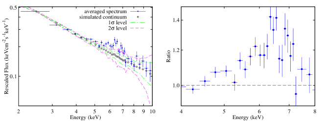
Figure 3: Left-hand panel: Stacked source spectrum (blue points with error bars), simulated power-law continuum (open circles), and its confidence ranges at the 1$\sigma$ (68 per cent) and 2$\sigma$ (90 per cent) levels for each energy bin, respectively. The green dot-dashed line and the red dashed line are the 1$\sigma$ and 2$\sigma$ levels for each bin, respectively. Right-hand panel: Ratio of the stacked source spectrum to the stacked simulated power-law continuum in the 4–8 keV range, resembling closely the characteristic relativistic broad Fe $\mathrm{K\alpha}$ line.

4 Modeling the broad line feature

We use Xspec  (version 12.8) to fit the stacked spectrum. The FTOOLS task flx2xsp is used to convert the flux spectrum into fits format which can be fitted using Xspec. Since we are interested in the broad emission feature, we use only the 3–8 keV band in the spectral fitting below. This avoids the somewhat large uncertainty in the higher energy band and the highly model-dependent unfolded spectrum (e.g., absorption, soft X-ray excess emission) below 3 keV (Corral et al., 2008). A simple power-law model leads to an unacceptable fit ($\mathrm{\chi^{2}/d.o.f}=156/22$), as expected, and other components have to be added. In the following fittings, we adopt the power-law fitted from the stacked simulated spectrum as the continuum model, with the slope and normalization parameters fixed at the best-fit values obtained above. In addition, a Gaussian component with the line energy fixed at 6.4 keV is also included to account for the unresolved narrow Fe $\mathrm{K\alpha}$ line which is ubiquitously found in AGN. We consider this model of the power-law plus the narrow Gaussian line as a baseline model. This baseline model only results a poor fit ($\mathrm{\chi^{2}/d.o.f}=106/25$), with an $EW\sim 114$ eV of the narrow line. Adding another Gaussian component with all the parameters free can improve the fit significantly ($\mathrm{\chi^{2}/d.o.f}=21/22$). This broad Gaussian component, with the line energy peaked at $\sim$6.2 keV and line width $\sim$0.8 keV, may indicate a broad line feature in the $\sim$5–7 keV energy range. Below we try to fit this broad profile using various models.

Table 2: Spectral fit in the 3.0-8.0 keV energy range

Baseline Model: Power-Law + Gaussian
Power-Law	Gaussian							$\chi^{2}/\rm{d.o.f}$
$\Gamma$	$E$(keV)	$\sigma~{}$(keV)	$EW~{}$(eV)
2.05(fixed)	6.4(fixed)	0.085c(fixed)	$\sim$114					106/25
Baseline⋆ + Partial Covering
Baseline			Pcfabs					$\chi^{2}/\rm{d.o.f}$
$\Gamma$	$EW_{6.4~{}\rm{keV}}$(eV)		$N_{\rm H}$a	covering factor
$\rm{2.31^{+0.27}_{-0.26}}$	$\rm{43\pm{25}}$		$\rm{44^{+20}_{-12}}$	$\rm{0.48^{+0.12}_{-0.15}}$				18/21
Baseline + LAOR + Emission Line(6.97 keV)/Absorption Line(6.67 keV)
Baseline		laor			Gaussian			$\chi^{2}/\rm{d.o.f}$
$\Gamma$	$EW_{6.4~{}\rm{keV}}$(eV)	$E$(keV)	$R_{\rm in}$	$EW~{}$(eV)	$E$(keV)	$\sigma~{}$(keV)	$EW~{}$(eV)
2.05(fixed)	$27^{+30}_{-27}$	$6.38^{+0.45}_{-0.08}$	$4.4^{+5.3}_{-1.7}~{}R_{\rm g}$	$\rm{362\pm 90}$	6.97(fixed)	0.085c(fixed)	$\rm{73\pm{30}}$	23/21
2.05(fixed)	$\rm{33\pm{27}}$	$6.75\pm{0.10}$	$3.7^{+1.8}_{-1.2}~{}R_{\rm g}$	$\rm{580\pm 120}$	6.67(fixed)	0.085c(fixed)	$20^{+22}_{-20}$	21/21
Baseline + RELLINE + Emission Line(6.97 keV)/Absoprtion Line(6.67 keV)
Baseline		relline			Gaussian			$\chi^{2}/\rm{d.o.f}$
$\Gamma$	$EW_{6.4~{}\rm{keV}}$(eV)	$E$(keV)	spin	$EW~{}$(eV)	$E$(keV)	$\sigma~{}$(keV)	$EW~{}$(eV)
2.05(fixed)	$21^{+30}_{-21}$	$6.34\pm 0.04$	$<0.66$	$\rm{364\pm 87}$	6.97(fixed)	0.085c(fixed)	$\rm{76\pm{30}}$	23/21
2.05(fixed)	$\rm{33\pm{27}}$	$6.73\pm 0.04$	$0.47^{+0.34}_{-0.39}$	$\rm{570\pm 120}$	6.67(fixed)	0.085c(fixed)	$21^{+22}_{-21}$	23/21
Baseline⋆ + RELLINE + Emission Line(6.97 keV)/Absorption Line(6.67 keV)
Baseline		relline			Gaussian			$\chi^{2}/\rm{d.o.f}$
$\Gamma$	$EW_{\rm{NL6.4~{}keV}}$(eV)	$E$(keV)	spin	$EW~{}$(eV)	$E$(keV)	$\sigma~{}$(keV)	$EW~{}$(eV)
$\rm{1.92\pm{0.08}}$	$13^{+39}_{-13}$	$6.33\pm{0.06}$	$<0.40^{b}$	$\rm{233\pm{113}}$	6.97(fixed)	0.085c(fixed)	$\rm{49\pm{32}}$	17/19
$\rm{1.92\pm{0.09}}$	$\rm{34\pm{27}}$	$6.71\pm{0.09}$	$<0.84^{b}$	$\rm{400\pm{227}}$	6.67(fixed)	0.085c(fixed)	$18^{+23}_{-18}$	18/19

$\star$: In this model, the photon index and normalization of the power-law are free parameters.

$a$: In unit of $10^{22}$ cm^-2.

$b$: $1\sigma$ confidence level.

$c$: This width corresponds to an unresolved narrow line in the ‘intrinsic’ spectra; see footnote 4 and Section 3.2

4.1 Relativistic broad line models

The broad feature around 6.4 keV observed in many Seyfert galaxies is widely believed to arise from the Fe $\mathrm{K\alpha}$ line emitted from the inner accretion disk close to the black hole, which is highly broadened and skewed due to relativistic effects and gravitational redshift. In this section we fit this feature in the stacked spectrum with such a relativistic line.

Laor model: We first adopt the laor model (Laor, 1991), which has been widely used in fitting relativistic Fe $\mathrm{K\alpha}$ lines in AGN. The laor model is fully relativistic, assuming the Kerr metric for a black hole with the maximum spin (dimensionless spin parameter $a=0.998$). The line energy, inner radius ($R_{\mathrm{in}}$) of the accretion disc and the normalization are free parameters, while the other parameters, which can not be well constrained, are fixed at their default values, e.g., the disc inclination $i=30$ degree and the emissivity index $q=3.0$. The laor model leads to a poor fit ($\mathrm{\chi^{2}/d.o.f}=41/22$) with the best-fit line energy at $\sim$6.39 keV. The large $\chi^{2}$ value results from a systematic structure in the residuals, which appears to be either an absorption due to Fe XXV (6.67keV) or an emission line identified as Fe XXVI (6.97keV). We consider these two scenarios respectively, by adding to the model an unresolved narrow Gaussian as an emission component (referred to as Case A hereafter) and as an absorption component (Case B); the line energies are fixed at the corresponding values and the line-widths are fixed at 85 eV (corresponding to an unresolved narrow line in the intrinsic spectrum; see footnote 4 and Section 3.2). As can be seen below, this improves the fitting significantly and results in acceptable fits (Table 2).

For Case A (narrow emission line of Fe XXVI), the best-fit line energy of the broad line component is $6.38^{+0.45}_{-0.08}$ keV with an $EW$ of $362\pm{90}$ eV. The best-fit inner radius of the disc is $R_{\mathrm{in}}=4.4^{+5.3}_{-1.7}~{}R_{\rm g}$. The $EW$s of the neutral narrow Fe $\mathrm{K\alpha}$ line and the high ionization narrow line components are 27 eV with an upper limit of 57 eV and $73\pm 30$eV, respectively. The fitted parameters are given in Table 2. Alternatively, for Case B (narrow absorption line of Fe XXV), the line energy of the broad component is $6.75\pm{0.10}$ keV, which may correspond to the K$\alpha$ transition of Fe XXV ions. The best-fit inner radius of the disc is $R_{\mathrm{in}}=3.7^{+1.8}_{-1.2}~{}R_{\rm g}$. The $EW$s of the broad component, the narrow Fe $\mathrm{K\alpha}$ component and the narrow absorption component are $580\pm{120}$ eV, $33\pm{27}$ eV and 20 eV with an upper limit of 42 eV, respectively.

Figure 4: Left-hand Panel: Spectral fit to the stacked spectrum with the best-fit model (dashed line), which comprises a power-law (with all parameters free) plus relline and a narrow emission line at 6.97 keV (Case A). The residuals as the data to model ratios are shown in the lower panel. Right-hand Panel: Broad Fe $\mathrm{K\alpha}$ complex of the stacked spectrum shown as the ratio of the data to the best-fit continuum (see text). The best-fit model (as in the left-hand panel; dot-dashed line) is shown for a comparison.

Figure 5: Same as Figure 4 except that the narrow line feature is fitted with an absorption line at 6.67 keV (Case B) instead of an emission line at 6.97 keV.

Relline model: A relativistic Fe $\mathrm{K\alpha}$ line with high S/N can be used to constrain the spin of the black hole, if the inner disc radius extends to the ISCO, which is a monotonic function of the spin parameter $a$. So far, black hole spins have been estimated in about two dozen AGN (e.g., Reynolds 2013, including the NLS1 1H0707-495), by using mostly the relativistic line models (e.g.,kerrdisk, Brenneman & Reynolds 2006; relline, Dauser et al. 2010). Here we assume that this method can also be applied to NLS1s, as did by others in previous work to estimate the black hole spin for a few individual NLS1s (Fabian et al., 2009; Marinucci et al., 2014)

We fit the broad-line component with relline model. The same as above, both Case A (with an unresolved 6.97 keV emission line) and Case B (with an unresolved 6.67 keV absorption line) are considered. Due to the relatively low S/N of the stacked spectrum, only the broad line energy and the spin of BH are free parameters. All the other parameters are fixed at default values (e.g., the emissivity index is fixed at 3.0 and the disk inclination fixed at 30 degree. Leaving the emissivity index free does not improve the fitting result and it can not be well constrained. When left as a free parameter, the best-fit inclination $i$ is $<10$ degree, which is somewhat small for Seyfert 1 galaxies. We thus fix it at 30 degree). In Case A, the relline model leads to an acceptable fit ($\mathrm{\chi^{2}/d.o.f}=23/21$). The broad line energy is $6.34\pm 0.04$ keV, corresponding to neutral Fe ions. The spin parameter is found to be $a<0.66$ (90 per cent significance level, see Figure 6, left panel) with a best-fit value of 0.10. The $EW$s of the broad line, narrow Fe $\mathrm{K\alpha}$ line and narrow high ionization line are similar to the laor model ($EW_{\rm BL}=364\pm 87$ eV, $EW_{\rm NL6.4~{}keV}=21$ eV with an upper limit of 51 eV and $EW_{\rm NL6.97~{}keV}=76\pm 30$ eV). In Case B, the model leads to an equally well fit ($\mathrm{\chi^{2}/d.o.f}=23/21$). The fitted energy of the broad line is $6.73\pm 0.04$ keV, implying that the line may originate from a highly ionized accretion disc. The $EW$s of the broad component, the narrow component and the absorption component are $570\pm 120$ eV, $33\pm 27$ eV and $21$ eV with an upper limit of 43 eV, respectively. The best-fit spin parameter is $0.47^{+0.34}_{-0.39}$ (90 per cent significance level, Figure  6, right panel). In either case, the inferred black hole spin from the composite Fe line profile is not very high.

The above fits are obtained by fixing the power-law index to that obtained from the stacked simulated power-law spectra. We also elevate this constraint by leaving the parameters of the power law component free in the fit. We find that, in both Case A and Case B, the best-fit photon index is slightly flatter than, but consistent within errors with, the simulated continuum, i.e., $1.92\pm 0.08$ for Case A and $1.92\pm 0.09$ for Case B. However, the BH spin can only be loosely constrained: in Case A $a<0.40$ and in Case B $a<0.84$ at the $68$ per cent confidence level. The equivalent width of the broad line is $233\pm 113$ eV and $400\pm{227}$ eV for Case A and Case B, respectively. The fitted parameters are shown in Table 2. The best-fit model for Case A and Case B are shown in Figures 4 and 5, respectively.

Blurred reflection model: As a more self-consistent approach, a reflection component, which is also likely subject to the relativistic effects, has to be considered. We model the spectrum with the baseline model plus a blurred reflection model as well as a narrow emission/absorption line. To implement this, we substitute the relline component with a smeared (cold) disc reflection component, i.e., pexmon$\ast$relconv (Dauser et al., 2010), in Case A. The spin, emissivity index, inclination angle and normalization are free parameters, while all the other parameters in the relconv component are fixed at default values, i.e., the inner radius of the accretion disc is fixed at the ISCO of the corresponding spin value; the outer radius is fixed at $400~{}R_{\mathrm{g}}$. The high-energy cut-off in the pexmon component is fixed at 1000 keV and the solar abundances are assumed. We obtain an excellent fit ($\mathrm{\chi^{2}/d.o.f}=17/18$) with the best-fit photon index of $2.08\pm{0.20}$ and the reflection fraction $R=1.3^{+1.7}_{-0.7}$. Both the inclination angle (the best-fit value $i=27$ degree) and the emissivity index (the best-fit value $q=3.3$) could not be well constrained and only lower limits are given, $i>22$ degree and $q>2.1$. An upper limit on the spin parameter $a<0.35$ (90 per cent confidence level) could be given if both the inclination and the emissivity index are fixed at their best-fit values.

The same procedure is applied to Case B but with an ionized reflection (i.e., pexriv plus a highly ionized emission line with the line energy of 6.67 keV and the line width of 1 eV) component. The disc temperature in pexriv is fixed at $10^{6}$ K and the inclination angle is fixed at 30 degree. The disc ionization cannot be constrained at all, and is thus fixed at $150~{}\mathrm{erg~{}cm~{}s^{-1}}$. Both the emissivity index and the reflection fraction parameters cannot be effectively constrained. We thus fix the emissivity index at a range of reasonable values, from 2.4 to 4.0 with a step of 0.2, and leave the reflection fraction as a free parameter. We find that this model can fit the stacked spectrum equally well for different emissivity indices ($\mathrm{\chi^{2}/d.o.f}\sim 17/18$). The best-fit reflection fraction $R$ is highly anti-correlated with the emissivity index. Both the fitted photon index (i.e., from $1.96$ to $2.31$ with a typical 90 per cent uncertainties of 0.35) and inclination (i.e., 24–29 degree with a typical 90 per cent uncertainties of 6 degree) remain consistent within their mutual uncertainties. The spin is constrained to be $a<0.8$ at the 90 (68) per cent confidence if the emissivity index is $>3.2$ ($<3.2$).

In conclusion, a detailed examination of the broad emission feature reveals a highly skewed broad line, which can be well fitted with relativistic line models of the Fe K$\alpha$. In addition, there is an indication for a possible narrow feature, either an emission (6.97 keV, Fe XXVI) or an absorption line (6.67 keV, Fe XXV) superimposing on the broad Fe line. The fitted energy of the relativistic line is consistent with neutral Fe in Case A, or with ionized Fe in Case B. In both cases, our analysis using the simple relativistic broad line model suggests low or intermediate values for the average spins of the black holes. A more self-consistent modeling incorporating relativistic reflection tends to be in accordance with these results, although the constraints on the spin values are of only low statistical significance. Future spectroscopic observations with higher S/N are needed to better constrain the black hole spin in these AGNs.

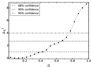
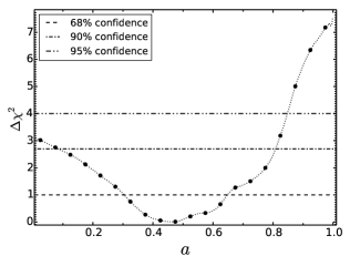
Figure 6: Error contour for the spin parameter, calculated using the relline model with the inclination angle fixed at 30 degree and the emissivity index fixed at 3.0, and the power-law slope is fixed at that obtained from the stacked simulated continuum. The three horizontal lines, from bottom to top, are corresponding to the 68 per cent, 90 per cent and 95 per cent confidence, respectively. Left-hand Panel: Case A (with a 6.97 keV narrow emission line); Right-hand Panel: Case B (with a 6.67 keV narrow absorption line).

4.2 Partial covering model

Although a broad line profile peaked at around 6.4 keV with a red wing can be explained by relativistic broad Fe $\mathrm{K\alpha}$ line which is likely to originated from the region close to the central black hole. The emergence of a broad profile may also be due to complex absorption (Miller et al., 2008). Gallo (2006) shown that some NLS1s exhibit spectral complexity in their X-ray spectra and can be explained either by disk reflection or partial covering (Tanaka et al., 2004, see also, e.g., Mrk 335, Gondoin et al. 2002; Longinotti et al. 2007; Grupe et al. 2008). We thus fit the stacked spectrum with the partial covering model (pcfabs in Xspec), leaving the photon index and normalization parameters of the power-law free. In this case, the partial covering model can fit the stacked spectrum well ($\mathrm{\chi^{2}/d.o.f}=18/21$) with column density $N_{\rm H}=4.4^{+2.0}_{-1.2}\times 10^{23}~{}\rm{cm}^{-2}$ and covering factor $\rm{CF}=0.48^{+0.12}_{-0.15}$. The best-fit photon index ($\Gamma=2.30\pm 0.28$) is somewhat larger than, but still marginally consistent with, the simulated continuum. The $EW$ of the narrow line is about $\sim 43\pm{25}$ eV. We also try to add an unresolved Gaussian emission line at 6.97 keV or absorption line at 6.67 keV to account for the potential emission or absorption line as shown in Figure 3. We find that adding an emission line at 6.97 keV does not improve the fit at all while the fitting result is slightly improved ($\mathrm{\chi^{2}/d.o.f}=17/20$) after adding an absorption line at 6.67 keV. The $EW$ of the 6.67 keV absorption line is about $\sim$11 eV (with an upper limit at $\sim$35 eV).

5 Discussion

By stacking the XMM-Newton spectra of a large sample of NLS1s, we find a significant broad line profile in the stacked spectrum, which appears to be elusive in the individual spectra. This broad line profile can be well explained with the relativistic broad line scenario. However, it’s also suggested that NLS1s show spectral complexity at X-ray energies (Gallo, 2006) and normally can be explained by either reflection from accretion disc or absorption by partial covering material along the line of sight. The broad line emerged in the stacked spectrum can also be fitted with partial covering model. Partial covering by neutral gas cannot be ruled out as an alternative explanation to the broad line-like feature shown in Figure 2. Some of the recent results from simultaneously XMM-Newton and NuSTAR observations seem to support the relativistic scenario (Risaliti et al., 2013; Marinucci et al., 2014), however. We thus take the interpretation of broad Fe line in this paper, and discuss the implications of our results in the context of this scenario. Our results thus suggest that the broad relativistic Fe $\mathrm{K\alpha}$ line is common in NLS1s, as in other Seyfert galaxies. The absence of broad Fe $\mathrm{K\alpha}$ line in most individual objects with high S/N in their X-ray spectra has been discussed in Nandra et al. (2007). In our sample this may be simply due to the relatively low spectral S/N around the Fe $\mathrm{K\alpha}$ line. This problem is perhaps also aggravated by the relatively steep continua of NLS1s on average, which means a small number of photon counts at high energies—thus poorly determined continuum spectra—and in the Fe $\mathrm{K\alpha}$ region.

5.1 Broad Fe line in NLS1s

Our results suggest that the fraction of broad relativistic Fe $\mathrm{K\alpha}$ line in NLS1s, which is still unclear (e.g., $\sim$13 per cent in the full sample of de La Calle Pérez et al. 2010 and 2 out of 4 in their flux limited sample), should not be low. We notice that the relativistic broad profiles are perhaps more common in low-luminosity ($L_{X}<1\times 10^{43}$ ergs s^-1, Guainazzi et al., 2006) AGN and in low-luminosity ($L_{X}<3\times 10^{44}$ ergs s^-1) or intermediate Eddington ratio ($\lambda\sim 0.1$) for high redshift Type 1 AGN (Iwasawa et al., 2012). Our results, with a median luminosity of $1.92\times 10^{43}$ ergs s^-1 and mean luminosity of $6.95\times 10^{43}$ ergs s^-1 in our sample, are in agreement with these previous work and may support the suggestion that relativistic broad profiles are more common in AGN with low-luminosities. Our results suggest that the broad Fe $\mathrm{K\alpha}$ line is perhaps also common in AGN with high Eddington ratio (e.g., NLS1s). This is consistent with the independence of the detectability of broad line on Eddington ratio (de La Calle Pérez et al., 2010).

The $EW$s of the broad line are $233\pm 113$ eV for Case A and $400\pm 227$ eV for Case B when fitted with relline models, leaving all the parameters in the power-law component free (see Table 2). Our results are consistent with what was found in de La Calle Pérez et al. (2010, an average $EW$ is of the order of 100 eV and less than 300 eV for individual source) for low-redshift AGN and is also in agreement with the results by Corral et al. (2008, an upper limit with 400 eV, fitted with the laor model). The best-fit energy of the broad line is around 6.7 keV in Case B, indicating a highly ionized accretion disc where the line originates from. A high ionization of thermal origin may be achieved by slim discs (Abramowicz et al., 1988). Alternatively, the high ionization of an accretion disc may also result from photoionization by hard X-ray radiation. As suggested in Ross & Fabian (1993), the effect of photoionization becomes important and may produce strong high ionization emission lines (e.g., Fe XXV emission lines) if the accretion rate exceeds 10 per cent of the Eddington rate. Considering the generally high accretion rates in NLS1s, the broad Fe $\mathrm{K\alpha}$ emission observed in the composite spectrum is more likely arising from highly ionized Fe ions, i.e., from highly ionized accretion discs, if the observed feature is indeed a 6.7 keV absorption line.

5.2 Neutral narrow Fe K$\alpha$ line in NLS1s

A neutral narrow Fe $\mathrm{K\alpha}$ line which may originate from cold material is ubiquitously found in nearby AGN. The $EW$ of the 6.4 keV narrow line is $<60$ eV, which is slightly weaker than the expected value (e.g., $\sim$60 eV) from the empirical Iwasawa-Taniguchi relation (IT relation, , Iwasawa & Taniguchi1993; Bianchi et al., 2007), but in agreement with that obtained by Zhou & Zhang (2010), in which shown that the $EW$ of neutral Fe $\mathrm{K\alpha}$ line in NLS1s is generally weaker than that from BLS1s. The relatively weaker 6.4 keV Fe $\mathrm{K\alpha}$ line may indicate a smaller covering factor of the reflecting matter which, as pointed out in Zhou & Zhang (2010), may be due to the high radiation pressure (Fabian et al., 2008) or outflows probably associated with the high Eddington ratio accretion in NLS1s (Komossa, 2008).

5.3 Ionized narrow Fe K$\alpha$ line in NLS1s

A narrow emission or absorption line is also suggested in the composite spectrum at energy around 6.7–7.0 keV, though the statistical significance is not very high. We tend to identify it as arising from highly ionized Fe ions, i.e., Fe XXVI in Case A or Fe XXV in Case B. High-ionization emission/absorption lines, of both low and high velocities, are often detected in the X-ray spectra of AGN (Bianchi et al., 2009; Fukazawa et al., 2011), and also in sources showing a relativistic broad Fe $\mathrm{K\alpha}$ line (, Miniutti et al.2007, e.g., MCG-6-30-15). For example, high-ionization, narrow Fe XXVI emission lines were detected in 21 out of 65 broad line Type 1 AGN and 12 out of 37 narrow line Type 1 AGN in Bianchi et al. (2009). Interestingly, high-ionization emission lines are also found in the stacked spectrum of a sample of AGN with high accretion rates selected from the XMM-COSMOS field (Iwasawa et al., 2012). It is thus not surprising to detect such emission/absorption lines in NLS1s.

In Case A, the $EW$ of the ionized line is $49\pm{32}$ eV which is in agreement with the result found in Fukazawa et al. (2011, 5-50 eV, Seyfert galaxies observed by Suzaku). We also notice that Iwasawa et al. (2012) found a significant highly ionized Fe K line in the XMM-COSMOS Type 1 sub-sample which includes sources with high Eddington ratios ($\log\lambda>0.6$). Considering that most NLS1s also have high accretion rate, this may indicate that there is a potential correlation between the high ionization Fe K emission line and the Eddignton ratio. Highly ionized Fe emission line can be produced via recombination and resonant scattering from ionized Compton-thin material far away from the central region, e.g., broad line region (BLR) or torus, as shown in Bianchi & Matt (2002). The observed $EW$ of $49\pm{32}$ eV, assuming a power law index of 2.0 and a solid angle of $0.26\times 4\pi$, can be produced from material with a column density larger than $\sim 10^{23}$ cm^-2 and an ionization parameter around $\log{U_{x}}\sim 0.2$.

In Case B, the absorption line is probably correspond to the Fe XXV resonant absorption line, likely produced in a Compton-thin photoionized material. The ionization parameter should be low (e.g., $\log{U_{x}}<0$, Bianchi et al. 2005) since no H-like iron absorption is detected in the stacked spectrum. The line $EW$ is $18^{+23}_{-18}$ eV, consistent well with Fukazawa et al. (2011, 5-40 eV), can be produced by material with column density larger than $10^{23}$ cm^-2.

In any case, an ionized Compton-thin material seems to be required to account for the potential high ionization emission/absorption feature in the stacked spectrum. We thus suggest that this kind of material should be ubiquitous in NLS1s and probably locates far from the central region, e.g., the BLR or torus.

5.4 Spin of the black holes in NLS1s

The black hole spin parameter constrained from the relativistic broad Fe K$\alpha$ line in the stacked spectrum is $a<0.66$ in Case A or $a<0.81$ in Case B using the relline model at the 90 per cent confidence level (the statistical significance is somewhat lower if the power-law continuum slope is set as a free parameter). A higher spin value is also unlikely to be the case using the blurred reflection model, though with a lower significance in some cases. This result indicates that the bulk of the black holes of NLS1s in the nearby universe (a median redshift $0.085$) either have averagely low or moderate spins, or distribute in a wide range of spins, from low spins to high ones; it is ruled out that most NLS1s have extremely large spins (e.g., $\ga 0.8-0.9$). This is the first time that the ensemble black hole spin parameters are constrained for NLS1s as a population. Note that a few individual NLS1s do have spin measurements with relatively small uncertainties from high S/N Fe K$\alpha$ line and X-ray reflection continuum, e.g., the spins of the black holes in two NLS1s, i.e., 1H0707-495 and SWIFT J2127.4+5654, are estimated to be $>0.89$ (Fabian et al., 2009) and $0.58^{+0.11}_{-0.17}$ (Marinucci et al., 2014), respectively. Interestingly, we note that the spin of J2127.5+5654 is consistent with the ensemble constraints obtained in this study.

NLS1s may represent an interesting and important phase in the growth and evolution of supermassive black holes (Komossa, 2008). Given their relatively small black hole masses and high accretion rates, there are suggestions that NLS1s are at an early stage of AGN evolution (Mathur, 2000). The distribution of the spins of the black holes may give insight into the processes of how their black holes grow and evolve. Theoretical models have shown that different processes of black hole growth lead to distinct distributions of the black holes spins. If black holes grow by merger only, the spin distribution would be bimodal with one peak at $a\sim$ 0.0 and the other at $a\sim$ 0.7. For processes of merger plus prolonged accretion, the overall spins are high ($a>0.9$). Low spins ($a<0.1$) will result from merger plus chaotic accretion processes (Berti & Volonteri, 2008). There have been suggestions that the evolution of NLS1s is driven by secular processes instead of major mergers, and their host galaxies possess mostly pseudo-bulges (Orban de Xivry et al., 2011, see also Mathur et al. 2012).

We first consider the prolonged accretion scenario by assuming an initial non-spinning black hole accreted continuously at the Eddington accretion rate with a radiation efficiency $\epsilon\sim 0.1$. Since prolonged accretion can spin up the black hole efficiently, the black hole will reach the maximum spin after an increase of its mass by a factor of $\sim 2.4$ only (King & Kolb, 1999). This takes roughly the Salpeter timescale ($\sim 5\times 10^{7}$yr, assuming the radiation efficiency $\epsilon\sim 0.1$) for AGN radiating at the Eddington luminosity. If the black hole spins turn out to be low or moderate, as is found in our work here, the AGN in NLS1s should be not only very young, much younger than $<5\times 10^{7}$ yr, but also with an initial spin close to 0. Given the relatively short time left for the black holes to grow, the current black hole masses of NLS1s would be on the same order of magnitude as the seed black holes, which would then be $\sim 10^{6}M_{\sun}-10^{7}M_{\sun}$. Since such high-mass seed black holes are not predicted by the current theories of black hole formation, the pure prolonged accretion scenario, in which black holes in NLS1s obtained their mass via continuous gas accretion onto initially much smaller seed black holes, seems to be inconsistent with our result.

Alternatively, the black holes in NLS1s may grow via mainly the process of chaotic accretion. Such a process would lead to low values of the final average spins, e.g., $a=0.1-0.3$ as found by King et al. (2008), which is in good agreement with what we found here ($a<0.66$ in the case where the narrow feature is an emission line). If confirmed, our result suggests that the growth and evolution of the black holes in the bulk of NLS1s are likely to proceed via the chaotic accretion process.

One should also note, however, the black hole spin parameter is constrained to be widely distributed ($a<0.81$) in the Case B (see Section 4.1). If this is true, then the chaotic accretion cannot be the main process to control the spin evolution of black holes in NLS1s provided that these black holes grow up from very small seeds. It is possible that the growth of each of these black holes is due to chaotic accretion with many episodes, in each episode the accretion is prolonged with a significant increase of black hole mass and significant spin evolution. In order to be compatible with a wide distribution of spin parameters among NLS1s, the black hole mass increase in each episode should be less than a factor of few.

To close this section, we note that the standard thin disk model is adopted in our study to fit the Fe K$\alpha$ line profile for NLS1s as common practice, however, which may be not valid for some NLS1s. Observations have suggested that some NLS1s may radiate at luminosities $\ga 30$ per cent of the Eddington luminosity, for which a slim disk model may be needed to describe the accretion (Abramowicz & Fragile, 2013). In the slim disk model, the disk is puffed up at the region close to the central black hole, the radiation from this region may be still efficient or may be not, and some radiation may be even emitted from the region within the innermost stable circular orbit (ISCO). Therefore, the Fe K$\alpha$ emission resulting from a slim disk model, if any, may be broader or less broad comparing with that expected from a thin disk model. In this case, it is not easy to directly relate the width and shape of the Fe K$\alpha$ line emission with the black hole spin due to the complications of the slim disk model.

6 Summary

In this paper, we study the ensemble property of the Fe $\mathrm{K\alpha}$ line in NLS1s by stacking the XMM-Newton spectra of a sample of 51 NLS1s observed in a total of 68 observations. By virtue of its highly improved S/N, the stacked spectrum reveals a prominent, broad emission feature, which can be well-fitted with relativistically broad line models, although a partial covering absorption model cannot be ruled out. Our result suggests that, as in Seyfert 1 galaxies, the relativistic Fe $\mathrm{K\alpha}$ line may in fact be common in NLS1s, which would be detected in the X-ray spectra of NLS1s with high S/N. The narrow 6.4 keV Fe $\mathrm{K\alpha}$ line is found to be much weaker than the expected value from the known Iwasawa-Taniguchi relation, which may indicate a smaller covering factor of the reflection material in NLS1s. The stacked spectrum also shows a possible high-ionization iron emission or absorption line, produced by ionised material far away from the central region. We also try to constrain the average spin of the black holes in NLS1s by modeling the stacked spectrum with relativistic line models. Our results tentatively suggest that the average spins are likely low or intermediate, and generally very fast spins ($\ga 0.8$) seem to be inconsistent with the data. This may favour the black hole growth scenario in NLS1s as chaotic accretion process or chaotic accretion with multi-episodes. Future high S/N, broad bandpass X-ray observations are needed to confirm these results.

References

- Abramowicz et al. (1988) Abramowicz M. A., Czerny B., Lasota J. P., Szuszkiewicz E., 1988, ApJ, 332, 646
- Abramowicz & Fragile (2013) Abramowicz M. A., & Fragile P. C., 2013, LRR, 16, 1
- Ai et al. (2011) Ai Y. L., Yuan W., Zhou H. Y., Wang T. G., Zhang S. H., 2011, ApJ, 727, 31
- Appenzeller et al. (1998) Appenzeller I., et al. 1998, ApJS, 117, 319
- Arnaud (1996) Arnaud K. A., 1996, in Jacoby G. H., Barnes J., eds, Astronomical Data Analysis Software and Systems V Vol. 101 of ASP Conf. Ser., p. 17
- Berti & Volonteri (2008) Berti E., Volonteri M., 2008, ApJ, 684, 822
- Bianchi et al. (2007) Bianchi S., Guainazzi M., Matt G., Fonseca Bonilla N., 2007, A&A, 467, L19
- Bianchi et al. (2009) Bianchi S., Guainazzi M., Matt G., Fonseca Bonilla N., Ponti G., 2009, A&A, 495, 421
- Bianchi & Matt (2002) Bianchi S., Matt G., 2002, A&A, 387, 76
- Bianchi et al. (2005) Bianchi S., Matt G., Nicastro F., Porquet D., Dubau J., 2005, MNRAS, 357, 599
- Boller et al. (1996) Boller T., Brandt W. N., Fink H., 1996, A&A, 305, 53
- Boroson (2002) Boroson T. A., 2002, ApJ, 565, 78
- Boroson & Green (1992) Boroson T. A., Green R. F., 1992, ApJS, 80, 109
- Brenneman & Reynolds (2006) Brenneman L. W., Reynolds C. S., 2006, ApJ, 652, 1028
- Caccianiga et al. (2004) Caccianiga A., et al. 2004, A&A, 416, 901
- Chaudhary et al. (2012) Chaudhary P., Brusa M., Hasinger G., Merloni A., Comastri A., Nandra K., 2012, A&A, 537, A6
- Corbin (1997) Corbin M. R., 1997, ApJS, 113, 245
- Corral et al. (2008) Corral A., et al. 2008, A&A, 492, 71
- Dauser et al. (2010) Dauser T., Wilms J., Reynolds C. S., Brenneman L. W., 2008, MNRAS, 409, 1534
- Denney et al. (2009) Denney K. D., Watson L. C., Peterson B. M., et al. 2009, ApJ, 702, 1353
- de La Calle Pérez et al. (2010) de La Calle Pérez I., et al. 2010, A&A, 524, A50
- Fabian et al. (2000) Fabian A. C., Iwasawa K., Reynolds C. S., Young A. J., 2000, PASP, 112, 1145
- Fabian et al. (1989) Fabian A. C., Rees M. J., Stella L., White N. E., 1989, MNRAS, 238, 729
- Fabian et al. (2008) Fabian A. C., Vasudevan R. V., Gandhi P., 2008, MNRAS, 385, L43
- Fabian et al. (2002) Fabian A. C., et al. 2002, MNRAS, 335, L1
- Fabian et al. (2009) Fabian A. C., et al. 2009, Nature, 459, 540
- Fukazawa et al. (2011) Fukazawa Y., Hiragi K., Mizuno M., Nishino S., Hayashi K., Yamasaki T., Shirai H., Takahashi H., Ohno M., 2011, ApJ, 727, 19
- Gallo (2006) Gallo L. C., 2006, MNRAS, 368, 479
- Gondoin et al. (2002) Gondoin P., Orr A., Lumb D., Santos-Lleo M., 2002, A&A, 388, 74
- Goodrich (1989) Goodrich R. W., 1989, ApJ, 342, 224
- Greene & Ho (2004) Greene J. E., Ho L. C., 2004, ApJ, 610, 722
- Greene & Ho (2007) Greene J. E., Ho L. C., 2007, ApJ, 670, 92
- Grupe (2004) Grupe D., 2004, AJ, 127, 1799
- Grupe et al. (1999) Grupe D., Beuermann K., Mannheim K., Thomas H.-C., 1999, A&A, 350, 805
- Grupe et al. (2008) Grupe D., Komossa S., Gallo L. C., Fabian A. C., Larsson J., Pradhan A. K., Xu D., Miniutti G., 2008, ApJ, 681, 982
- Grupe et al. (2004) Grupe D., Wills B. J., Leighly K. M., Meusinger H., 2004, AJ, 127, 156
- Grupe et al. (1998) Grupe D., Wills B. J., Wills D., Beuermann K., 1998, A&A, 333, 827
- Guainazzi et al. (2006) Guainazzi M., Bianchi S., Dovčiak M., 2006, Astronomische Nachrichten, 327, 1032
- Haddad & Vanderriest (1991) Haddad B., Vanderriest C., 1991, A&A, 245, 423
- Hornschemeier et al. (2005) Hornschemeier A. E., Heckman T. M., Ptak A. F., Tremonti C. A., Colbert E. J. M., 2005, AJ, 129, 86
- Iwasawa et al. (2012) Iwasawa K., et al. 2012, A&A, 537, A86
- (42) Iwasawa K. & Taniguchi Y., 1993, ApJ, 413, L15
- Kalberla et al. (2005) Kalberla P. M. W., Burton W. B., Hartmann D., Arnal E. M., Bajaja E., Morras R., Pöppel W. G. L., 2005, A&A, 440, 775
- King & Kolb (1999) King A. R., Kolb U., 1999, MNRAS, 305, 654
- King et al. (2008) King A. R., Pringle J. E., Hofmann J. A., 2008, MNRAS, 385, 1621
- Komossa (2008) Komossa S., 2008, in Rev. Mex. Astron. Astrofis. Conf. Ser. Vol. 32, p. 86
- Komossa & Xu (2007) Komossa S., Xu D., 2007, ApJL, 667, L33
- Laor (1991) Laor A., 1991, ApJ, 376, 90
- Leighly (1999) Leighly K. M., 1999, ApJS, 125, 317
- Longinotti et al. (2007) Longinotti A. L., Sim S. A., Nandra K., Cappi M., 2007, MNRAS, 374, 237
- Marinucci et al. (2014) Marinucci A., et al. 2014, MNRAS, 440, 2347
- Markowitz et al. (2006) Markowitz A., et al. 2006, Astronomische Nachrichten, 327, 1087
- Mathur (2000) Mathur S., 2000, MNRAS, 314, 17
- Mathur et al. (2012) Mathur S., Fields D., Peterson B. M., Grupe D., 2012, ApJ, 754, 146
- Miller (2007) Miller J. M., 2007, ARA&A, 45, 441
- Miller et al. (2008) Miller L., Turner T. J., Reeves J. N., 2008, A&A, 483, 437
- Mineshige et al. (2000) Mineshige S., Kawaguchi T., Takeuchi M., Hayashida K., 2000, PASJ, 52, 499
- (58) Miniutti G., et al. 2007, PASJ, 59, 315
- Miniutti et al. (2009) Miniutti G., Panessa F., de Rosa A., Fabian A. C., Malizia A., Molina M., Miller J. M., Vaughan S., 2009, MNRAS, 398, 255
- Moran et al. (1996) Moran E. C., Halpern J. P., Helfand D. J., 1996, ApJS, 106, 341
- Nandra et al. (1997) Nandra K., George I. M., Mushotzky R. F., Turner T. J., Yaqoob T., 1997, ApJ, 477, 602
- Nandra et al. (2007) Nandra K., O’Neill P. M., George I. M., Reeves J. N., 2007, MNRAS, 382, 194
- Nandra & Pounds (1994) Nandra K., Pounds K. A., 1994, MNRAS, 268, 405
- Orban de Xivry et al. (2011) Orban de Xivry G., Davies R., Schartmann M., Komossa S., Marconi A., Hicks E., Engel H., Tacconi L., 2011, MNRAS, 417, 2721
- Oshlack et al. (2001) Oshlack A. Y. K. N., Webster R. L., Whiting M. T., 2001, ApJ, 558, 578
- Osterbrock & Pogge (1985) Osterbrock D. E., Pogge R. W., 1985, ApJ, 297, 166
- Patrick et al. (2012) Patrick A. R., Reeves J. N., Porquet D., Markowitz A. G., Braito V., Lobban A. P., 2012, MNRAS, 426, 2522
- Peterson et al. (2004) Peterson B. M., Ferrarese L., Gilbert K. M., et al. 2004, ApJ, 613, 682
- Pounds et al. (1990) Pounds K. A., Nandra K., Stewart G. C., George I. M., Fabian A. C., 1990, Nature, 344, 132
- Puchnarewicz et al. (1992) Puchnarewicz E. M., et al. 1992, MNRAS, 256, 589
- Reynolds (2013) Reynolds C. S., 2013, Classical and Quantum Gravity, 24, 244004
- Risaliti et al. (2013) Risaliti G., Harrison F. A., Madsen K. K., et al. 2013, Nature, 494, 449
- Ross & Fabian (1993) Ross R. R., Fabian A. C., 1993, MNRAS, 261, 74
- Streblyanska et al. (2005) Streblyanska A., Hasinger G., Finoguenov A., Barcons X., Mateos S., Fabian A. C., 2005, A&A, 432, 395
- Tanaka et al. (2004) Tanaka Y., Boller T., Gallo L., Keil R., Ueda Y., 2004, PASJ, 56, L9
- Tanaka et al. (1995) Tanaka Y., et al. 1995, Nature, 375, 659
- Tatum et al. (2012) Tatum M. M., Turner T. J., Sim S. A., Miller L., Reeves J. N., Patrick A. R., Long K. S., 2012, ApJ, 752, 94
- Turner et al. (2002) Turner T. J., et al. 2002, ApJL, 574, L123
- Véron-Cetty & Véron (2006) Véron-Cetty M.-P., Véron P., 2006, A&A, 455, 773
- Véron-Cetty et al. (2001) Véron-Cetty M.-P., Véron P., Gonçalves A. C., 2001, A&A, 372, 730
- Wang et al. (1996) Wang T., Brinkmann W., Bergeron J., 1996, A&A, 309, 81
- (82) Watson M. G., et al. 2009, A&A, 493, 339
- Xu et al. (2003) Xu D. W., Komossa S., Wei J. Y., Qian Y., Zheng X. Z., 2003, ApJ, 590, 73
- Yaqoob & Padmanabhan (2004) Yaqoob T., Padmanabhan U., 2004, ApJ, 604, 63
- Zhou et al. (2006) Zhou H., Wang T., Yuan W., Lu H., Dong X., Wang J., Lu Y., 2006, ApJS, 166, 128
- Zhou & Wang (2005) Zhou X.-L., Wang J. M., 2005, ApJL, 618, L83
- Zhou & Zhang (2010) Zhou X.-L., Zhang S.-N., 2010, ApJL, 713, L11