Wigner’s quantum phase-space current in weakly-anharmonic
weakly-excited two-state systems

Abstract

There are no phase-space trajectories for anharmonic quantum systems, but Wigner’s phase-space representation of quantum mechanics features Wigner current $\bm{J}$. This current reveals fine details of quantum dynamics – finer than is ordinarily thought accessible according to quantum folklore invoking Heisenberg’s uncertainty principle. Here, we focus on the simplest, most intuitive, and analytically accessible aspects of $\bm{J}$. We investigate features of $\bm{J}$ for bound states of time-reversible, weakly-anharmonic one-dimensional quantum-mechanical systems which are weakly-excited. We establish that weakly-anharmonic potentials can be grouped into three distinct classes: hard, soft, and odd potentials. We stress connections between each other and the harmonic case. We show that their Wigner current fieldline patterns can be characterised by $\bm{J}$’s discrete stagnation points, how these arise and how a quantum system’s dynamics is constrained by the stagnation points’ topological charge conservation. We additionally show that quantum dynamics in phase space, in the case of vanishing Planck constant $\hbar$ or vanishing anharmonicity, does not pointwise converge to classical dynamics.

I Introduction

Classical phase-space trajectories allow the viewer to characterise a system’s dynamics at a glimpse. They also reveal rich structures such as the strange attractors of chaotic systems full of intricacies and beauty Berry (1978); Cvitanović et al. (2012).

Anharmonic quantum systems do not feature trajectories Oliva et al. , but fieldlines of Wigner’s phase-space current $\bm{J}$ characterise quantum-mechanical phase-space dynamics at a glimpse (Sections V and VI), similar to classical phase portraits: this is underexplored.

This is a gap this work aims to help fill.

Wigner’s quantum theory Wigner (1932) (Section II) is a representation of quantum mechanics in phase space Zachos (2002); Hirshfeld and Henselder (2002); Hancock et al. (2004); Rasinariu (2013); Zachos et al. (2005); Hillery et al. (1984); Case (2008); Kakofengitis et al. (2017) (additionally pioneered by Groenewold Groenewold (1946) and Moyal Moyal (1949)) equivalent to Heisenberg, Schrödinger and Feynman’s representations of quantum theory. It is, historically speaking, the third representation of quantum physics and its importance is still not clear: “Some believe it will supplant, or at least complement, the other methods in quantum mechanics and quantum field theory”Hirshfeld and Henselder (2002).

Here we investigate Wigner’s quantum phase-space current $\bm{J}$ and its fieldlines for the three classes of weakly-anharmonic potentials: hard, soft and odd potentials (Section IV). We emphasize the features the current patterns, associated with the three classes of potentials, have in common: it turns out that odd potentials are hybrids of hard and soft potentials and this is reflected in their phase-space current patterns (Sections V and VI).

We particularly stress an intuitive understanding of how the Wigner current patterns emerge (Subsections V.1 and V.2). Because the anharmonicities are weak, the $\bm{J}$-fieldline patterns can partly be understood from the vantage point of the harmonic oscillator (Section III) and partly through perturbation analyses (Sections VI.1 and V.3).

For simplicity, our discussions are limited to one-dimensional conservative quantum-mechanical systems featuring nearly harmonic potentials. We only consider the bound energy eigenstates (Section V) of weakly-excited systems in pure two-state superpositions (Section VI).

To demonstrate the conceptual power of the use of $\bm{J}$ and collections of its fieldlines, we show that in the limit of vanishing anharmonicity the fieldlines of $\bm{J}$ do not converge pointwise (Section V and VI) to those of the harmonic oscillator (Section III). This implies that in the limit of vanishing anharmonicity, or vanishing magnitude of Planck’s constant, quantum and classical phase-space behaviour are qualitatively very different from each other Oliva et al. ; Kakofengitis et al. (2017), see Sections V.2 and VII.

II Wigner distributions and Wigner current

We parameterize pure quantum two-state superpositions of energy eigenstates $\psi_{m}$ (with eigenenergies $E_{m}$ and energy difference $\Delta E=E_{n}-E_{m}$) by the mixing angle $\theta$

$$\Psi_{m,n}(x,t;\theta)=\cos(\theta)\psi_{m}(x)+\sin(\theta)e^{-\frac{i}{\hbar}\Delta Et}\psi_{n}(x)\;.$$ (1)

Here, $x$ and $t$ denote position and time, $\hbar=h/(2\pi)$ is Planck’s constant, and since this is a two-state superposition, the period time is

$$T_{m,n}=\frac{2\pi\hbar}{\Delta E}=\frac{2\pi\hbar}{|E_{n}-E_{m}|}\;.$$ (2)

Wigner’s phase-space quantum distribution $W(x,p,t)$ Wigner (1932); Hillery et al. (1984); Case (2008) is

$$W(x,p,t)\equiv\frac{1}{\pi\hbar}\int dy\,\varrho(x-y,x+y,t)e^{\frac{2i}{\hbar}py}\;;$$ (3)

where $\varrho(x-y,x+y,t)=\Psi(x-y)\Psi^{*}(x+y)$, for pure states. $W$ is real-valued, non-local (through $y$), and

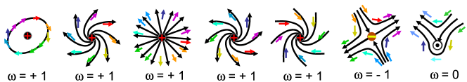
Figure 1: Wigner current stagnation points are characterised by their integer orientation winding number (7). A red plus sign labels stagnation points with topological charge Dennis et al. (2009) $\omega=+1$, a yellow minus sign $\omega=-1$, and a white circle $\omega=0$. The current’s fieldlines can be skewed near stagnation points in phase-space, can feature skewed separatrices, and saddles oriented in the $p$-direction.

normalized $\int\int dx\;dp\;W(x,p,t)=1$ (we abbreviate $\int=\int_{-\infty}^{\infty}$).

Wigner’s distribution $W$ is set apart from other quantum phase-space distributions Hillery et al. (1984) by the fact that only $W$ simultaneously yields the correct projections in position and momentum ($\varrho(x,x,t)=\int dp\;W$ and $\tilde{\varrho}(p,p,t)=\int dx\;W$) as well as state overlaps $|\langle\psi_{1}|\psi_{2}\rangle|^{2}=2\pi\hbar\int\int dx\;dp\;W_{1}\;W_{2}$, while maintaining its form (3) when evolved in time. Additionally, the Wigner distribution’s averages and uncertainties evolve momentarily classically Royer (1992); Ballentine et al. (1994) (fulfilling Ehrenfest’s theorem Kakofengitis et al. (2017)). This is why $W$ is the “closest quantum analogue of the classical phase-space distribution” Zurek (2001).

To study $W$’s dynamics one Wigner-transforms von Neumann equation $\partial_{t}\varrho=-\frac{i}{\hbar}[H,\varrho]$, analogously to Eq. (3). The result can be cast into the form of Wigner’s continuity equation Wigner (1932)

$$\partial_{t}W+\partial_{x}J_{x}+\partial_{p}J_{p}=0\;,$$ (4)

here $\bm{J}(x,p,t)$ denotes the Wigner current Steuernagel et al. (2013) and the shortened notation $\frac{\partial^{2}}{\partial x^{2}}=\partial_{x}^{2}$, etc., is used for partial derivatives.

In the case of potentials that can be Taylor-expanded, $\bm{J}$ assumes the infinite-sum form Wigner (1932); Groenewold (1946); Moyal (1949); Donoso and Martens (2001); Schleich (2001); Case (2008); Bauke and Itzhak

$$\bm{J}=\begin{pmatrix}J_{x}\\ J_{p}\end{pmatrix}=\begin{pmatrix}\frac{p}{M}W\\ -\sum\limits_{l=0}^{\infty}{\frac{(i\hbar/2)^{2l}}{(2l+1)!}\partial_{p}^{2l}W\partial_{x}^{2l+1}V(x)}\end{pmatrix}\;,$$ (5)

where $M$ is the mass of the particle. The term $J_{p,l=0}$ is of classical form, the terms of higher order in $l$ are known as quantum correction terms.

In general $J_{p}$ in (5) has the integral form Wigner (1932); Kakofengitis et al. (2017)

$$J_{p}=-\frac{1}{\pi\hbar}\int dy\;\left[\frac{V(x+y)-V(x-y)}{2y}\right]\\ \times\varrho(x-y,x+y,t)e^{\frac{2i}{\hbar}py}\;.$$ (6)

For numerical stability we avoid the infinite-sum form of $J_{p}$ in (5), when generating the $\bm{J}$’s fieldlines depicted in Figs. 5, 7, 8 and 10, and use its integral form (6) instead.

II.1 Stagnation points of quantum phase-space current

Wigner current reveals detail of quantum dynamics’ finest features, in particular the nature of its stagnation points, the points in phase-space where the dynamics momentarily stops. In classical physics, stagnation points are also referred to as equilibrium, stationary, fixed, critical, invariant and rest points Cvitanović et al. (2012). This multitude of terms testifies to their central importance in classical mechanics as well as wave theory, e. g. in the field of ‘singular’ optics Dennis et al. (2009) (where they are called singular points Berry (2000)).

In classical physics stagnation points can only form on the $x$-axis at the potential’s minima, maxima and saddle points, where the force is zero.

In quantum physics Wigner distributions are known to feature negative regions in phase-space Wigner (1932). In these regions the current is inverted in direction Steuernagel et al. (2013), this leads to the formation of whorls and saddle flows with points of stagnating current at their centers. This can happen wherever in phase-space the Wigner distribution turns negative.

Analogously to the classical case, Wigner current’s stagnation points are the most important points in quantum phase-space for two reasons: the topological nature of Wigner current’s stagnation points, firstly, orders the current in large surrounding sectors of phase-space and, secondly, makes them carry a conserved topological charge. Its topological nature makes their appearance robust to perturbations and time evolution.

To quantify the topological charge conservation of $\bm{J}$’s stagnation points, we use the orientation winding number for Wigner current along closed, self-avoiding loops $\cal L$ in phase-space Steuernagel et al. (2013)

$$\omega({\cal L},t)=\frac{1}{2\pi}\varointctrclockwise_{\cal L}d\varphi\;;$$ (7)

where $\varphi$ is the angle between $\bm{J}$ and the $x$-axis, see fig. 1. Since the components of the current are continuous functions, $\omega$ is zero except for the case when the loop $\cal L$ contains stagnation points, such as those sketched in fig. 1. Then, a non-zero value of $\omega$ can occur. The value of $\omega$, (in mathematics known as the stagnation point’s Poincaré-Hopf index), is topologically protected Dennis et al. (2009). When the system’s dynamics transports a stagnation point across $\cal L$, $\omega({\cal L},t)$ can change Steuernagel et al. (2013). The topological charges can be combined or split through the system’s time evolution while their sum remains conserved Steuernagel et al. (2013).

III Wigner current of Harmonic Oscillators

Figure 2: Top row: Wigner current and Wigner distributions for the harmonic oscillator potential (8). Bottom row: Fieldlines of the integrated Wigner current $\bm{J}(x,p,t)$ at fixed time $t$. Left column: first excited state $\psi_{1}$. Right column: the superposition $\Psi^{\odot}_{0,1}(\frac{7T}{8};\frac{\pi}{3})$. Dashed black circles show the locations of $W=0$ which implies that, because of Eq. (9), $J^{\odot}_{x}=0$ (thick green lines) and $J^{\odot}_{p}=0$ (thick blue lines). These dashed black lines constitute circular current stagnation lines with constant radius $R^{\odot}_{1}=1/\sqrt{2}$ and a centre which is further displaced from the origin (10) the smaller the mixing angle $\theta$ in (1). In the top row the background coloring refers to the respective Wigner distributions’ values (compare insets). The normalised Wigner current $\bm{J}/|\bm{J}|$ is depicted with red arrows if the Wigner distribution is positive. For negative Wigner distribution green arrows are used, demonstrating current reversal Steuernagel et al. (2013). White arrows on top of $\bm{J}/|\bm{J}|$ depict the magnitude of $\bm{J}$. Bottom row: The depicted Wigner current fieldlines run through randomly picked points. The stagnation point at the origin carries topological charge $\omega=+1$ and is labelled as in fig. 1.

When we introduce weakly-anharmonic potentials in section IV, we rescale them to match their minimum’s curvature to our choice of a harmonic reference potential

$$V^{\odot}(x)=\frac{x^{2}}{2}\;,$$ (8)

with circular fieldlines (rather than elliptical Peder Dahl and Springborg (1988)), see fig. 2. Having such circular fieldlines is the main motivation for this particular choice. It constitutes a choice of units of mass $M=1$, spring constant $k=1$. Setting $\hbar=1$, leads to an angular frequency of $\Omega^{\odot}=1$ and an oscillation period of $T^{\odot}={2\pi}$.

Wigner current for $V^{\odot}$, according to Eq. (5), has the ‘classical’ form (see Takabayasi Takabayasi (1954) p.351)

$${\bm{J}}^{\odot}=W^{\odot}(x,p,t)\cdot\binom{p}{-x}\,.$$ (9)

III.1 Degenerate Wigner current

Wigner distributions are continuous and have negativities Wigner (1932), they therefore feature zero-contours in phase-space which, in the case of the harmonic oscillator, because of the form (9) of $\bm{J}$, become zero-lines for both components, $J^{\odot}_{x}$ and $J^{\odot}_{p}$ simultaneously, giving rise to lines of stagnation of the current, see fig. 2.

It is well known from quantum optics that the eigenstates $W^{\odot}_{n,n}(x,p)$ of the harmonic oscillator Fock states $\psi_{n}^{\odot}$ resemble Mexican hats centred on the origin, with concentric fringes of alternating polarity. Their zero-contours thus form concentric circles Schleich (2001).

In the case of superposition states, we primarily investigate superpositions of ground and first excited state $\Psi_{0,1}(t;\theta)$ (1), in which case $W$’s circular zero-contour remains a circle with constant radius $R^{\odot}_{1}=1/\sqrt{2}$ but shifted centre position $C_{01}$. The centre is further displaced from the origin the larger the groundstate contribution ($\theta\downarrow 0$ in $\Psi_{0,1}(\theta)$ (1)) and rotates around the origin, with frequency $\Omega^{\odot}=1$, according to

$$C_{0,1}(t;\theta)=\left(-R^{\odot}_{1}\cos(t)\cot(\theta),R^{\odot}_{1}\sin(t)\cot(\theta)\right)\;,$$ (10)

compare Figs. 2 and 9.

IV The Three Classes of Weakly-Anharmonic Potentials

Weakly-anharmonic potentials $V(x)$ that admit a Taylor expansion in $x$ are characterized by their leading anharmonic term $\alpha_{\nu}x^{\nu}$ in what we will refer to as their truncation $V^{\cal A}_{\nu}$ of order $\nu$, and representative $\cal A$, namely,

$$V^{\cal A}(x)\approx V^{\cal A}_{\nu}(x)=\frac{x^{2}}{2}+\alpha_{\nu}^{\cal A}x^{\nu}=V^{\odot}(x)+\alpha_{\nu}^{\cal A}x^{\nu}\,.$$ (11)

Potential	Harmonic Oscillator	Eckart (hard)	Rosen-Morse (soft)	Morse (odd)
$V^{\cal A}(x)$	$V^{\odot}=\frac{x^{2}}{2}$	$V^{\cal E}=D\tan^{2}\left(\frac{x}{\sqrt{2D}}\right)$	$V^{\cal R}=D\tanh^{2}\left(\frac{x}{\sqrt{2D}}\right)$	$V^{\cal M}=D\left(1-e^{-\frac{x}{\sqrt{2D}}}\right)^{2}$
$V_{\nu}^{\cal A}=\frac{x^{2}}{2}+\alpha_{\nu}^{\cal A}x^{\nu}$	$V^{\odot}=\frac{x^{2}}{2}$	$V_{4}^{\cal E}=\frac{x^{2}}{2}+\frac{x^{4}}{6D}$	$V_{4}^{\cal R}=\frac{x^{2}}{2}-\frac{x^{4}}{6D}$	$V_{3}^{\cal M}=\frac{x^{2}}{2}-\frac{x^{3}}{2\sqrt{2D}}$
Eigenvalues	$n+\frac{1}{2}$	$D\left[\left(\frac{\sqrt{1+16D^{2}}+2n+1}{4D}\right)^{2}-1\right]$	$D\left[1-\left(\frac{\sqrt{1+16D^{2}}-2n-1}{4D}\right)^{2}\right]$	$D\left[1-\left(\frac{4D-2n-1}{4D}\right)^{2}\right]$
$\mbox{Groundstate\quad}\atop\mbox{(unnormalized)}$	$e^{-\frac{x^{2}}{2}}$	$\cos\left(\frac{x}{\sqrt{2D}}\right)^{\left[\frac{\sqrt{1+16D^{2}}+1}{2}\right]}$	${\rm sech}\left(\frac{x}{\sqrt{2D}}\right)^{\left[\frac{\sqrt{1+16D^{2}}-1}{2}\right]}$	$e^{-\left[x\left(\frac{4D-1}{2\sqrt{2D}}\right)+2De^{-\frac{x}{\sqrt{2D}}}\right]}$
$D$-parameter	-	$D>0$	$D>\sqrt{\left(\frac{2N-1}{4}\right)^{2}-\frac{1}{16}}$	$D>\frac{2N-1}{4}$
$N$ bound states	-	-	$N(D)=\left\lfloor\frac{\sqrt{1+16D^{2}}+1}{2}\right\rfloor$	$N(D)=\left\lfloor\frac{4D+1}{2}\right\rfloor$

Table 1: The quantum harmonic oscillator and the three classes of anharmonic potentials are presented together with their corresponding energy eigenvalues and groundstate Dutt et al. (1988) ($n=0,1,2,\ldots,N-1$). The inverse anharmonicity parameter $D$ ($\lim_{D\rightarrow\infty}V^{\cal E,R,M}=V^{\odot}$) is also the depth of the two open potentials ($V^{\cal R}$ and $V^{\cal M}$). The last row gives the number of bound states $N$ in terms of $D$, where $\left\lfloor\ldots\right\rfloor$ denotes floor rounding. Higher excited energy eigenstates are easily created from the groundstates using SUSY-QM techniques Dutt et al. (1988).

The precise order $\nu$ of a truncation’s leading anharmonic term $\alpha_{\nu}^{\cal A}x^{\nu}$ is quite unimportant for our discussion, as it is the qualitative class of the potential that determines its qualitative dynamic features we are primarily interested in.

With respect to qualitative features of Wigner current for weakly-excited bound state systems, just as for the associated phase portraits in the classical case, see fig. 3, only three classes of anharmonic potentials exist: hard, soft, and odd potentials. We checked this numerically for several potentials and it is plausible from our discussion below.

All potentials with a leading positive anharmonic term of even order have qualitatively similar classical phase-space profiles. They correspond to springs harder than their Hookian reference (8), see left column of fig. 3. Soft potentials have a negative leading term of even order, fig. 3, middle column. For potentials of a leading term of odd order we always set the leading term $\alpha_{\nu}<0$, making the odd potentials soft for $x>0$ and hard for $x<0$, fig. 3, right column.

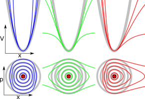
Figure 3: Top row: Representatives of the three classes of weakly anharmonic potentials displayed side by side: Eckart potentials ($V^{\cal E}$, left, in blue) are hard, Rosen-Morse potentials ($V^{\cal R}$, centre, in green) are soft and Morse potentials ($V^{\cal M}$, right, in red) are odd, see Table 1. The potentials feature differing amounts of anharmonicity, $\alpha_{\nu}^{\cal A}$ (11), while all are rescaled to have the same minimum curvature as the harmonic reference potential $V^{\odot}$ (8) (displayed behind each class as a thick grey line).
Bottom row: energy contours (for one fixed potential strength in each column) superimposed on harmonic oscillator’s circular energy contours (thick grey lines).

For each class a representative exists for which all bound state eigenfunctions and eigenenergies are known in simple closed form Dutt et al. (1988). As such representatives we choose the hard Eckart, $V^{\cal E}$, soft Rosen-Morse, $V^{\cal R}$, and odd Morse potential, $V^{\cal M}$; see fig. 3 and Table 1. For the Morse case all bound-state Wigner distributions are known Peder Dahl and Springborg (1988) and were used to cross-check some of our numerical calculations.

Anharmonic potentials $V^{\cal A}$ which, based on their truncation $V^{\cal A}_{\nu}$, are classed as even or odd can contain higher order Taylor terms which are not necessarily only even or odd. The influence of such higher terms can be neglected since we limit our investigation to weakly excited systems. If we were to regard the truncated right hand side of Eq. (11) as the full potential, soft and odd potentials would obviously have no bound eigenstates; we exclude such cases.

With these provisions, studying one representative of each class allows us to cover qualitative features of Wigner current of the bound states of all weakly-excited weakly-anharmonic potentials.

V Wigner current patterns for Eigenstates of anharmonic potentials

The degeneracy of Eq. (9) leads to formation of lines of stagnation Steuernagel et al. (2013) in the harmonic case. When anharmonicities are ‘turned on’ ($\alpha_{\nu}>0$), the zero-lines of the respective current components $J_{x}$ and $J_{p}$ get shifted by different amounts. This results in the formation of stagnation points in phase-space where the two components’ zero-lines cross; compare fig. 2 with 4 and 5 where thick green lines show where $J_{x}=0$ and thick blue lines where $J_{p}=0$.

An intuitive understanding of the ensuing Wigner current patterns is discussed next.

V.1 Existence of distinct Stagnation Points of Wigner Current

The anharmonicity of the potential deforms the zero-contours of $W$ shifting the zero-lines of the $J_{x}$-component ($J_{x}=\frac{p}{M}W$). The $J_{p}$-zero-lines get shifted differently due to the additional presence of the quantum corrections terms in Eq. (5): anharmonic quantum-mechanical systems form discrete current stagnation points in phase-space whenever $\hbar>0$.

Figure 4: Qualitative discussion of emergence of type and positioning of Wigner current stagnation points for first excited state of a hard potential. White arrows represent normalized Wigner current as observed in the harmonic case; clockwise, far from the origin and, anti-clockwise (inverted current), very close to the origin (compare left panels of fig. 2). Green and blue ellipses represent the zero-circles, see Section III.1, deformed by the anharmonicity of the potential. They are colored green when $J_{x}$ changes sign and blue when $J_{p}$ does, this also applies to $x$ and $p$-axis. To ‘fill the plane’ we track the orientation of the current while moving across phase-space along the sequence of arrows with ever darker shades of grey which eventually wraps around the rightmost ‘+1’-stagnation point. Whenever this sequence crosses a zero-line, when $J_{x}=0$ or $J_{p}=0$, the arrows are framed green or blue, respectively. We can, similarly, track the current’s orientation around the boundaries of the deformed zero-circles and along $x$ and $p$-axis. Green arrows with blue fringe are orientated horizontally ($J_{p}=0$) and invert direction whenever the blue line they are pinned to crosses a green line. Blue arrows with green fringe are tied to green lines, are vertically aligned, and behave analogously. At every crossing of a green with a blue line a stagnation point exists, but nowhere else. Having ‘filled the plane’ we can work out the topological charge of the stagnation points, labelled as the symbols of fig. 1. The quantitative plots in the top row of fig. 5 confirm this qualitative analysis.

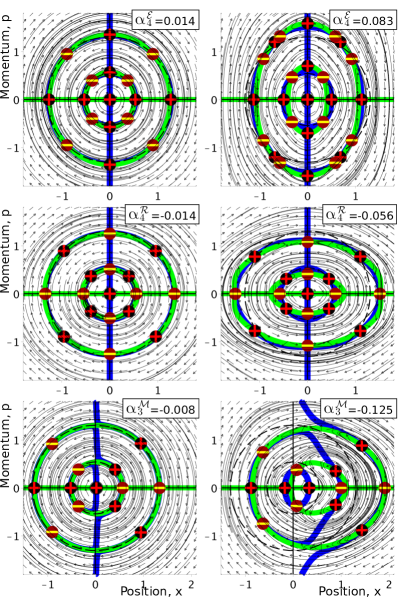
Figure 5: Wigner current patterns of the first excited state (left frame) and second excited state (right frame) for the three classes of weakly-anharmonic potentials: top row, (hard) Eckart, middle row, (soft) Rosen-Morse, bottom row, (odd) Morse. Note that the current patterns of odd potentials feature shapes of the hard case (for $x<0$) and the soft case (for $x>0$). The anharmonicity $\alpha_{\nu}^{\cal A}$ in Eq. (11) increases from left to right, with the respective values quoted in each panel, corresponding to values of $D=$ (12, 2) (top row), (12, 3) (middle row), and (2048, 8) (bottom row). Symbols, linestyles and their coloring have been adopted from fig. 2 (dashed black lines show zeros of $W^{\odot}$). The stagnation points at the thick zero-lines’ crossings are labelled as in fig. 1. All fieldlines form closed loops, $\bm{\nabla}\cdot\bm{J}=0$, since for eigenstates $\partial_{t}W=0$.

In short, weakly-anharmonic systems are fundamentally non-classical Oliva et al. ; Kakofengitis et al. (2017). The Wigner distributions for energy eigenfunctions of a weakly-anharmonic system converge pointwise towards those of the harmonic oscillator, but $\bm{J}$ and its fieldlines do not. In this sense there cannot be a smooth transition from quantum to classical case in either the limit of $\hbar\rightarrow 0$ or vanishing non-linearity in the potential.

This is at variance with published statement such as — “Trajectory methods […] are not reliable in general, being restricted to interaction potentials which do not deviate too much from an harmonic potential.” Daligault (2003), or: “the first step toward a systematic and general Wigner description is to consider a system whose potential differs only slightly from a harmonic potential” Lee and Scully (1982).

Instead, we find that very weakly anharmonic quantum systems develop quantum coherences essentially just like more strongly anharmonic systems, only more slowly.

V.2 Qualitative Effects of Anharmonicities: features of eigenstates’ current stagnation points

Heisenberg’s uncertainty principle $\Delta x\cdot\Delta p\geq\hbar/2$ implies constancy of the size of an uncertainty domain in phase-space Walls and Milburn (1994) (note that this argument must not be taken too far Zurek (2001)). Hard potentials squash phase-space fieldlines in position thus elliptically expanding them in momentum, see bottom row of fig. 3. This observation can be applied to the shape of $W$’s zero-circles (Section III.1) as well: compare the green lines in fig. 4 and in the top row of fig. 5. Soft potentials invert this scenario, expansion in $x$ leads to an elliptical squeeze in $p$, see middle row of fig. 5. Odd potentials are effectively hard on the left and soft on the right side. This leads to a growth in position spread and reduction in momentum spread, similar to the case of soft potentials; but, additionally, phase-space features tend to be moved to the right, towards the side where the potential is open, see bottom row of fig. 5 and our discussion on the displacement of the minimum vortex in section VI.1.

The $x$-axis is colored green to mark the vanishing of the component $J_{x}$, yielding two stagnation points for all (blue) $J_{p}$-zero-circles intersecting it. Similarly, the $p$-axis is a blue line in the harmonic case, and, for symmetry reasons, also for even potentials. For odd potentials these $J_{p}$ zeros do not lie on the $p$-axis but are displaced to the right, see bottom row in fig. 5.

In section V.3 we confirm these statements through a mathematical analysis.

Can an alternative to the break-up of the $J_{p}$ zero-lines for odd potentials, see bottom row of fig. 5, exist?

The answer is –it cannot: to the left of the $p$-axis an odd potential is hard and therefore has to yield the characteristic pattern displayed in the top row of fig. 5, to the right it is soft, yielding the middle row pattern. Near the $p$-axis both patterns meet but cannot be connected due to the continuity of $J_{x}$ and $J_{p}$ as functions of $x$ and $p$. The only option, respecting continuity, is the cut-and-reconnect pattern we see realised in bottom row of fig. 5.

In the limit of vanishing anharmonicity, four stagnation points form on the diagonals $|x|=|p|$ per zero-circle. These positions can be understood from the above observations. The elliptic squashing and expansion of the zero-circles of $J_{x}$ and $J_{p}$ is weak, leading to deformation of a zero-circle into two ellipses with small, slightly different eccentricities, common centres and equal area which are aligned with the coordinate axes of phase-space. In the limit of vanishing eccentricities these intersect at odd multiples of 45 degrees forming the diagonal stagnation points we observe in Figs. 4 and 5.

To summarize this qualitative discussion:

Weakly-anharmonic even potentials have $8n+1$ stagnation points for all low lying eigenstates $\psi_{n}$: one near the origin, 4 diagonal stagnation points and 4 stagnation points: 2, where the $J_{p}$-zero-lines cross the $x$-axis, and 2, where the $J_{x}$-zero-lines cross the $p$-axis.

Weakly-anharmonic odd potentials have $6n+1$ stagnation points per eigenstate, since the $p$-axis stagnation points are avoided by the cut-and-reconnect mechanism, mentioned above.

For very great anharmonicities some of our results are approximations, see top right-most panel of fig. 5.

V.3 For eigenstates, displacement of $J_{p}=0$, on the $x$-axis, is less than that of $J_{x}=0$

Numerically, we see that the zero lines of $J_{x}$ and $J_{p}$ shift differently. We now confirm analytically our qualitative discussion in section V.2.

For the displacement analysis of weakly anharmonic potentials we use $\bm{J}$ up to first order in $l$, in Eq. (5). Because $\alpha_{\nu}\ll 1$, $W\approx W^{\odot}$ and $J_{x}\approx pW^{\odot}$. Furthermore

$$J_{p} \approx-W^{\odot}\partial_{x}V_{\nu}+\frac{\hbar^{2}}{24}\partial^{2}_{p}W^{\odot}\partial^{3}_{x}V_{\nu}$$ (12)

$$=-xW^{\odot}+\frac{\hbar^{2}\nu!}{24(\nu-3)!}\cdot\alpha_{\nu}x^{\nu-3}\cdot\partial^{2}_{p}W^{\odot}\;,$$ (13)

and $$\partial_{x}J_{p}\approx\partial_{x}\left(-W^{\odot}\partial_{x}V_{\nu}\right)=-W^{\odot}-x\partial_{x}W^{\odot}\;.$$ (14)

We determine the displacement $\delta x_{J_{p}}$ of the zeros of $J_{p}$ on the $x$-axis using the Newton gradient method at $(x,p)=(\tilde{X},0)$, here $\tilde{X}$ denotes the point where the Wigner distribution is zero, i.e., where $J_{x}=0$. Thus, $\delta x_{J_{p}}|_{(\tilde{X},0)}\approx-J_{p}|_{(\tilde{X},0)}/\partial_{x}J_{p}|_{(\tilde{X},0)}$, which yields

$$\Big{.}\delta x_{J_{p}}\Big{|}_{(\tilde{X},0)}\!\!\approx\left.\frac{\hbar^{2}\nu!}{24(\nu-3)!}\cdot\alpha_{\nu}x^{\nu-4}\cdot\frac{\partial^{2}_{p}W^{\odot}}{\partial_{x}W^{\odot}}\right|_{(\tilde{X},0)}\!\!.$$ (15)

Now, the Mexican hat profiles of the harmonic oscillator’s Wigner distributions (see insets fig. 2) imply that $\partial^{2}_{p}W_{n,n}^{\odot}/\partial_{x}W_{n,n}^{\odot}|_{(\tilde{X},0)}$ is positive for $\tilde{X}>0$ and negative for $\tilde{X}<0$.

For example, if the potential is stiff and symmetric ($\alpha_{4}>0$) we know that the contours of $W$ are squeezed inward on the $x$-axis, due to the uncertainty principle. In other words the magnitude of the zeros of the Wigner distributions on the $x$-axis obey $|\tilde{X}_{W}|<|\tilde{X}_{W^{\odot}}|$. In this case $\Big{.}\delta x_{J_{p}}\Big{|}_{(\tilde{X},0)}>0$, which counteracts the inward movement of the zeros of $J_{x}$; the zero line of $J_{p}$ is less deformed than that of $J_{x}$.

The same logic can be applied to soft weakly-anharmonic potentials. Although for odd potentials a higher order in $l$ of Eq. (5) has to be used, this discussion confirms that an odd potential’s behaviour constitutes a hybrid of stiff and soft potentials’ behaviour, see subsection V.2 and fig. 5.

Additionally, the discussion above shows that quantum dynamics in phase space, in the case of vanishing Planck constant $\hbar$ or vanishing anharmonicity, does not pointwise converge to classical dynamics.

VI Wigner current patterns for Two-State Superpositions

We now consider superpositions of energy eigenstates. Note that the associated fieldline patterns presented in Figs. 7, 8 and 10, are integrated lines of $\bm{J}$ at one moment in time only. They therefore do not represent the time-evolution of $\bm{J}$, but an illustrative, albeit somewhat unphysical, momentary snapshot.

VI.1 Displacement of the minimum vortex

Similarly to Eq. (15), with the Newton gradient method we we determine the $x$-shift of the zero of $J_{p}$ at the origin $\delta x_{J_{p}}|_{(0,0)}\approx-J_{p}|_{(0,0)}/\partial_{x}J_{p}|_{(0,0)}$, and find that the minimum vortex’ shift is

$$\Big{.}\delta x_{J_{p}}\Big{|}_{(0,0)}\!\!\!\! \approx\left.\frac{\hbar^{2}\nu(\nu-1)(\nu-2)}{24}\cdot\alpha_{\nu}x^{\nu-3}\cdot\frac{\partial^{2}_{p}W^{\odot}}{W^{\odot}}\right|_{(0,0)}.$$ (16)

For even potentials the stagnation point of $\bm{J}$ near its minimum does not shift at all, because $\partial^{(2l+1)}_{x}V|_{(0)}=0$. This result conforms with our expectation (Section V.2) that, for symmetry reasons, the vortex at the origin of eigenstates of even potentials does not shift. This can be confirmed, to all orders in $\alpha$, using (5).

The stagnation point of $\bm{J}$ near the minimum of the potential only shifts for odd potentials. If the potential is anharmonic with its leading term $\alpha_{\nu}$ of higher than third order, a higher order expansion has to be performed. With a leading third order anharmonicity ($\alpha_{3}<0$) the Mexican hat profiles of the harmonic oscillator’s Wigner distributions (see insets fig. 2) imply that $\partial^{2}_{p}W_{n,n}^{\odot}/W_{n,n}^{\odot}|_{(0,0)}<0$. Therefore, according to Eq. (16), with $\nu=3$, $\delta x_{J_{p}}|_{(0,0)}>0$. This confirms the shift to the right, in the direction of the potential’s opening, as predicted in the qualitative discussion in Section V.2 and visible in the bottom row of fig. 5.

Figure 6: Time-dependent quantum displacement $\delta x_{J_{p}}(t)$, Eq. (16) of the Morse potential minimum’s stagnation point for superposition state $\Psi_{0,2}(x,t;\frac{\pi}{4})$. Anharmonicity value $\alpha_{3}^{\cal M}=-0.088$ ($D=16$, $N=32$; see Table 1). Black line: position of potential’s minimum. Red line: numerically determined displacement using $\bm{J}$ of Eq. (5). Grey line: first order approximation Eq. (16), namely: $\delta x_{J_{p}}\approx\frac{\sqrt{2}\cos\left(2t-\frac{3t}{2D}\right)+3}{4\sqrt{2D}}$.

For a superposition state’s time-dependent displacement of the vortex near the minimum of the potential, $\delta x_{J_{p}}(t)$, Eq. (16) provides a reasonably good approximation. This is depicted in fig. 6.

Note that in the classical case the minimum does not shift at all, compare fig. 3, the shift of the minimum vortex is a pure quantum effect.

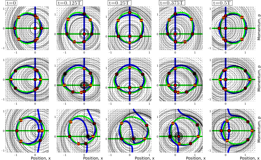
Figure 7: Wigner current patterns $\bm{J}$ (5) for the superposition state $\Psi_{0,1}(t;\frac{\pi}{3})$ for times $t/T^{\mathcal{A}}_{0,1}=0$, $1/8$, $1/4$, $3/8$, $1/2$. The same symbols as in fig. 5 are used (dashed black lines show zeros of $W^{\odot}$). The potentials are (see Table 1) Eckart potential, with $\alpha_{4}^{\cal E}=0.042$ ($D=4$) (top row), Rosen-Morse potential, with $\alpha_{4}^{\cal R}=-0.042$ ($D=4$, $N=8$), and Morse potential, with $\alpha_{3}^{\cal M}=-0.088$ ($D=16$, $N=32$). Note that the Morse potential is odd, i.e. it is hard on the left ($x<0$) and soft on the right side ($x>0$); accordingly, the current patterns on the left resemble those of the Eckart potential depicted (top row) and those on the right resemble those for the Rosen-Morse potential (middle row).

Figure 8: Demonstration of conservation of current winding number for fixed time $t=T/8$ parameterized using a varying weighting angle $\theta$ of superposition state $\Psi_{0,1}(x,\frac{T}{8};\theta)$ (dashed black lines show zeros of $W^{\odot}$). We observe movements of stagnation points leading to their merger and splitting. The top row refers to the hard Eckart and bottom row to the soft Rosen-Morse potential with identical parameters as in fig. 7. Note the non-Liouvillian nature of the current Kakofengitis et al. (2017) featuring regions of pronounced expansion and compression.

VI.2 The Ferris Wheel Effect – alignment with $x$- and $p$-axes

According to the discussion in Section V.2, four diagonal stagnation points form per zero-circle of every eigenstate. If we ‘perturb’ an eigenstate by, say, mixing in a little bit of groundstate ($\Psi_{m,0}(\theta)$ of Eq. (1) with $\theta\ll 1$), the zero-circle gets displaced from the origin [see Eq. (10)]. Yet, for small values of $\theta$ the four diagonal stagnation points remain pinned to the zero-circle while it rotates around the origin as time progresses. They do this such that they maintain their relative orientation with respect to the axes of phase-space, as seen from the zero-circle’s centre. In other words, while they travel through phase-space they behave somewhat like markers on a Ferris wheel cabin, where the zero-line, $J_{x}=0$, depicts the cabin’s outline, see fig. 7.

VI.3 Rabi scenario: modified two-state dynamics

To investigate a simple system in which the weighting angle $\theta$ of the superposition state (1) changes considerably while the dynamics progresses, we study a resonantly driven Rabi system. Its solution for a superposition of ground and first excited state is

$$\Psi^{R}_{0,1}(x,t;\theta(t))=\Psi_{0,1}(x,t;\frac{\Omega_{R}}{2}t+\frac{\pi}{2})\;,$$ (17)

where $\Omega_{R}$ is the Rabi frequency Walls and Milburn (1994) and the rotating wave approximation has been used. In accord with this approximation we assume that the perturbation is so small that we can neglect the time-dependence of the Hamiltonian when determining the fieldlines of $\bm{J}$.

The Rabi state (17) displays Wigner current patterns associated with the system’s (fast) intrinsic dynamics while (slowly) shifting the weighting of the superposition state: for the ratio of these two system frequencies we choose $\frac{\Omega_{R}}{\Omega^{\odot}}=\frac{1}{8}$ in fig. 9.

To monitor the effects of the slow shift of $\theta$ by itself we keep time fixed and change $\theta$ ‘by hand’. The topological nature of the stagnation points conserves the current winding number in this case as well, see fig. 8.

For the full time-dependence we choose $\frac{\Omega_{R}}{\Omega^{\odot}}=\frac{1}{8}$ in fig. 9. It shows plots with zero-circles (10) tied to a spiral centred on $t=0$ (since $\Psi^{R}_{0,1}(t=0)=\psi_{1}$) which expands outward as more of the groundstate gets mixed in with increasing values of $|t|$. We notice that the Ferris wheel-effect tends to keep the orientation of the stagnation points on the zero circle aligned with $x$- and $p$-axes. With our choice of $\frac{\Omega_{R}}{\Omega^{\odot}}=\frac{1}{8}$, around $|t|=2T$ the mixing angle is roughly $|\theta|=\frac{\pi}{4}$. At this stage the zero-circle gets displaced by its radius and stagnation points on the circle interact with those on $x$- and $p$-axes, see fig. 9, displaying repulsion, attraction, coalescence and splitting of stagnation points– all constrained by conservation of topological charge.

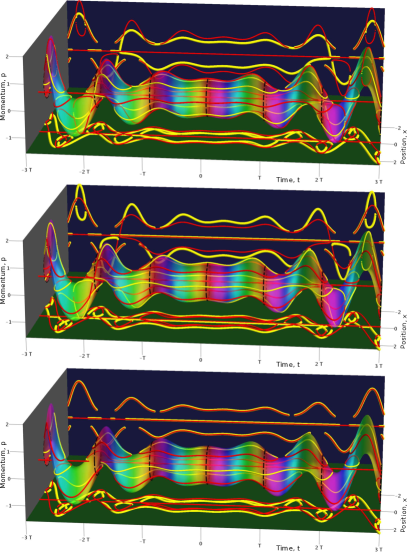
Figure 9: Rabi scenario for state (17) with frequency ratio $\Omega_{R}/\Omega^{\odot}=1/8$. The panels feature, from top to bottom, a soft, hard and odd potential, Table 1, with respective anharmonicity values, $\alpha_{4}^{\cal E}=0.002$, $\alpha_{4}^{\cal R}=-0.002$ and $\alpha_{3}^{\cal M}=-0.004$. At time $t=0$ the system is in the first excited state; at other times the zero-circle’s center (10) is displaced from the origin such that, over time, it sweeps out a helix with varying width. This is displayed as a helical tube whose rainbow coloring depicts the flow of time. Every full period ($T^{\odot}=1$) is denoted by a dashed black zero-circle. Stagnation points are depicted by red lines when carrying charge $\omega=+1$ and yellow if $\omega=-1$, compare fig. 1. The stagnation point positions are additionally projected along the $x$-axis onto the blue wall in the back and along the $p$-axis downward onto the green floor. Winding number conservation implies that positively and negatively charged stagnation points originate and annihilate together, this is seen as red and yellow lines forming loops which are reminiscent of the formation of the torus reported in fig. 4 of reference Steuernagel et al. (2013). As mentioned in fig. 5 above, the bottom panel, for the odd Morse potential, inherits features of Rosen-Morse and Eckart potentials.

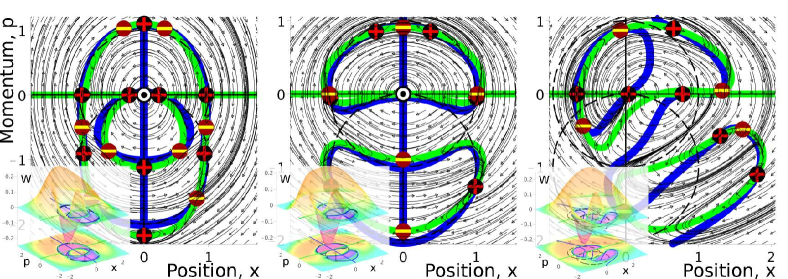
Figure 10: Wigner current pattern for state $\Psi_{1,2}\left(x,\frac{3T}{4};\frac{\pi}{4}\right)$ for, from left to right, Eckart, Rosen-Morse and Morse potentials, Table 1, with respective anharmonicity values $\alpha_{4}^{\cal E}=0.042$ ($D=4$), $\alpha_{4}^{\cal R}=0.033$ ($D=5$, $N=10$), and $\alpha_{3}^{\cal M}=0.125$ ($D=8$, $N=16$). The same symbols as in fig. 5 are used (dashed black lines show zeros of $W^{\odot}$). Zeros of the Wigner distribution (thick green lines) intersect with zeros of the momentum component of Wigner current (thick blue line) yielding fairly intricate arrangements of stagnation points of Wigner current. Similarly to Figs. 5 and 9, the Morse potential’s case inherits features of a stiff potential for $x<0$ and of a soft potential for $x>0$.

VI.4 Other Superpositions

Other superposition states, such as $\Psi_{1,2}$, can show symmetric flower petal arrangements, see insets in fig. 10, which have recently been observed experimentally Hofheinz et al. (2009). fig. 10 shows how the three different types of weakly-anharmonic potentials give rise to current patterns which generalise our previous discussions in Sections V.2 and VI.2.

VII Motivation and conclusion

Our investigations of Wigner current $\bm{J}$ and its fieldlines shows that they give us insights into quantum phase-space dynamics:

$\bm{J}$-fieldlines provide visualisation at-a-glance, in this sense, their collection across phase-space are quantum analogs of classical phase-space trajectories.

$\bm{J}$ and collections of its fieldlines reveal subtle patterns in phase-space dynamics, such as contracting and expanding regions of phase-space, current stagnation points, loops, separatrices and saddles; similar to classical phase portraits Cvitanović et al. (2012); Nolte (2010).

In contrast to classical phase space current, $\bm{J}$ is non-Liouvillian Kakofengitis et al. (2017), compare e.g. fig. 8.

$\bm{J}$ can be characterised by its stagnation points’ distribution and Poincaré-Hopf-indices.

$\bm{J}$-fieldlines follow neither energy-contours nor Wigner distribution-contours Oliva et al. .

They allow us to check concepts such as Wigner ‘trajectories’ and dismiss such concepts Oliva et al. ; Kakofengitis et al. (2017).

Phase-space quantum mechanics is useful for approximate numerical modelling of quantum dynamics using semi-classical approximations, particularly in theoretical quantum chemistry, for a good and brief recent overview see Koda (2015) and references therein.

Wigner current and its fieldlines allow us to benchmark approximate propagation schemes Donoso and Martens (2001); Donoso et al. (2003); Cabrera et al. (2015) against the full theory.

We expect that investigations of Wigner current will lead to new insights into the nature of chaotic systems Berry (1987) and quantum-classical correspondences Jaffé et al. (1985).

We have shown that in the case of vanishing Planck constant $\hbar$ or vanishing anharmonicity, $\bm{J}$ does not pointwise converge to classical dynamics, see Section V.1.

We expect Wigner current $\bm{J}$ and collections of its fieldlines to become a widely used tool for the study of quantum dynamics – similar to classical phase portraits.

References

- Berry (1978) M. V. Berry, in Am. Inst. Phys. Conf. Ser., Vol. 46 (1978) pp. 16–120.
- Cvitanović et al. (2012) P. Cvitanović, R. Artuso, R. Mainieri, G. Tanner, and G. Vattay, Chaos: Classical and Quantum (ChaosBook.org, Niels Bohr Institute, Copenhagen, 2012).
- (3) M. Oliva, D. Kakofengitis, and O. Steuernagel, 1611.03303 .
- Wigner (1932) E. Wigner, Phys. Rev. 40, 749 (1932).
- Zachos (2002) C. Zachos, Int. J. Mod. Phys. A 17, 297 (2002), arXiv:hep-th/0110114 .
- Hirshfeld and Henselder (2002) A. C. Hirshfeld and P. Henselder, Am. J. Phys. 70, 537 (2002), arXiv:quant-ph/0208163 .
- Hancock et al. (2004) J. Hancock, M. A. Walton, and B. Wynder, Eur. J. Phys. 25, 525 (2004), arXiv:physics/0405029 .
- Rasinariu (2013) C. Rasinariu, Fortsch. Phys. 61, 4 (2013), arXiv:1204.6495 .
- Zachos et al. (2005) C. K. Zachos, D. B. Fairlie, and T. L. Curtright, World Scientific 34 (2005), 10.1142/5287.
- Hillery et al. (1984) M. Hillery, R. F. O’Connell, M. O. Scully, and E. P. Wigner, Phys. Rep. 106, 121 (1984).
- Case (2008) W. B. Case, Am. J. Phys. 76, 937 (2008).
- Kakofengitis et al. (2017) D. Kakofengitis, M. Oliva, and O. Steuernagel, Phys. Rev. A 95, 022127 (2017), 1611.06891 .
- Groenewold (1946) H. J. Groenewold, Physica 12, 405 (1946).
- Moyal (1949) J. E. Moyal, Proc. Camb. Phil. Soc. 45, 99 (1949).
- Dennis et al. (2009) M. R. Dennis, K. O’Holleran, and M. J. Padgett, in ”Progress in Optics”, Vol. 53, edited by E. Wolf (Elsevier, 2009) pp. 293 – 363.
- Royer (1992) A. Royer, Found. Phys. 22, 727 (1992).
- Ballentine et al. (1994) L. E. Ballentine, Y. Yang, and J. P. Zibin, Phys. Rev. A 50, 2854 (1994).
- Zurek (2001) W. H. Zurek, Nature 412, 712 (2001), arXiv:quant-ph/0201118 .
- Steuernagel et al. (2013) O. Steuernagel, D. Kakofengitis, and G. Ritter, Phys. Rev. Lett. 110, 030401 (2013), 1208.2970 .
- Donoso and Martens (2001) A. Donoso and C. C. Martens, Phys. Rev. Lett. 87, 223202 (2001).
- Schleich (2001) W. P. Schleich, Quantum Optics in Phase Space (Wiley-VCH, New York, 2001).
- (22) H. Bauke and N. R. Itzhak, 1101.2683 .
- Berry (2000) M. V. Berry, Nature 403, 21 (2000).
- Peder Dahl and Springborg (1988) J. Peder Dahl and M. Springborg, J. Chem. Phys. 88, 4535 (1988).
- Takabayasi (1954) T. Takabayasi, Prog. Theo. Phys. 11, 341 (1954).
- Dutt et al. (1988) R. Dutt, A. Khare, and U. P. Sukhatme, Am. J. Phys. 56, 163 (1988).
- Daligault (2003) J. Daligault, Phys. Rev. A 68, 010501 (2003).
- Lee and Scully (1982) H. Lee and M. O. Scully, J. Chem. Phys. 77, 4604 (1982).
- Walls and Milburn (1994) D. F. Walls and G. J. Milburn, Quantum Optics (Springer, 1994).
- Hofheinz et al. (2009) M. Hofheinz, H. Wang, M. Ansmann, R. C. Bialczak, E. Lucero, M. Neeley, A. D. O’Connell, D. Sank, J. Wenner, J. M. Martinis, and A. N. Cleland, Nature 459, 546 (2009).
- Nolte (2010) D. D. Nolte, Phys. Today 63, 33 (2010).
- Koda (2015) S.-I. Koda, J. Chem. Phys. 143, 244110 (2015).
- Donoso et al. (2003) A. Donoso, Y. Zheng, and C. C. Martens, J. Chem. Phys. 119, 5010 (2003).
- Cabrera et al. (2015) R. Cabrera, D. I. Bondar, K. Jacobs, and H. A. Rabitz, Phys. Rev. A 92, 042122 (2015), 1212.3406 .
- Berry (1987) M. V. Berry, Royal Soc. London Proc. Series A 413, 183 (1987).
- Jaffé et al. (1985) C. Jaffé, S. Kanfer, and P. Brumer, Phys. Rev. Lett. 54, 8 (1985).