Probing of quantum turbulence with radiating vortex loops

Abstract

The statistics of vortex loops emitted from the domain with quantum turbulence is studied. The investigation is performed on the supposition that the vortex loops have the Brownian or random walking structure with the generalized Wiener distribution. The main goal is to relate the properties of the emitted vortex loops with the parameters of quantum turbulence. The motivation of this work connected with recent studies, both numerical and experimental, on study of emitted vortex loops. This technique opens up new opportunities to probe superfluid turbulence. We demonstrated how the statistics of emitted loops is expressed in terms of the vortex tangle parameters and performed the comparison with numerical simulations.
PACS number(s): 67.25.dk, 47.37.+q

Scientific Background and motivations. Quantum turbulence (QT) in superfluids is one of the most fascinating phenomena in the theory of quantum fluids Nemirovskii (2013). In general, the vortex tangle composing QT, consists of a set of vortex loops of different lengths and having a random structure. Question of an arrangement of the vortex tangle is a key problem of the theory of QT. Recently, a number of works devoted to the study of the vortex tangle structure with the use of emitted from the turbulent domain have been performed Nakatsuji et al. (2014),Nago et al. (2013),Kondaurova and Nemirovskii (2012),Walmsley et al. (2013). This technique opens up new opportunities for research QT.

One of the main problem in this activity is to relate the properties of the emitted vortex loops with the parameters of quantum turbulence. In the present work we propose an analytical approach that allows to relate the statistics of vortex loops with the parameters of the real vortex tangle This approach is based on the Gaussian model of the vortex tangle, which describes the latter as a set of vortex loops having a random walking structure with the generalized Wiener distribution,Nemirovskii (2008). Then we apply our results for data processing of numerical work Nakatsuji et al. (2014) who studied quantum turbulence driven by an oscillating sphere. Generation of quantum turbulence by oscillating objects is very important topic in this field (see, e.g. Chagovets et al. (2009),Sheshin et al. (2008),Gritsenko and Sheshin (2014))

Flux of vortex loops emitted from quantum turbulence. In this paragraph we very briefly describe main ideas leading to the theory of emission of vortex loops, details can be found in paper by the author Nemirovskii (2010). Vortex loops composing the vortex tangle can move as a whole with a drift velocity $V_{l}$ depending on their structure and their length $l$. The flux of the line length, energy, momentum etc., executed by the moving vortex loops takes place. In the case of inhomogeneous vortex tangle the net flux $\mathbf{J}$ of the vortex length due to the gradient of concentration of the vortex line density $\mathcal{L}(x,t)$ appears. The situation here is exactly the same as in classical kinetic theory with the difference being that the ”carriers” are not the point particles but the extended objects (vortex loops), which possess an infinite number of degrees of freedom with very involved dynamics.

To develop the theory of the transport processes fulfilled by vortex loops (in spirit of classical kinetic theory) we need to know the drift velocity $V_{l}$ and the free path $\lambda(l)$ for the loop of size $l$. Referring to the paper Nemirovskii (2010) we write down here the following result. The drift velocity $V_{l}$  and the free path $\lambda(l)$ for the loop of size $l$ are

$$V_{l}=C_{v}\beta/\sqrt{l\xi_{0}},\ \ \ \lambda(l)=1/2lb_{m}\mathcal{L}.$$ (1)

Quantity $\beta$ is $(\kappa/4\pi)\ln(\mathcal{L}^{-1/2}/a_{0})$, where $\kappa$ is the quantum of circulation and $a_{0}$ is the core radius, $C_{v}$ is numerical factor of the order of unity, $b_{m}$ is the numerical factor , approximately equal to $\ b_{m}\approx 0.2$ . The $\xi_{0}$ is the parameter of the generalized Wiener distribution, it is of order of the interline space $\mathcal{L}^{-1/2}.$ The probability $P(x)$ for the loop of length $l$ to fly the distance $x$ without collision is $P(x)=(1/\lambda(l))\exp(-x/\lambda(l))$. Knowing the averaged velocity $V_{l}$ of loops, and the probability $P(x)$ (both quantities are $l$ -dependent), we can evaluate the spatial flux $\mathbf{J}$ of the vortex loops.

Let us consider the small area element placed at some point of the boundary of domain containing QT and oriented perpendicularly to axis $x$ (See for details Fig.2 of paper Nemirovskii (2010)). The $x$ component of flux $\mathbf{J}$ of the number of loops executed by loops of sizes $l,$ placed in $\theta,\varphi$ direction, and remote from the area element at distance $R,$ can be written as:

$$J_{x}(l)=\frac{1}{4\pi}\int n(l,R,\theta,\varphi)(V_{l}\cos\theta)P(R)\sin\theta d\theta d\varphi dR.$$ (2)

Here the quantity $(V_{l}\cos\theta)$ is just the $x$ component of the drift velocity, the factor $P(R)dR$ is introduced to control an attenuation of flux, due to collisions. In the spirit of classical kinetic theory, we assume the local equilibrium is established.

In paper Nemirovskii (2010)  Eq. ( 2) was the starting point to develop the theory of diffusion of vortex loops in quantum turbulence, therefore the density of loops $n(l)$ was supposed to depend on spacial position, in spherical coordinates $n=n(l,R,\theta,\varphi)$). Here we put another goal to study radiation of loops from the domain with uniform vortex tangle. Supposing that inside domain the density of loops does not depend on spatial coordinates ($n(l,R,\theta,\varphi)=n(l))$, and integrating out over solid angle $d\theta d\varphi$ and over position of loops $dR$ we obtain the $x$-component of the loop flux through the domain boundary

$$J_{x}=\frac{1}{4}\int n(l)(\frac{\beta}{\sqrt{l\xi_{0}}})dl.$$ (3)

The flux $J_{x}$, described by formula 3 carries the loops of different sizes in the normal to boundary direction and provides information on the distribution of loops inside of the turbulent domain. However, since the speed of loops depends on their sizes the initial distribution changes as the vortex ”cloud” propagates. For instance, in some time the small vortex loops (practically rings) get ahead, and the measurements in a short time will detect only small loops. That means that the experimental data essentially depends on the position of detector and time time of registration. In a stationary situation when the turbulence is maintained by some means (counterflow or oscillating structures), the intensity of detected loops should be steady in time.

Processing of experimental and numerical works. As an illustration let’s treat the numerical work Nakatsuji et al. (2014) on the statistics of emitted loops. Unfortunately, the pure experimental works are not too reliable for a proper quantitative treatment. In work Nakatsuji et al. (2014) the authors have studied the statistics of vortex loops emitted from quantum turbulence driven by an oscillating sphere of radius $1\mu m$ with the frequency $3$ kHz, and the amplitude $5.31$ $\mu m$,. Counting of loops was made on the spherical boundary of radius 30 $\mu m$ (centered at the center of the oscillating sphere). The result of this counting is illustrated in the left graph in Fig.1 ,where the a probability density function (PDF) $\Pr_{num}(l)$ of the length of the emitted vortex loops is presented.

Let us try to consider this result from the position of the theory stated above. Formula 3 describes the flux of loops per unit area. The integrand in 3 is distribution of loops over their lengths in the propagating loop ”jet”. The total number of emitted loops (per unit time) is $N(l)=\int\mathbf{J}d\mathbf{S}$. The Gaussian model, used in our consideration predicts that the density of loops $n(l)$ inside the domain with vortex tangle is the power-like function $n(l)=Al^{-5/2}$. This behaviour, however, has a low cutoff near the length $l\thicksim\xi_{0}$. Below the cutoff there are a few loops of smaller sizes which do not essentially affect the whole theory. From the graph for PDF $\Pr_{num}(l)$ in Fig. 1 it is seen that the cutoff is $l\approx 5\ \mu m$. The size $l\approx 5\ \mu m$ is the point of the maximum of the PDF $\Pr_{num}(l)$, where the power-like behaviour ceases. Using 3 we get that the analytical PDF is $\Pr_{an}(l)=N(l)/\int N(l)dl\varpropto l^{-3}$. Furthermore, taking into account that in the normalization factor $\int N(l)dl$, the value of integral is accumulated near the lower limit $l\thicksim 5\ \mu m$, we get that the analytical PDF approximatel is $\Pr_{an}(l)\approx 50l^{-3}$.

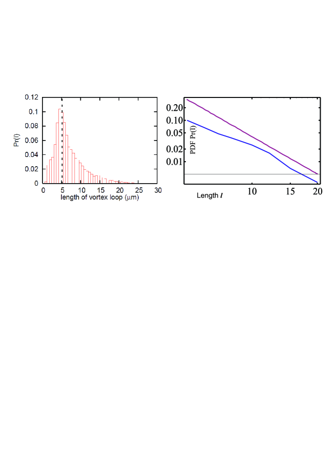
Figure 1: (Color online) Left. The PDF of the length of emitted vortex loops obtained in Nakatsuji et al. (2014). Right. Lower line is the PDF from the left picture depicted in logarithmic coordinates. The upper curve is the analytical PDF $\Pr_{an}(l)\approx 50l^{-3}$, obtained in this work.

In the right picture of Fig 1 we depicted PDF $\Pr_{num}(l)$ obtained in work Nakatsuji et al. (2014) and our $\Pr_{an}(l)\approx 50l^{-3}$ in the logarithmic coordinates. It can be seen that the power $-3$ is indeed close to the numerical data, deviations appear near the low cutoff where the Gaussian model does not work properly. As for absolute values of the PDFs (numerical and analytical) they differ by a factor about $2\div 3$ (for large loops). This can be explained by the fact that the vortex turbulence, produced in numerical simulation is not the dense and uniform structure, which was required in the analytical consideration. In fact, the interline space obained from the data on total length (see Fig. 2 of paper Nakatsuji et al. (2014)) is about $20\mu m$ which is comparable with size of largest loops. This implies that the VT is rather dilute.

Conclusion. Summarizing we can conclude that the ”clouds” of vortex loops emitted from the turbulent superfluid helium provides an important information on the structure of QT. However, due to very complicated dynamics of the network of vortex loops, this information is hidden and should be extracted with the use of appropriate formalism. It should be understood that the described above procedure is greatly simplified, many real features such as a possible anisotropy, the mutual friction, the specific conditions of the turbulence generation have not been considered. This is supposed to be performed in future.

The study was performed by grant from the Russian Science Foundation (project N 14-29-00093) and by grant 13-08-00673 from RFBR (Russian Foundation of Fundamental Research).

References

- (1)
- (2)
- (3)
- (4)
- Nemirovskii (2013) S. K. Nemirovskii, Physics Reports 524, 85 (2013).
- Nakatsuji et al. (2014) A. Nakatsuji, M. Tsubota, and H. Yano, Phys. Rev. B 89, 174520 (2014).
- Nago et al. (2013) Y. Nago, A. Nishijima, H. Kubo, T. Ogawa, K. Obara, H. Yano, O. Ishikawa, and T. Hata, Phys. Rev. B 87, 024511 (2013).
- Kondaurova and Nemirovskii (2012) L. Kondaurova and S. K. Nemirovskii, Phys. Rev. B 86, 134506 (2012).
- Walmsley et al. (2013) P. M. Walmsley, P. A. Tompsett, D. E. Zmeev, and A. I. Golov, ArXiv e-prints (2013), eprint 1308.6171.
- Nemirovskii (2008) S. K. Nemirovskii, Phys. Rev. B 77, 214509 (2008).
- Chagovets et al. (2009) V. Chagovets, I. Gritsenko, E. Rudavskii, G. Sheshin, A. Zadorozhko, and B. Verkin, Journal of Physics: Conference Series 150, 032014 (2009).
- Sheshin et al. (2008) G. A. Sheshin, A. A. Zadorozhko, . Y. Rudavskii, V. K. Chagovets, L. Skrbek, and M. Blazhkova, Low Temperature Physics 34, 875 (2008).
- Gritsenko and Sheshin (2014) I. Gritsenko and G. Sheshin, Journal of Low Temperature Physics 175, 91 (2014).
- Nemirovskii (2010) S. K. Nemirovskii, Phys. Rev. B 81, 064512 (2010).