Minimal discs in hyperbolic space bounded by a quasicircle at infinity

Abstract.

We prove that the supremum of principal curvatures of a minimal embedded disc in hyperbolic three-space spanning a quasicircle in the boundary at infinity is estimated in a sublinear way by the norm of the quasicircle in the sense of universal Teichmüller space, if the quasicircle is sufficiently close to being the boundary of a totally geodesic plane. As a by-product we prove that there is a universal constant C independent of the genus such that if the Teichmüller distance between the ends of a quasi-Fuchsian manifold $M$ is at most C, then $M$ is almost-Fuchsian. The main ingredients of the proofs are estimates on the convex hull of a minimal surface and Schauder-type estimates to control principal curvatures.

1. Introduction

Let $\mathbb{H}^{3}$ be hyperbolic three-space and $\partial_{\infty}\mathbb{H}^{3}$ be its boundary at infinity. A surface $S$ in hyperbolic space is minimal if its principal curvatures at every point $x$ have opposite values. We will denote the principal curvatures by $\lambda$ and $-\lambda$, where $\lambda=\lambda(x)$ is a nonnegative function on $S$. It was proved by Anderson ([And83, Theorem 4.1]) that for every Jordan curve $\Gamma$ in $\partial_{\infty}\mathbb{H}^{3}$ there exists a minimal embedded disc $S$ whose boundary at infinity coincides with $\Gamma$. It can be proved that if the supremum $||\lambda||_{\infty}$ of the principal curvatures of $S$ is in $(-1,1)$, then $\Gamma=\partial_{\infty}S$ is a quasicircle, namely $\Gamma$ is the image of a round circle under a quasiconformal map of the sphere at infinity.

However, uniqueness does not hold in general. Anderson proved the existence of a Jordan curve $\Gamma\subset\partial_{\infty}\mathbb{H}^{3}$ invariant under the action of a quasi-Fuchsian group $G$ spanning several distinct minimal embedded discs, see [And83, Theorem 5.3]. In this case, $\Gamma$ is a quasicircle and coincides with the limit set of $G$. More recently in [HW13a] invariant curves spanning an arbitrarily large number of minimal discs were constructed. On the other hand, if the supremum of the principal curvatures of a minimal embedded disc $S$ satisfies $||\lambda||_{\infty}\in(-1,1)$ then, by an application of the maximum principle, $S$ is the unique minimal disc asymptotic to the quasicircle $\Gamma=\partial_{\infty}S$.

The aim of this paper is to study the supremum $||\lambda||_{\infty}$ of the principal curvatures of a minimal embedded disc, in relation with the norm of the quasicircle at infinity, in the sense of universal Teichmüller space. The relations we obtain are interesting for “small” quasicircles, that are close in universal Teichmüller space to a round circle. The main result of this paper is the following:

Theorem A.

There exist universal constants $K_{0}>1$ and $C>0$ such that every minimal embedded disc in $\mathbb{H}^{3}$ with boundary at infinity a $K$-quasicircle $\Gamma\subset\partial_{\infty}\mathbb{H}^{3}$, with $1\leq K\leq K_{0}$, has principal curvatures bounded by

$$||\lambda||_{\infty}\leq C\log K\,.$$

Recall that the minimal disc with prescribed quasicircle at infinity is unique if $||\lambda||_{\infty}<1$. Hence we can draw the following consequence, by choosing $K_{0}^{\prime}<\min\{K_{0},e^{1/C}\}$:

Theorem B.

There exists a universal constant $K^{\prime}_{0}$ such that every $K$-quasicircle $\Gamma\subset\partial_{\infty}\mathbb{H}^{3}$ with $K\leq K^{\prime}_{0}$ is the boundary at infinity of a unique minimal embedded disc.

Applications to quasi-Fuchsian manifolds

Theorem A has a direct application to quasi-Fuchsian manifolds. Recall that a quasi-Fuchsian manifold $M$ is isometric to the quotient of $\mathbb{H}^{3}$ by a quasi-Fuchsian group $G$, isomorphic to the fundamental group of a closed surface $\Sigma$, whose limit set is a Jordan curve $\Gamma$ in $\partial_{\infty}\mathbb{H}^{3}$. The topology of $M$ is $\Sigma\times{\mathbb{R}}$. We denote by $\Omega_{+}$ and $\Omega_{-}$ the two connected components of $\partial_{\infty}\mathbb{H}^{3}\setminus\Gamma$. Then $\Omega_{+}/G$ and $\Omega_{-}/G$ inherit natural structures of Riemann surfaces on $\Sigma$ and therefore determine two points of $\mathcal{T}(\Sigma)$, the Teichmüller space of $\Sigma$. Let $d_{\mathcal{T}(\Sigma)}$ denote the Teichmüller distance on $\mathcal{T}(\Sigma)$.

Corollary A.

There exist universal constants $C>0$ and $d_{0}>0$ such that, for every quasi-Fuchsian manifold $M=\mathbb{H}^{3}/G$ with $d_{\mathcal{T}(\Sigma)}(\Omega_{+}/G,\Omega_{-}/G)<d_{0}$ and every minimal surface $S$ in $M$ homotopic to $\Sigma\times\{0\}$, the supremum of the principal curvatures of $S$ satisfies:

$$||\lambda||_{\infty}\leq Cd_{\mathcal{T}(\Sigma)}(\Omega_{+}/G,\Omega_{-}/G)\,.$$

Indeed, under the hypothesis of Corollary A, the Teichmüller map from one hyperbolic end of $M$ to the other is $K$-quasiconformal for $K\leq e^{2d_{0}}$. Hence the lift to the universal cover $\mathbb{H}^{3}$ of any closed minimal surface in $M$ is a minimal embedded disc with boundary at infinity a $K$-quasicircle, namely the limit set of the corresponding quasi-Fuchsian group. Choosing $d_{0}=(1/2)\log K_{0}$, where $K_{0}$ is the constant of Theorem A, and choosing $C$ as in Theorem A (up to a factor $2$ which arises from the definition of Teichmüller distance), the statement of Corollary A follows.

We remark here that the constant $C$ of Corollary A is independent of the genus of $\Sigma$.

A quasi-Fuchsian manifold contaning a closed minimal surface with principal curvatures in $(-1,1)$ is called almost-Fuchsian, according to the definition given in [KS07]. The minimal surface in an almost-Fuchsian manifold is unique, by the above discussion, as first observed by Uhlenbeck ([Uhl83]). Hence, applying Theorem B to the case of quasi-Fuchsian manifolds, the following corollary is proved.

Corollary B.

If the Teichmüller distance between the conformal metrics at infinity of a quasi-Fuchsian manifold $M$ is smaller than a universal constant $d_{0}^{\prime}$, then $M$ is almost-Fuchsian.

Indeed, it suffices as above to pick $d_{0}^{\prime}=(1/2)\log K_{0}^{\prime}$, which is again independent on the genus of $\Sigma$. By Bers’ Simultaneous Uniformization Theorem, the Riemann surfaces $\Omega_{\pm}/G$ determine the manifold $M$. Hence the space $\mathcal{QF}(\Sigma)$ of quasi-Fuchsian manifolds homeomorphic to $\Sigma\times{\mathbb{R}}$, considered up to isometry isotopic to the identity, can be identified to $\mathcal{T}(\Sigma)\times\mathcal{T}(\Sigma)$. Under this identification, the subset of $\mathcal{QF}(\Sigma)$ composed of Fuchsian manifolds, which we denote by $\mathcal{F}(\Sigma)$, coincides with the diagonal in $\mathcal{T}(\Sigma)\times\mathcal{T}(\Sigma)$. Let us denote by $\mathcal{AF}(\Sigma)$ the subset of $\mathcal{QF}(\Sigma)$ composed of almost-Fuchsian manifolds. Corollary B can be restated in the following way:

Corollary C.

There exists a uniform neighborhood $N(\mathcal{F}(\Sigma))$ of the Fuchsian locus $\mathcal{F}(\Sigma)$ in $\mathcal{QF}(\Sigma)\cong\mathcal{T}(\Sigma)\times\mathcal{T}(\Sigma)$ such that $N(\mathcal{F}(\Sigma))\subset\mathcal{AF}(\Sigma)$.

We remark that Corollary A is a partial converse of results presented in [GHW10], giving a bound on the Teichmüller distance between the hyperbolic ends of an almost-Fuchsian manifold in terms of the maximum of the principal curvatures. Another invariant which has been studied in relation with the properties of minimal surfaces in hyperbolic space is the Hausdorff dimension of the limit set. Corollary A and Corollary B can be compared with the following theorem given in [San14]: for every $\epsilon$ and $\epsilon_{0}$ there exists a constant $\delta=\delta(\epsilon,\epsilon_{0})$ such that any stable minimal surface with injectivity radius bounded by $\epsilon_{0}$ in a quasi-Fuchsian manifold $M$ are in $(-\epsilon,\epsilon)$ provided the Hausdorff dimension of the limit set of $M$ is at most $1+\delta$. In particular, $M$ is almost Fuchsian if one chooses $\epsilon<1$. Conversely, in [HW13b] the authors give an estimate of the Hausdorff dimension of the limit set in an almost-Fuchsian manifold $M$ in terms of the maximum of the principal curvatures of the (unique) minimal surface. The degeneration of almost-Fuchsian manifolds is also studied in [San13].

The main steps of the proof

The proof of Theorem A is composed of several steps.

By using the technique of “description from infinity” (see [Eps84] and [KS08]), we construct a foliation $\mathcal{F}$ of $\mathbb{H}^{3}$ by equidistant surfaces, such that all the leaves of the foliation have the same boundary at infinity, a quasicircle $\Gamma$. By using a theorem proved in [ZT87] and [KS08, Appendix], which relates the curvatures of the leaves of the foliation with the Schwarzian derivative of the map which uniformizes the conformal structure of one component of $\partial_{\infty}\mathbb{H}^{3}\setminus\Gamma$, we obtain an explicit bound for the distance between two surfaces $F_{+}$ and $F_{-}$ of $\mathcal{F}$, where $F_{+}$ is concave and $F_{-}$ is convex, in terms of the Bers norm of $\Gamma$. The distance $d_{\mathbb{H}^{3}}(F_{-},F_{+})$ goes to $0$ when $\Gamma$ approaches a circle in $\partial_{\infty}\mathbb{H}^{3}$.

A fundamental property of a minimal surface $S$ with boundary at infinity a curve $\Gamma$ is that $S$ is contained in the convex hull of $\Gamma$. The surfaces $F_{-}$ and $F_{+}$ of the previous step lie outside the convex hull of $\Gamma$, on the two different sides. Hence every point $x$ of $S$ lies on a geodesic segment orthogonal to two planes $P_{-}$ and $P_{+}$ (tangent to $F_{-}$ and $F_{+}$ respectively) such that $S$ is contained in the region bounded by $P_{-}$ and $P_{+}$. The length of such geodesic segment is bounded by the Bers norm of the quasicircle at infinity, in a way which does not depend on the chosen point $x\in S$.

The next step in the proof is then a Schauder-type estimate. Considering the function $u$, defined on $S$, which is the hyperbolic sine of the distance from the plane $P_{-}$, it turns out that $u$ solves the equation

($$\star \Delta_{S}u-2u=0\,,$$ ‣ 2.4)

where $\Delta_{S}$ is the Laplace-Beltrami operator of $S$. We then apply classical theory of linear PDEs, in particular Schauder estimates, to the equation $\eqref{lap 2u hyp}$ in order to prove that

$$||u||_{C^{2}(\Omega^{\prime})}\leq C||u||_{C^{0}(\Omega)}\,,$$

where $\Omega^{\prime}\subset\!\subset\Omega$ and $u$ is expressed in normal coordinates centered at $x$. Recall that $\Delta_{S}$ is the Laplace-Beltrami operator, which depends on the surface $S$. In order to have this kind of inequality, it is then necessary to control the coefficients of $\Delta_{S}$. This is obtained by a compactness argument for conformal harmonic mappings, adapted from [Cus09], recalling that minimal discs in $\mathbb{H}^{3}$ are precisely the image of conformal harmonic mapping from the disc to $\mathbb{H}^{3}$. However, to ensure that compact sets in the conformal parametrization are comparable to compact sets in normal coordinates, we will first need to prove a uniform bound of the curvature. For this reason we will assume (as in the statement of Theorem A) that the minimal discs we consider have boundary at infinity a $K$-quasicircle, with $K\leq K_{0}$.

The final step is then an explicit estimate of the principal curvatures at $x\in S$, by observing that the shape operator can be expressed in terms of $u$ and the first and second derivatives of $u$. The Schauder estimate above then gives a bound on the principal curvatures just in terms of the supremum of $u$ in a geodesic ball of fixed radius centered at $x$. By using the first step, since $S$ is contained between $P_{-}$ and the nearby plane $P_{+}$, we finally get an estimate of the principal curvatures of a minimal embedded disc only in terms of the Bers norm of the quasicircle at infinity.

All the previous estimates do not depend on the choice of $x\in S$. Hence the following theorem is actually proved.

Theorem C.

There exist constants $K_{0}>1$ and $C>4$ such that the principal curvatures $\pm\lambda$ of every minimal surface $S$ in $\mathbb{H}^{3}$ with $\partial_{\infty}S=\Gamma$ a $K$-quasicircle, with $K\leq K_{0}$, are bounded by:

(1) $$||\lambda||_{\infty}\leq\frac{C||\Psi||_{\mathcal{B}}}{\sqrt{1-C||\Psi||_{\mathcal{B}}^{2}}}\,,$$

where $\Gamma=\Psi(S^{1})$, $\Psi:\widehat{\mathbb{C}}\to\widehat{\mathbb{C}}$ is a quasiconformal map, conformal on $\widehat{\mathbb{C}}\setminus\mathbb{D}$, and $||\Psi||_{\mathcal{B}}$ denotes the Bers norm of $\Psi$.

Observe that the estimate holds in a neighborhood of the identity (which represents circles in $\partial_{\infty}\mathbb{H}^{3}$), in the sense of universal Teichmüller space. Theorem A is then a consequence of Theorem C, using the well-known fact that the Bers embedding is locally bi-Lipschitz.

Organization of the paper

The structure of the paper is as follows. In Section 2, we introduce the necessary notions on hyperbolic space and some properties of minimal surfaces and convex hulls. In Section 3 we introduce the theory of quasiconformal maps and universal Teichmüller space. In Section 4 we prove Theorem A. The Section is split in several subsections, containing the steps of the proof. In Section 5 we discuss how Theorem B, Corollary A, Corollary B and Corollary C follow from Theorem A.

Acknowledgements

I am very grateful to Jean-Marc Schlenker for his guidance and patience. Most of this work was done during my (very pleasent) stay at University of Luxembourg; I would like to thank the Institution for the hospitality. I am very thankful to my advisor Francesco Bonsante and to Zeno Huang for many interesting discussions and suggestions. I would like to thank an anonymous referee for many observations and advices which highly improved the presentation of the paper.

2. Minimal surfaces in hyperbolic space

We consider (3+1)-dimensional Minkowski space ${\mathbb{R}}^{3,1}$ as ${\mathbb{R}}^{4}$ endowed with the bilinear form

(2) $$\langle x,y\rangle=x^{1}y^{1}+x^{2}y^{2}+x^{3}y^{3}-x^{4}y^{4}\,.$$

The hyperboloid model of hyperbolic 3-space is

$$\mathbb{H}^{3}=\left\{x\in{\mathbb{R}}^{3,1}:\langle x,x\rangle=-1,x^{4}>0\right\}.$$

The induced metric from ${\mathbb{R}}^{3,1}$ gives $\mathbb{H}^{3}$ a Riemannian metric of constant curvature -1. The group of orientation-preserving isometries of $\mathbb{H}^{3}$ is $\mathrm{Isom}(\mathbb{H}^{3})\cong\mathrm{SO}_{+}(3,1)$, namely the group of linear isometries of ${\mathbb{R}}^{3,1}$ which preserve orientation and do not switch the two connected components of the quadric $\left\{\langle x,x\rangle=-1\right\}$. Geodesics in hyperbolic space are the intersection of $\mathbb{H}^{3}$ with linear planes $X$ of ${\mathbb{R}}^{3,1}$ (when nonempty); totally geodesic planes are the intersections with linear hyperplanes and are isometric copies of hyperbolic plane $\mathbb{H}^{2}$.

We denote by $d_{\mathbb{H}^{3}}(\cdot,\cdot)$ the metric on $\mathbb{H}^{3}$ induced by the Riemannian metric. It is easy to show that

(3) $$\cosh(d_{\mathbb{H}^{3}}(p,q))=|\langle p,q\rangle|$$

and other similar formulae which will be used in the paper.

Note that $\mathbb{H}^{3}$ can also be regarded as the projective domain

$$P(\left\{\langle x,x\rangle<0\right\})\subset{\mathbb{R}}P^{3}.$$

Let us denote by $\widehat{\mathrm{d}\mathbb{S}^{3}}$ the region

$$\widehat{\mathrm{d}\mathbb{S}^{3}}=\left\{x\in{\mathbb{R}}^{3,1}:\langle x,x\rangle=1\right\}$$

and we call de Sitter space the projectivization of $\widehat{\mathrm{d}\mathbb{S}^{3}}$,

$$\mathrm{d}\mathbb{S}^{3}=P(\left\{\langle x,x\rangle>0\right\})\subset{\mathbb{R}}P^{3}.$$

Totally geodesic planes in hyperbolic space, of the form $P=X\cap\mathbb{H}^{3}$, are parametrized by the dual points $X^{\perp}$ in $\mathrm{d}\mathbb{S}^{3}\subset{\mathbb{R}}P^{3}$.

In an affine chart $\left\{x_{4}\neq 0\right\}$ for the projective model of $\mathbb{H}^{3}$, hyperbolic space is represented as the unit ball $\left\{(x,y,z):x^{2}+y^{2}+z^{2}<1\right\}$, using the affine coordinates $(x,y,z)=(x^{1}/x^{4},x^{2}/x^{4},x^{3}/x^{4})$. This is called the Klein model; although in this model the metric of $\mathbb{H}^{3}$ is not conformal to the Euclidean metric of ${\mathbb{R}}^{3}$, the Klein model has the good property that geodesics are straight lines, and totally geodesic planes are intersections of the unit ball with planes of ${\mathbb{R}}^{3}$. It is well-known that $\mathbb{H}^{3}$ has a natural boundary at infinity, $\partial_{\infty}\mathbb{H}^{3}=P(\left\{\langle x,x\rangle=0\right\})$, which is a 2-sphere and is endowed with a natural complex projective structure - and therefore also with a conformal structure.

Given an embedded surface $S$ in $\mathbb{H}^{3}$, we denote by $\partial_{\infty}S$ its asymptotic boundary, namely, the intersection of the topological closure of $S$ with $\partial_{\infty}\mathbb{H}^{3}$.

2.1. Minimal surfaces

This paper is mostly concerned with smoothly embedded surfaces in hyperbolic space. Let $\sigma:S\rightarrow\mathbb{H}^{3}$ be a smooth embedding and let $N$ be a unit normal vector field to the embedded surface $\sigma(S)$. We denote again by $\langle{\cdot},{\cdot}\rangle$ the Riemannian metric of $\mathbb{H}^{3}$, which is the restriction to the hyperboloid of the bilinear form (2) of ${\mathbb{R}}^{3,1}$; $\nabla$ and $\nabla^{S}$ are the ambient connection and the Levi-Civita connection of the surface $S$, respectively. The second fundamental form of $S$ is defined as

$$\nabla_{\tilde{v}}\tilde{w}=\nabla^{S}_{\tilde{v}}\tilde{w}+II(v,w)N$$

if $\tilde{v}$ and $\tilde{w}$ are vector fields extending $v$ and $w$. The shape operator is the $(1,1)$-tensor defined as $B(v)=-\nabla_{v}N$. It satisfies the property

$$II(v,w)=\langle B(v),w\rangle\,.$$

Definition 2.1.

An embedded surface $S$ in $\mathbb{H}^{3}$ is minimal if $\mathrm{tr}(B)=0$.

The shape operator is symmetric with respect to the first fundamental form of the surface $S$; hence the condition of minimality amounts to the fact that the principal curvatures (namely, the eigenvalues of $B$) are opposite at every point.

An embedded disc in $\mathbb{H}^{3}$ is said to be area minimizing if any compact subdisc is locally the smallest area surface among all surfaces with the same boundary. It is well-known that area minimizing surfaces are minimal. The problem of existence for minimal surfaces with prescribed curve at infinity was solved by Anderson; see [And83] for the original source and [Cos13] for a survey on this topic.

Theorem 2.2 ([And83]).

Given a simple closed curve $\Gamma$ in $\partial_{\infty}\mathbb{H}^{3}$, there exists a complete area minimizing embedded disc $S$ with $\partial_{\infty}S=\Gamma$.

A key property used in this paper is that minimal surfaces with boundary at infinity a Jordan curve $\Gamma$ are contained in the convex hull of $\Gamma$. Although this fact is known, we prove it here by applying maximum principle to a simple linear PDE describing minimal surfaces.

Definition 2.3.

Given a curve $\Gamma$ in $\partial_{\infty}\mathbb{H}^{3}$, the convex hull of $\Gamma$, which we denote by $\mathcal{CH}(\Gamma)$, is the intersection of half-spaces bounded by totally geodesic planes $P$ such that $\partial_{\infty}P$ does not intersect $\Gamma$, and the half-space is taken on the side of $P$ containing $\Gamma$.

Hereafter $\mathrm{Hess}\,u$ denotes the Hessian of a smooth function $u$ on the surface $S$, i.e. the (1,1) tensor

$$\mathrm{Hess}\,u(v)=\nabla^{S}_{v}\operatorname{grad}u\,.$$

Sometimes the Hessian is also considered as a (2,0) tensor, which we denote (in the rare occurrences) with

$$\nabla^{2}u(v,w)=\langle\mathrm{Hess}\,u(v),w\rangle\,.$$

Finally, $\Delta_{S}$ denotes the Laplace-Beltrami operator of $S$, which can be defined as

$$\Delta_{S}u=\mathrm{tr}(\mathrm{Hess}\,u)\,.$$

Observe that, with this definition, $\Delta_{S}$ is a negative definite operator.

Proposition 2.4.

Given a minimal surface $S\subset\mathbb{H}^{3}$ and a plane $P$, let $u:S\rightarrow{\mathbb{R}}$ be the function $u(x)=\sinh d_{\mathbb{H}^{3}}(x,P)$. Here $d_{\mathbb{H}^{3}}(x,P)$ is considered as a signed distance from the plane $P$. Let $N$ be the unit normal to $S$, $B=-\nabla N$ the shape operator, and $E$ the identity operatior. Then

(4) $$\mathrm{Hess}\,u-u\,E=\sqrt{1+u^{2}-||\operatorname{grad}u||^{2}}B$$

as a consequence, $u$ satisfies

($$\star \Delta_{S}u-2u=0\,.$$)

Proof.

Consider the hyperboloid model for $\mathbb{H}^{3}$. Let us assume $P$ is the plane dual to the point $p\in\mathrm{d}\mathbb{S}^{3}$, meaning that $P=p^{\perp}\cap\mathbb{H}^{3}$. Then $u$ is the restriction to $S$ of the function $U$ defined on $\mathbb{H}^{3}$:

(5) $$U(x)=\sinh d_{\mathbb{H}^{3}}(x,P)=\langle x,p\rangle\,.$$

Let $N$ be the unit normal vector field to $S$; we compute $\operatorname{grad}u$ by projecting the gradient $\nabla U$ of $U$ to the tangent plane to $S$:

(6) $$\nabla U=p+\langle p,x\rangle x$$

(7) $$\operatorname{grad}u(x)=p+\langle p,x\rangle x-\langle p,N\rangle N$$

Now $\mathrm{Hess}u(v)=\nabla^{S}_{v}\operatorname{grad}u$, where $\nabla^{S}$ is the Levi-Civita connection of $S$, namely the projection of the flat connection of ${\mathbb{R}}^{3,1}$, and so

$$\mathrm{Hess}\,u(x)(v)=\langle p,x\rangle v-\langle p,N\rangle\nabla^{S}_{v}N=u(x)v+\langle\nabla U,N\rangle B(v)\,.$$

Moreover, $\nabla U=\operatorname{grad}u+\langle\nabla U,N\rangle N$ and thus

$$\langle\nabla U,N\rangle^{2}=\langle\nabla U,\nabla U\rangle-||\operatorname{grad}u||^{2}=1+u^{2}-||\operatorname{grad}u||^{2}$$

which proves (4). By taking the trace, ($\star$ ‣ 2.4) follows. ∎

Corollary 2.5.

Let $S$ be a minimal surface in $\mathbb{H}^{3}$, with $\partial_{\infty}(S)=\Gamma$ a Jordan curve. Then $S$ is contained in the convex hull $\mathcal{CH}(\Gamma)$.

Proof.

If $\Gamma$ is a circle, then $S$ is a totally geodesic plane which coincides with the convex hull of $\Gamma$. Hence we can suppose $\Gamma$ is not a circle. Consider a plane $P_{-}$ which does not intersect $\Gamma$ and the function $u$ defined as in Equation (5) in Proposition 2.4, with respect to $P_{-}$. Suppose their mutual position is such that $u\geq 0$ in the region of $S$ close to the boundary at infinity (i.e. in the complement of a large compact set). If there exists some point where $u<0$, then at a minimum point $\Delta_{S}u=2u<0$, which gives a contradiction. The proof is analogous for a plane $P_{+}$ on the other side of $\Gamma$, by switching the signs. Therefore every convex set containing $\Gamma$ contains also $S$. ∎

3. Universal Teichmüller space

The aim of this section is to introduce the theory of quasiconformal mappings and universal Teichmüller space. We will give a brief account of the very rich and developed theory. Useful references are [Gar87, GL00, Ahl06, FM07] and the nice survey [Sug07].

3.1. Quasiconformal mappings and universal Teichmüller space

We recall the definition of quasiconformal map.

Definition 3.1.

Given a domain $\Omega\subset{\mathbb{C}}$, an orientation-preserving homeomorphism

$$f:\Omega\to f(\Omega)\subset{\mathbb{C}}$$

is quasiconformal if $f$ is absolutely continuous on lines and there exists a constant $k<1$ such that

$$|\partial_{\overline{z}}f|\leq k|\partial_{z}f|\,.$$

Let us denote $\mu_{f}=\partial_{\overline{z}}f/\partial_{z}f$, which is called complex dilatation of $f$. This is well-defined almost everywhere, hence it makes sense to take the $L_{\infty}$ norm. Thus a homeomorphism $f:\Omega\to f(\Omega)\subset{\mathbb{C}}$ is quasiconformal if $||\mu_{f}||_{\infty}<1$. Moreover, a quasiconformal map as in Definition 3.1 is called $K$-quasiconformal, where

$$K=\frac{1+k}{1-k}\,.$$

It turns out that the best such constant $K\in[1,+\infty)$ represents the maximal dilatation of $f$, i.e. the supremum over all $z\in\Omega$ of the ratio between the major axis and the minor axis of the ellipse which is the image of a unit circle under the differential $d_{z}f$.

It is known that a $1$-quasiconformal map is conformal, and that the composition of a $K_{1}$-quasiconformal map and a $K_{2}$-quasiconformal map is $K_{1}K_{2}$-quasiconformal. Hence composing with conformal maps does not change the maximal dilatation.

Actually, there is an explicit formula for the complex dilatation of the composition of two quasiconformal maps $f,g$ on $\Omega$:

(8) $$\mu_{g\circ f^{-1}}=\frac{\partial_{z}f}{\overline{\partial_{z}f}}\frac{\mu_{g}-\mu_{f}}{1-\overline{\mu_{f}}\mu_{g}}\,.$$

Using Equation (8), one can see that $f$ and $g$ differ by post-composition with a conformal map if and only if $\mu_{f}=\mu_{g}$ almost everywhere. We now mention the classical and important result of existence of quasiconformal maps with given complex dilatation.

Measurable Riemann mapping Theorem. Given any measurable function $\mu$ on ${\mathbb{C}}$ there exists a unique quasiconformal map $f:{\mathbb{C}}\to{\mathbb{C}}$ such that $f(0)=0$, $f(1)=1$ and $\mu_{f}=\mu$ almost everywhere in ${\mathbb{C}}$.

The uniqueness part of Measurable Riemann mapping Theorem means that every two solutions (which can be thought as maps on the Riemann sphere $\widehat{\mathbb{C}}$) of the equation

$$(\partial_{z}f)\mu=\partial_{\overline{z}}f$$

differ by post-composition with a Möbius transformation of $\widehat{\mathbb{C}}$.

Given any fixed $K\geq 1$, $K$-quasiconformal mappings have an important compactness property. See [Gar87] or [Leh87].

Theorem 3.2.

Let $K>1$ and $f_{n}:\widehat{\mathbb{C}}\to\widehat{\mathbb{C}}$ be a sequence of $K$-quasiconformal mappings such that, for three fixed points $z_{1},z_{2},z_{3}\in\widehat{\mathbb{C}}$, the mutual spherical distances are bounded from below: there exists a constant $C_{0}>0$ such that

$$d_{\mathbb{S}^{2}}(f_{n}(z_{i}),f_{n}(z_{j}))>C_{0}$$

for every $n$ and for every choice of $i,j=1,2,3$, $i\neq j$. Then there exists a subsequence $f_{n_{k}}$ which converges uniformly to a $K$-quasiconformal map $f_{\infty}:\widehat{\mathbb{C}}\to\widehat{\mathbb{C}}$.

3.2. Quasiconformal deformations of the disc

It turns out that every quasiconformal homeomorphisms of $\mathbb{D}$ to itself extends to the boundary $\partial\mathbb{D}=S^{1}$. Let us consider the space:

$$QC(\mathbb{D})=\left\{\Phi:\mathbb{D}\to\mathbb{D}\text{ quasiconformal}\right\}/\sim$$

where $\Phi\sim\Phi^{\prime}$ if and only if $\Phi|_{S^{1}}=\Phi^{\prime}|_{S^{1}}$. Universal Teichmüller space is then defined as

$$\mathcal{T}(\mathbb{D})=QC(\mathbb{D})/\mbox{M\"{o}b}(\mathbb{D})\,,$$

where $\mbox{M\"{o}b}(\mathbb{D})$ is the subgroup of Möbius transformations of $\mathbb{D}$. Equivalently, $\mathcal{T}(\mathbb{D})$ is the space of quasiconformal homeomorphisms $\Phi:\mathbb{D}\to\mathbb{D}$ which fix $1$, $i$ and $-1$ up to the same relation $\sim$.

Such quasiconformal homeomorphisms of the disc can be obtained in the following way. Given a domain $\Omega$, elements in the unit ball of the (complex-valued) Banach space $L^{\infty}(\mathbb{D})$ are called Beltrami differentials on $\Omega$. Let us denote this unit ball by:

$$\mathrm{Belt}(\mathbb{D})=\{\mu\in L^{\infty}(\mathbb{D})|\;||\mu||_{\infty}<1\}\,.$$

Given any $\mu$ in $\mathrm{Belt}(\mathbb{D})$, let us define $\hat{\mu}$ on ${\mathbb{C}}$ by extending $\mu$ on ${\mathbb{C}}\setminus\mathbb{D}$ so that

$$\hat{\mu}(z)=\overline{\mu(1/\overline{z})}\,.$$

The quasiconformal map $f^{\mu}:{\mathbb{C}}\to{\mathbb{C}}$ such that $\mu_{f^{\mu}}=\hat{\mu}$ fixing $1$, $i$ and $-1$, whose existence is provided by Measurable Riemann mapping Theorem, maps $\partial\mathbb{D}$ to itself by the uniqueness part. Therefore $f^{\mu}$ restricts to a quasiconformal homeomorphism of $\mathbb{D}$ to itself.

The Teichmüller distance on $\mathcal{T}(\mathbb{D})$ is defined as

$$d_{\mathcal{T}(\mathbb{D})}([\Phi],[\Phi^{\prime}])=\frac{1}{2}\inf\log K(\Phi_{1}^{-1}\circ\Phi_{1}^{\prime})\,,$$

where the infimum is taken over all quasiconformal maps $\Phi_{1}\in[\Phi]$ and $\Phi_{1}^{\prime}\in[\Phi^{\prime}]$. It can be shown that $d_{\mathcal{T}(\mathbb{D})}$ is a well-defined distance on Teichmüller space, and $(\mathcal{T}(\mathbb{D}),d_{\mathcal{T}(\mathbb{D})})$ is a complete metric space.

3.3. Quasicircles and Bers embedding

We now want to discuss another interpretation of Teichmüller space, as the space of quasidiscs, and the relation with the Schwartzian derivative and the Bers embedding.

Definition 3.3.

A quasicircle is a simple closed curve $\Gamma$ in $\widehat{\mathbb{C}}$ such that $\Gamma=\Psi(S^{1})$ for a quasiconformal map $\Psi$. Analogously, a quasidisc is a domain $\Omega$ in $\widehat{\mathbb{C}}$ such that $\Omega=\Psi(\mathbb{D})$ for a quasiconformal map $\Psi:\widehat{\mathbb{C}}\to\widehat{\mathbb{C}}$.

Let us denote $\mathbb{D}^{*}=\{z\in\widehat{\mathbb{C}}:|z|>1\}=\{z\in{\mathbb{C}}:|z|>1\}\cup\{\infty\}$. We remark that in the definition of quasicircle, it would be equivalent to say that $\Gamma$ is the image of $S^{1}$ by a $K^{\prime}$-quasiconformal map of $\widehat{\mathbb{C}}$ (not necessarily conformal on $\mathbb{D}^{*}$). However, the maximal dilatation $K^{\prime}$ might be different, with $K\leq K^{\prime}\leq 2K$. Hence we consider the space of quasidiscs:

$$QD(\mathbb{D})=\{\Psi:\widehat{\mathbb{C}}\to\widehat{\mathbb{C}}:\Psi|_{\mathbb{D}}\text{ is quasiconformal and }\Psi|_{\mathbb{D}^{*}}\text{ is conformal}\}/\sim\,,$$

where the equivalence relation is $\Psi\sim\Psi^{\prime}$ if and only if $\Psi|_{\mathbb{D}^{*}}=\Psi^{\prime}|_{\mathbb{D}^{*}}$. We will again consider the quotient of $QD(\mathbb{D})$ by Möbius transformation.

Given a Beltrami differential $\mu\in\mathrm{Belt}(\mathbb{D})$, one can construct a quasiconformal map on $\widehat{\mathbb{C}}$, by applying Measurable Riemann mapping Theorem to the Beltrami differential obtained by extending $\mu$ to $0$ on $\mathbb{D}^{*}$. The quasiconformal map obtained in this way (fixing the three points $0$,$1$ and $\infty$) is denoted by $f_{\mu}$. A well-known lemma (see [Gar87, §5.4, Lemma 3]) shows that, given two Beltrami differentials $\mu,\mu^{\prime}\in\mathrm{Belt}(\mathbb{D})$, $f^{\mu}|_{S^{1}}=f^{\mu^{\prime}}|_{S^{1}}$ if and only if $f_{\mu}|_{\mathbb{D}^{*}}=f_{\mu^{\prime}}|_{\mathbb{D}^{*}}$. Using this fact it can be shown that $\mathcal{T}(\mathbb{D})$ is identified to $QD(\mathbb{D})/\mbox{M\"{o}b}(\widehat{\mathbb{C}})$, or equivalently to the subset of $QD(\mathbb{D})$ which fix $0$, $1$ and $\infty$.

We will say that a quasicircle $\Gamma$ is a $K$-quasicircle if

$$K=\inf_{\Gamma=\Psi(S^{1})\atop\Psi\in Q\!D(\mathbb{D})}K(\Psi)\,.$$

It is easily seen that the condition that $\Gamma=\Psi(S^{1})$ is a $K$-quasicircle is equivalent to the fact that the element $[\Phi]$ of the first model $\mathcal{T}(\mathbb{D})=QC(\mathbb{D})/\mbox{M\"{o}b}(\mathbb{D})$ which corresponds to $[\Psi]$ has Teichmüller distance from the identity $d_{\mathcal{T}(\mathbb{D})}([\Phi],[\mathrm{id}])=(\log K)/2$.

By using the model of quasidiscs for Teichmüller space, we now introduce the Bers norm on $\mathcal{T}(\mathbb{D})$. Recall that, given a holomorphic function $f:\Omega\to{\mathbb{C}}$ with $f^{\prime}\neq 0$ in $\Omega$, the Schwarzian derivative of $f$ is the holomorphic function

$$S_{f}=\left(\frac{f^{\prime\prime}}{f^{\prime}}\right)^{\prime}-\frac{1}{2}\left(\frac{f^{\prime\prime}}{f^{\prime}}\right)^{2}\,.$$

It can be easily checked that $S_{1/f}=S_{f}$, hence the Schwarzian derivative can be defined also for meromorphic functions at simple poles. The Schwarzian derivative vanishes precisely on Möbius transformations.

Let us now consider the space of holomorphic quadratic differentials on $\mathbb{D}$. We will consider the following norm, for a holomorphic quadratic differential $q=h(z)dz^{2}$:

$$||q||_{\infty}=\sup_{z\in\mathbb{D}}e^{-2\eta(z)}|h(z)|\,,$$

where $e^{2\eta(z)}|dz|^{2}$ is the Poincaré metric of constant curvature $-1$ on $\mathbb{D}$. Observe that $||q||_{\infty}$ behaves like a function, in the sense that it is invariant by pre-composition with Möbius transformations of $\mathbb{D}$, which are isometries for the Poincaré metric.

We now define the Bers embedding of universal Teichmüller space. This is the map $\beta_{\mathbb{D}}$ which associates to $[\Psi]\in\mathcal{T}(\mathbb{D})=QD(\mathbb{D})/\mbox{M\"{o}b}(\widehat{\mathbb{C}})$ the Schwarzian derivative $S_{\Psi}$. Let us denote by $||\raisebox{-1.07639pt}{\scalebox{1.5}{$\cdot$}}||_{\mathcal{Q}(\mathbb{D}^{*})}$ the norm on holomorphic quadratic differentials on $\mathbb{D}^{*}$ obtained from the $||\raisebox{-1.07639pt}{\scalebox{1.5}{$\cdot$}}||_{\infty}$ norm on $\mathbb{D}$, by identifying $\mathbb{D}$ with $\mathbb{D}^{*}$ by an inversion in $S^{1}$. Then

$$\beta_{\mathbb{D}}:\mathcal{T}(\mathbb{D})\rightarrow\mathcal{Q}(\mathbb{D}^{*})$$

is an embedding of $\mathcal{T}(\mathbb{D})$ in the Banach space $(\mathcal{Q}(\mathbb{D}^{*}),||\raisebox{-1.07639pt}{\scalebox{1.5}{$\cdot$}}||_{\mathcal{Q}(\mathbb{D}^{*})})$ of bounded holomorphic quadratic differentials (i.e. for which $||q||_{\mathcal{Q}(\mathbb{D}^{*})}<+\infty$). Finally, the Bers norm of en element $\Psi\in\mathcal{T}(\mathbb{D})$ is

$$||\Psi||_{\mathcal{B}}=||\beta_{\mathbb{D}}[\Psi]||_{\infty}=||S_{\Psi}||_{\mathcal{Q}(\mathbb{D}^{*})}\,.$$

The fact that the Bers embedding is locally bi-Lipschitz will be used in the following. See for instance [FKM13, Theorem 4.3]. In the statement, we again implicitly identify the models of universal Teichmüller space by quasiconformal homeomorphisms of the disc (denoted by $[\Phi]$) and by quasicircles (denoted by $[\Psi]$).

Theorem 3.4.

Let $r>0$. There exist constants $b_{1}$ and $b_{2}=b_{2}(r)$ such that, for every $[\Psi],[\Psi^{\prime}]$ in the ball of radius $r$ for the Teichmüller distance centered at the origin (i.e. $d_{\mathcal{T}(\mathbb{D})}([\Psi],[\mathrm{id}]),d_{\mathcal{T}(\mathbb{D})}([\Psi^{\prime}],[\mathrm{id}])<r$),

$$b_{1}||\beta_{\mathbb{D}}[\Psi]-\beta_{\mathbb{D}}[\Psi]||_{\infty}\leq d_{\mathcal{T}(\mathbb{D})}([\Psi],[\Psi^{\prime}])\leq b_{2}||\beta_{\mathbb{D}}[\Psi]-\beta_{\mathbb{D}}[\Psi]||_{\infty}\,.$$

We conclude this preliminary part by mentioning a theorem by Nehari, see for instance [Leh87] or [FM07].

Nehari Theorem. The image of the Bers embedding is contained in the ball of radius $3/2$ in $(\mathcal{Q}(\mathbb{D}^{*}),||\raisebox{-1.07639pt}{\scalebox{1.5}{$\cdot$}}||_{\mathcal{Q}(\mathbb{D}^{*})})$, and contains the ball of radius $1/2$.

4. Minimal surfaces in $\mathbb{H}^{3}$

The goal of this section is to prove Theorem A. The proof is divided into several steps, whose general idea is the following:

1. Given $\Psi\in QD(\mathbb{D})$, if $||\Psi||_{\mathcal{B}}$ is small, then there is a foliation $\mathcal{F}$ of a convex subset $\mathcal{C}$ of $\mathbb{H}^{3}$ by equidistant surfaces. All the surfaces $F$ of $\mathcal{F}$ have asymptotic boundary the quasicircle $\Gamma=\Psi(S^{1})$. Hence the convex hull of $\Gamma$ is trapped between two parallel surfaces, whose distance is estimated in terms of $||\Psi||_{\mathcal{B}}$.

2. As a consequence of point (1), given a minimal surface $S$ in $\mathbb{H}^{3}$ with $\partial_{\infty}(S)=\Gamma$, for every point $x\in S$ there is a geodesic segment through $x$ of small length orthogonal at the endpoints to two planes $P_{-}$,$P_{+}$ which do not intersect $\mathcal{C}$. Moreover $S$ is contained between $P_{-}$ and $P_{+}$.

3. Since $S$ is contained between two parallel planes close to $x$, the principal curvatures of $S$ in a neighborhood of $x$ cannot be too large. In particular, we use Schauder theory to show that the principal curvatures of $S$ at a point $x$ are uniformly bounded in terms of the distance from $P_{-}$ of points in a neighborhood of $x$.

4. Finally, the distance from $P_{-}$ of points of $S$ in a neighborhood of $x$ is estimated in terms of the distance of points in $P_{+}$ from $P_{-}$, hence is bounded in terms of the Bers norm $||\Psi||_{\mathcal{B}}$.

It is important to remark that the estimates we give are uniform, in the sense that they do not depend on the point $x$ or on the surface $S$, but just on the Bers norm of the quasicircle at infinity. The above heuristic arguments are formalized in the following subsections.

4.1. Description from infinity

The main result of this part is the following. See Figure 4.1.

Proposition 4.1.

Let $A<1/2$. Given an embedded minimal disc $S$ in $\mathbb{H}^{3}$ with boundary at infinity a quasicircle $\partial_{\infty}S=\Psi(S^{1})$ with $||\Psi||_{\mathcal{B}}\leq A$, every point of $S$ lies on a geodesic segment of length at most $\operatorname{arctanh}(2A)$ orthogonal at the endpoints to two planes $P_{-}$ and $P_{+}$, such that the convex hull $\mathcal{CH}(\Gamma)$ is contained between $P_{-}$ and $P_{+}$.

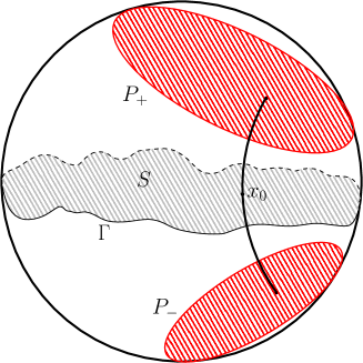
Figure 4.1. The statement of Proposition 4.1. The geodesic segment through $x_{0}$ has length $\leq w$, for $w=\operatorname{arctanh}(2||\Psi||_{\mathcal{B}})$, and this does not depend on $x_{0}\in S$.

Remark 4.2.

A consequence of Proposition 4.1 is that the Hausdorff distance between the two boundary components of $\mathcal{CH}(\Gamma)$ is bounded by $\operatorname{arctanh}(2||\Psi||_{\mathcal{B}})$. Hence it would be natural to try to define in such a way a notion of thickness or width of the convex hull:

$$w(\Gamma)=\max\{\inf_{x\in\partial_{-}\mathcal{CH}(\Gamma)}d(x,\partial_{+}\mathcal{CH}(\Gamma)),\inf_{x\in\partial_{+}\mathcal{CH}(\Gamma)}d(x,\partial_{-}\mathcal{CH}(\Gamma))\}$$

However, a bound on the Hausdorff distance is not sufficient for the purpose of this paper. It will become clear in the proof of Theorem C and Theorem A, and in particular for the application of Lemma 4.15, that the necessary property is the existence of two support planes which are both orthogonal to a geodesic segment of short length through any point $x_{0}\in S$.

We review here some important facts on the so-called description from infinity of surfaces in hyperbolic space. For details, see [Eps84] and [KS08]. Given an embedded surface $S$ in $\mathbb{H}^{3}$ with bounded principal curvatures, let $I$ be its first fundamental form and $II$ the second fundamental form. Recall we defined $B=-\nabla N$ its shape operator, for $N$ the oriented unit normal vector field (we fix the convention that $N$ points towards the $x_{4}>0$ direction in ${\mathbb{R}}^{3,1}$), so that $II=I(B\cdot,\cdot)$. Denote by $E$ the identity operator. Let $S_{\rho}$ be the $\rho$-equidistant surface from $S$ (where the sign of $\rho$ agrees with the choice of unit normal vector field to $S$). For small $\rho$, there is a map from $S$ to $S_{\rho}$ obtained following the geodesics orthogonal to $S$ at every point.

Lemma 4.3.

Given a smooth surface $S$ in $\mathbb{H}^{3}$, let $S_{\rho}$ be the surface at distance $\rho$ from $S$, obtained by following the normal flow at time $\rho$. Then the pull-back to $S$ of the induced metric on the surface $S_{\rho}$ is given by:

(9) $$I_{\rho}=I((\cosh(\rho)E-\sinh(\rho)B)\cdot,(\cosh(\rho)E-\sinh(\rho)B)\cdot)\,.$$

The second fundamental form and the shape operator of $S_{\rho}$ are given by

(10) $$II_{\rho}=I((-\sinh(\rho)E+\cosh(\rho)B)\cdot,(\cosh(\rho)E-\sinh(\rho)B)\cdot)$$

(11) $$B_{\rho}=(\cosh(\rho)E-\sinh(\rho)B)^{-1}(-\sinh(\rho)E+\cosh(\rho)B)\,.$$

Proof.

In the hyperboloid model, let $\sigma:\mathbb{D}\rightarrow\mathbb{H}^{2}$ be the minimal embedding of the surface $S$, with oriented unit normal $N$. The geodesics orthogonal to $S$ at a point $x$ can be written as

$$\gamma_{x}(\rho)=\cosh(\rho)\sigma(x)+\sinh(\rho)N(x)\,.$$

Then we compute

$$I_{\rho}(v,w)= \langle d\gamma_{x}(\rho)(v),d\gamma_{x}(\rho)(w)\rangle$$

$$= \langle\cosh(\rho)d\sigma_{x}(v)+\sinh(\rho)dN_{x}(v),\cosh(r)d\sigma_{x}(w)+\sinh(\rho)dN_{x}(w)\rangle$$

$$= I(\cosh(\rho)v-\sinh(\rho)B(v),\cosh(\rho)w-\sinh(\rho)B(w))\,.$$

The formula for the second fundamental form follows from the fact that $II_{\rho}=-\frac{1}{2}\frac{dI_{\rho}}{d\rho}$. ∎

It follows that, if the principal curvatures of a minimal surface $S$ are $\lambda$ and $-\lambda$, then the principal curvatures of $S_{\rho}$ are

(12) $$\lambda_{\rho}=\frac{\lambda-\tanh(\rho)}{1-\lambda\tanh(\rho)}\qquad\lambda^{\prime}_{\rho}=\frac{-\lambda-\tanh(\rho)}{1+\lambda\tanh(\rho)}\,.$$

In particular, if $-1\leq\lambda\leq 1$, then $I_{\rho}$ is a non-singular metric for every $\rho$. The surfaces $S_{\rho}$ foliate $\mathbb{H}^{3}$ and they all have asymptotic boundary $\partial_{\infty}S_{\rho}=\partial_{\infty}S$.

We now define the first, second and third fundamental form at infinity associated to $S$. Recall the second and third fundamental form of $S$ are $II=I(B\cdot,\cdot)$ and $III=I(B\cdot,B\cdot)$.

(13) $$I^{*}=\lim_{\rho\rightarrow\infty}2e^{-2\rho}I_{\rho}=\frac{1}{2}I((E-B)\cdot,(E-B)\cdot)=\frac{1}{2}(I-2II+III)$$

(14) $$B^{*}=(E-B)^{-1}(E+B)$$

(15) $$II^{*}=\frac{1}{2}I((E+B)\cdot,(E-B)\cdot)=I^{*}(B^{*}\cdot,\cdot)$$

(16) $$III^{*}=I^{*}(B^{*}\cdot,B^{*}\cdot)$$

We observe that the metric $I_{\rho}$ and the second fundamental form can be recovered as

(17) $$I_{\rho}=\frac{1}{2}e^{2\rho}I^{*}+II^{*}+\frac{1}{2}e^{-2\rho}III^{*}$$

(18) $$II_{\rho}=-\frac{1}{2}\frac{dI_{\rho}}{d\rho}=\frac{1}{2}I^{*}((e^{\rho}E+e^{-\rho}B^{*})\cdot,(-e^{\rho}E+e^{-\rho}B^{*})\cdot)$$

(19) $$B_{\rho}=(e^{\rho}E+e^{-\rho}B^{*})^{-1}(-e^{\rho}E+e^{-\rho}B^{*})$$

The following relation can be proved by some easy computation:

Lemma 4.4 ([KS08, Remark 5.4 and 5.5]).

The embedding data at infinity $(I^{*},B^{*})$ associated to an embedded surface $S$ in $\mathbb{H}^{3}$ satisfy the equation

(20) $$tr(B^{*})=-K_{I^{*}}\,,$$

where $K_{I^{*}}$ is the curvature of $I^{*}$. Moreover, $B^{*}$ satisfies the Codazzi equation with respect to $I^{*}$:

(21) $$d^{\nabla_{\!I^{*}}}\!B^{*}=0\,.$$

A partial converse of this fact, which can be regarded as a fundamental theorem from infinity, is the following theorem. This follows again by the results in [KS08], although it is not stated in full generality here.

Theorem 4.5.

Given a Jordan curve $\Gamma\subset\partial_{\infty}\mathbb{H}^{3}$, let $(I^{*},B^{*})$ be a pair of a metric in the conformal class of a connected component of $\partial_{\infty}\mathbb{H}^{3}\setminus\Gamma$ and a self-adjoint $(1,1)$-tensor, satisfiying the conditions (20) and (21) as in Lemma 4.4. Assume the eigenvalues of $B^{*}$ are positive at every point. Then there exists a foliation of $\mathbb{H}^{3}$ by equidistant surfaces $S_{\rho}$, for which the first fundamental form at infinity (with respect to $S=S_{0}$) is $I^{*}$ and the shape operator at infinity is $B^{*}$.

We want to give a relation between the Bers norm of the quasicircle $\Gamma$ and the existence of a foliation of $\mathbb{H}^{3}$ by equidistant surfaces with boundary $\Gamma$, containing both convex and concave surfaces. We identify $\partial_{\infty}\mathbb{H}^{3}$ to $\widehat{\mathbb{C}}$ by means of the stereographic projection, so that $\mathbb{D}$ correponds to the lower hemisphere of the sphere at infinity. The following property will be used, see [ZT87] or [KS08, Appendix A].

Theorem 4.6.

Let $\Gamma\subset\partial_{\infty}\mathbb{H}^{3}$ be a Jordan curve. If $I^{*}$ is the complete hyperbolic metric in the conformal class of a connected component $\Omega$ of $\partial_{\infty}\mathbb{H}^{3}\setminus\Gamma$, and $II_{0}^{*}$ is the traceless part of the second fundamental form at infinity $II^{*}$, then $-II_{0}^{*}$ is the real part of the Schwarzian derivative of the isometry $\Psi:\mathbb{D}^{*}\rightarrow\Omega$, namely the map $\Psi$ which uniformizes the conformal structure of $\Omega$:

(22) $$II_{0}^{*}=-Re(S_{\Psi})\,.$$

We now derive, by straightforward computation, a useful relation.

Lemma 4.7.

Let $\Gamma=\Psi(S^{1})$ be a quasicircle, for $\Psi\in QD(\mathbb{D})$. If $I^{*}$ is the complete hyperbolic metric in the conformal class of a connected component $\Omega$ of $\partial_{\infty}\mathbb{H}^{3}\setminus\Gamma$, and $B_{0}^{*}$ is the traceless part of the shape operator at infinity $B^{*}$, then

(23) $$\sup_{z\in\Omega}|\det B_{0}^{*}(z)|=||\Psi||^{2}_{\mathcal{B}}\,.$$

Proof.

From Theorem 4.6, $B^{*}_{0}$ is the real part of the holomorphic quadratic differential $-S_{\Psi}$. In complex conformal coordinates, we can assume that

$$I^{*}=e^{2\eta}|dz|^{2}=\begin{pmatrix}0&\frac{1}{2}e^{2\eta}\\ \frac{1}{2}e^{2\eta}&0\end{pmatrix}$$

and $S_{\Psi}=h(z)dz^{2}$, so that

$$II_{0}^{*}=-\frac{1}{2}(h(z)dz^{2}+\overline{h(z)}d\bar{z}^{2})=-\begin{pmatrix}\frac{1}{2}h&0\\ 0&\frac{1}{2}\bar{h}\end{pmatrix}$$

and finally

$$B_{0}^{*}=(I^{*})^{-1}II_{0}^{*}=-\begin{pmatrix}0&e^{-2\eta}\bar{h}\\ e^{-2\eta}h&0\end{pmatrix}.$$

Therefore $|\det B_{0}^{*}(z)|=e^{-4\eta(z)}|h(z)|^{2}$. Moreover, by definition of Bers embedding, $\mathcal{B}([{\Psi}])=S_{\Psi}$, because $\Psi$ is a holomorphic map from $\mathbb{D}^{*}$ which maps $S^{1}=\partial\mathbb{D}$ to $\Gamma$. Since

$$||\Psi||_{\mathcal{B}}^{2}=\sup_{z\in\Omega}(e^{-4\eta(z)}|h(z)|^{2})\,,$$

this concludes the proof. ∎

We are finally ready to prove Proposition 4.1.

Proof of Proposition 4.1.

Suppose again $I^{*}$ is a hyperbolic metric in the conformal class of $\Omega$. Since $tr(B^{*})=1$ by Lemma 4.4, we can write $B^{*}=B^{*}_{0}+(1/2)E$, where $B^{*}_{0}$ is the traceless part of $B^{*}$. The symmetric operator $B^{*}$ is diagonalizable; therefore we can suppose its eigenvalues at every point are $(a+1/2)$ and $(-a+1/2)$, where $a$ is a positive number depending on the point. Hence $\pm a$ are the eigenvalues of the traceless part $B_{0}^{*}$.

By using Equation (23) of Lemma 4.7, and observing that $|\det B_{0}^{*}|=a^{2}$, one obtains $||\Psi||_{\mathcal{B}}=||a||_{\infty}$. Since this quantity is less than $A<1/2$ by hypothesis, at every point $a<1/2$, and therefore the eigenvalues of $B^{*}$ are positive at every point.

By Theorem 4.5 there exists a smooth foliation $\mathcal{F}$ of $\mathbb{H}^{3}$ by equidistant surfaces $S_{\rho}$, whose first fundamental form and shape operator are as in equations (17) and (19) above. We are going to compute

$$\rho_{1}=\inf\left\{\rho:B_{\rho}\text{ is non-singular and negative definite}\right\}$$

and

$$\rho_{2}=\sup\left\{\rho:B_{\rho}\text{ is non-singular and positive definite}\right\}.$$

Hence $S_{\rho_{1}}$ is concave and $S_{\rho_{2}}$ is convex. By Corollary 2.5, $S$ is contained in the region bounded by $S_{\rho_{1}}$ and $S_{\rho_{2}}$. We are therefore going to compute $\rho_{1}-\rho_{2}$. From the expression (19), the eigenvalues of $B_{\rho}$ are

$$\lambda_{\rho}=\frac{-2e^{2\rho}+(2a+1)}{2e^{2\rho}+(2a+1)}$$

and

$$\lambda^{\prime}_{\rho}=\frac{-2e^{2\rho}+(1-2a)}{2e^{2\rho}+(1-2a)}.$$

Since $a<1/2$, the denominators of $\lambda_{\rho}$ and $\lambda^{\prime}_{\rho}$ are always positive; one has $\lambda_{\rho}<0$ if and only if $e^{2\rho}>a+1/2$, whereas $\lambda^{\prime}_{\rho}<0$ if and only if $e^{2\rho}>-a+1/2$. Therefore

$$\rho_{1}-\rho_{2}=\frac{1}{2}\left(\log\left(A+\frac{1}{2}\right)-\log\left(-A+\frac{1}{2}\right)\right)=\frac{1}{2}\log\left(\frac{1+2A}{1-2A}\right)=\operatorname{arctanh}(2A)\,.$$

This shows that every point $x$ on $S$ lies on a geodesic orthogonal to the leaves of the foliation, and the distance between the concave surface $S_{\rho_{1}}$ and the convex surface $S_{\rho_{2}}$, on the two sides of $x$, is less than $\operatorname{arctanh}(2A)$. Taking $P_{-}$ and $P_{+}$ the planes tangent to $S_{\rho_{1}}$ and $S_{\rho_{2}}$, the claim is proved. ∎

Remark 4.8.

The proof relies on the observation - given in [KS08] and expressed here implicitly in Theorem 4.5 - that if the shape operator at infinity $B^{*}$ is positive definite, then one reconstructs the shape operator $B_{\rho}$ as in Equation (19), and for $\rho=0$ the principal curvatures are in $(-1,1)$. Hence from our argument it follows that, if the Bers norm $||\Psi||_{\mathcal{B}}$ is less than $1/2$, then one finds a surface $S$ with $\partial_{\infty}S=\Psi(S^{1})$, with principal curvatures in $(-1,1)$. This is a special case of the results in [Eps86], where the existence of such surface is used to prove (using techniques of hyperbolic geometry) a generalization of the univalence criterion of Nehari.

4.2. Boundedness of curvature

Recall that the curvature of a minimal surface $S$ is given by $K_{S}=-1-\lambda^{2}$, where $\pm\lambda$ are the principal curvatures of $S$. We will need to show that the curvature of a complete minimal surface $S$ is also bounded below in a uniform way, depending only on the complexity of $\partial_{\infty}S$. This is the content of Lemma 4.11.

We will use a conformal identification of $S$ with $\mathbb{D}$. Under this identification the metric takes the form $g_{S}=e^{2f}|dz|^{2}$, $|dz|^{2}$ being the Euclidean metric on $\mathbb{D}$. The following uniform bounds on $f$ are known (see [Ahl38]).

Lemma 4.9.

Let $g=e^{2f}|dz|^{2}$ be a conformal metric on $\mathbb{D}$. Suppose the curvature of $g$ is bounded above, $K_{g}<-\epsilon^{2}<0$. Then

(24) $$e^{2f}<\frac{4}{\epsilon^{2}(1-|z|^{2})^{2}}\,.$$

Analogously, if $-\delta^{2}<K_{g}$, then

(25) $$e^{2f}>\frac{4}{\delta^{2}(1-|z|^{2})^{2}}\,.$$

Remark 4.10.

A consequence of Lemma 4.9 is that, for a conformal metric $g=e^{2f}|dz|^{2}$ on $\mathbb{D}$, if the curvature of $g$ is bounded from above by $K_{g}<-\epsilon^{2}<0$, then a conformal ball $B_{0}(p,R)$ (i.e. a ball of radius $R$ for the Euclidean metric $|dz|^{2}$) is contained in the geodesic ball of radius $R^{\prime}$ (for the metric $g$) centered at the same point, where $R^{\prime}$ only depends from $R$. This can be checked by a simple integration argument, and $R^{\prime}$ is actually obtained by multiplying $R$ for the square root of the constant in the RHS of Equation (24). Analogously, a lower bound on the curvature, of the form $-\delta^{2}<K_{g}$, ensures that the geodesic ball of radius $R$ centered at $p$ is contained in the conformal ball $B_{0}(p,R^{\prime})$, where $R^{\prime}$ depends on $R$ and $\delta$.

Lemma 4.11.

For every $K_{0}>1$, there exists a constant $\Lambda_{0}>0$ such that all minimal surfaces $S$ with $\partial_{\infty}S$ a $K$-quasicircle, $K\leq K_{0}$, have principal curvatures bounded by $||\lambda||_{\infty}<\Lambda_{0}$.

We will prove Lemma 4.11 by giving a compactness argument. It is known that a conformal embedding $\sigma:\mathbb{D}\rightarrow\mathbb{H}^{3}$ is harmonic if and only if $\sigma(\mathbb{D})$ is a minimal surface, see [ES64]. The following Lemma is proved in [Cus09] in the more general case of CMC surfaces. We give a sketch of the proof here for convenience of the reader.

Lemma 4.12.

Let $\sigma_{n}:\mathbb{D}\rightarrow\mathbb{H}^{3}$ a sequence of conformal harmonic maps such that $\sigma(0)=x_{0}$ and $\partial_{\infty}(\sigma_{n}(\mathbb{D}))=\Gamma_{n}$ is a Jordan curve, and assume $\Gamma_{n}\rightarrow\Gamma$ in the Hausdoff topology. Then there exists a subsequence $\sigma_{n_{k}}$ which converges $C^{\infty}$ on compact subsets to a conformal harmonic map $\sigma_{\infty}:\mathbb{D}\to\mathbb{H}^{3}$ with $\partial_{\infty}(\sigma_{\infty}(\mathbb{D}))=\Gamma$.

Sketch of proof.

Consider the coordinates on $\mathbb{H}^{3}$ given by the Poincaré model, namely $\mathbb{H}^{3}$ is the unit ball in ${\mathbb{R}}^{3}$. Let $\sigma_{n}^{l}$, for $l=1,2,3$, be the components of $\sigma_{n}$ in such coordinates. Fix $R>0$ for the moment.

Since the curvature of the minimal surfaces $\sigma_{n}(\mathbb{D})$ is less than $-1$, from Lemma 4.9 (setting $\epsilon=1$) and Remark 4.10, for every $n$ we have that $\sigma_{n}(B_{0}(0,2R))$ is contained in a geodesic ball for the induced metric of fixed radius $R^{\prime}$ centered at $x_{0}$. In turn, the geodesic ball for the induced metric is clearly contained in the ball $B_{\mathbb{H}^{3}}(x_{0},R^{\prime})$, for the hyperbolic metric of $\mathbb{H}^{3}$. We remark that the radius $R^{\prime}$ only depends on $R$.

We will apply standard Schauder theory (compare also similar applications in Sections 4.3) to the harmonicity condition

(26) $$\Delta_{0}\sigma_{n}^{l}=-\left(\Gamma_{jk}^{l}\circ\sigma\right)\left(\frac{\partial\sigma_{i}^{j}}{\partial x^{1}}\frac{\partial\sigma_{i}^{k}}{\partial x^{1}}+\frac{\partial\sigma_{i}^{j}}{\partial x^{2}}\frac{\partial\sigma_{i}^{k}}{\partial x^{2}}\right)=:h_{n}^{l}$$

for the Euclidean Laplace operator $\Delta_{0}$, where $\Gamma_{jk}^{l}$ are the Christoffel symbols of the hyperbolic metric in the Poincaré model.

The RHS in Equation (26), which is denoted by $h_{n}^{l}$, is uniformly bounded on $B_{0}(0,2R)$. Indeed Christoffel symbols are uniformly bounded, since $\sigma_{n}(B_{0}(0,2R))$ is contained in a compact subset of $\mathbb{H}^{3}$, as already remarked. The partial derivatives of $\sigma_{n}^{l}$ are bounded too, since one can observe that, if the induced metric on $S$ is $e^{2f}|dz|^{2}$, then $2e^{2f}=||d\sigma||^{2}$, where

$$||d\sigma||^{2}=\frac{4}{(1-\Sigma_{i}(\sigma_{n}^{i})^{2})^{2}}\left(\left(\frac{\partial\sigma_{n}^{1}}{\partial x}\right)^{2}\!\!+\!\left(\frac{\partial\sigma_{n}^{2}}{\partial x}\right)^{2}\!\!+\!\left(\frac{\partial\sigma_{n}^{3}}{\partial x}\right)^{2}\!\!+\!\left(\frac{\partial\sigma_{n}^{1}}{\partial y}\right)^{2}\!\!+\!\left(\frac{\partial\sigma_{n}^{2}}{\partial y}\right)^{2}\!\!+\!\left(\frac{\partial\sigma_{n}^{3}}{\partial y}\right)^{2}\right)\,.$$

Hence from Lemma 4.9 and again the fact that $\sigma_{n}(B_{0}(0,2R))$ is contained in a compact subset of $\mathbb{H}^{3}$, all partial derivatives of $\sigma_{n}$ are uniformly bounded.

The Schauder estimate for the equation $\Delta_{0}\sigma_{n}^{l}=h_{n}^{l}$ ([GT83]) give (for every $\alpha\in(0,1)$) a constant $C_{1}$ such that:

$$||\sigma_{n}^{l}||_{C^{1,\alpha}(B_{0}(0,R_{1}))}\leq C_{1}\left(||\sigma_{n}^{l}||_{C^{0}(B_{0}(0,2R))}+||h_{n}^{l}||_{C^{0}(B_{0}(0,2R))}\right)\,.$$

Hence one obtains uniform $C^{1,\alpha}(B_{0}(0,R_{1}))$ bounds on $\sigma_{n}^{l}$, where $R<R_{1}<2R$, and this provides $C^{0,\alpha}(B_{0}(0,R_{1}))$ bounds on $h_{n}^{l}$. Then the following estimate of Schauder-type

$$||\sigma_{n}^{l}||_{C^{2,\alpha}(B_{0}(0,R_{2}))}\leq C_{2}\left(||\sigma_{n}^{l}||_{C^{0}(B_{0}(0,R_{1}))}+||h_{n}^{l}||_{C^{1,\alpha}(B_{0}(0,R_{1}))}\right)$$

provide $C^{2,\alpha}$ bounds on $B_{0}(0,R_{2})$, for $R<R_{2}<R_{1}$. By a boot-strap argument which repeats this construction, uniform $C^{k,\alpha}(B_{0}(0,R))$ for $\sigma_{n}^{l}$ are obtained for every $k$.

By Ascoli-Arzelà theorem, one can extract a subsequence of $\sigma_{n}$ converging uniformly in $C^{k,\alpha}(B_{0}(0,R))$ for every $k$. By applying a diagonal procedure one can find a subsequence converging $C^{\infty}$. One concludes the proof by a diagonal process again on a sequence of compact subsets $B_{0}(0,R_{n})$ which exhausts $\mathbb{D}$.

The limit function $\sigma_{\infty}:\mathbb{D}\to\mathbb{H}^{3}$ is conformal and harmonic, and thus gives a parametrization of a minimal surface. It remains to show that $\partial_{\infty}(\sigma_{\infty}(\mathbb{D}))=\Gamma$. Since each $\sigma_{n}(\mathbb{D})$ is contained in the convex hull of $\Gamma_{n}$, the Hausdorff convergence on the boundary at infinity ensures that $\sigma_{\infty}(\mathbb{D})$ is contained in the convex hull of $\Gamma$, and thus $\partial_{\infty}(\sigma_{\infty}(\mathbb{D}))\subseteq\Gamma$.

For the other inclusion, assume there exists a point $p\in\Gamma$ which is not in the boundary at infinity of $\sigma_{\infty}(\mathbb{D})$. Then there is a neighborhood of $p$ which does not intersect $\sigma_{\infty}(\mathbb{D})$, and one can find a totally geodesic plane $P$ such that a half-space bounded by $P$ intersects $\Gamma$ (in $p$, for instance), but does not intersect $\sigma_{\infty}(\mathbb{D})$. But such half-space intersects $\sigma_{n}(\mathbb{D})$ for large $n$ and this gives a contradiction. ∎

Proof of Lemma 4.11.

We argue by contradiction. Suppose there exists a sequence of minimal surfaces $S_{n}$ bounded by $K$-quasicircles $\Gamma_{n}$, with $K\leq K_{0}$, with curvature in a point $K_{S_{n}}(x_{n})\leq-n$. Let us consider isometries $T_{n}$ of $\mathbb{H}^{3}$, so that $T_{n}(x_{n})=x_{0}$.

We claim that, since the point $x_{0}$ is contained in the convex hull of $T_{n}(\Gamma_{n})$ for every $n$, the quasicircles $T_{n}(\Gamma_{n})$ can be assumed to be the image of $S^{1}$ under $K_{0}$-quasiconformal maps $\Psi_{n}:\widehat{\mathbb{C}}\to\widehat{\mathbb{C}}$, such that $\Psi_{n}$ maps three points of $S^{1}$ (say $1$, $i$ and $-1$) to points of $T_{n}(\Gamma_{n})$ at uniformly positive distance from one another in the spherical metric (thus satisfying the hypothesis of Theorem 3.2). Indeed, recall that composing a $K_{0}$-quasiconformal map by a conformal map does not change the constant $K_{0}$. Thus it suffices to prove that the quasicircles $T_{n}(\Gamma_{n})=\Psi_{n}(S^{1})$ ($\Psi_{n}$ a $K_{0}$-quasiconformal map) contain three points $u_{n},v_{n},w_{n}$ at uniformly positive distance from one another, and then one can re-parameterize the quasicircle by pre-composing $\Psi_{n}$ with a biholomorphism of $\widehat{\mathbb{C}}$ (which is determined by the image of three points on $S^{1}$) so that $1,i,-1$ are mapped to $u_{n},v_{n},w_{n}$. Moreover, it suffices to prove that the quasicircles $T_{n}(\Gamma_{n})$ contain two points $u_{n},v_{n}$ with distance $d_{S^{2}}(u_{n},v_{n})>2C$, where $C$ is some constant independent from $n$. Indeed, the Jordan curve $T_{n}(\Gamma_{n})$ will then necessarily contain a third point $w_{n}$ such that $d_{S^{2}}(u_{n},w_{n})$ and $d_{S^{2}}(v_{n},w_{n})$ are larger than $C$. The latter claim is easily proved by contradiction: if the statement was not true, then for every integer $j$ there would exists a quasicircle $T_{n_{j}}(\Gamma_{n_{j}})$ which is contained in a ball of radius $1/j$ for the spherical metric on $S^{2}$. But then it is clear that, for large $j$, the convex hull of $T_{n_{j}}(\Gamma_{n_{j}})$ would not contain the fixed point $x_{0}$. See Figure 4.2.

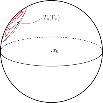
Figure 4.2. If the quasicircle $T_{n}(\Gamma_{n})$ is contained in a small ball for the spherical metric, then the (fixed) point $x_{0}$ cannot be in the convex hull of the quasicircle.

By the compactness property in Theorem 3.2, there exists a subsequence $T_{n_{k}}(\Gamma_{n_{k}})$ converging to a $K$-quasicircle $\Gamma_{\infty}$, with $K\leq K_{0}$. By Lemma 4.12, the minimal surfaces $T_{n_{k}}(S_{n_{k}})$ converge $C^{\infty}$ on compact subsets (up to a subsequence) to a smooth minimal surface $S_{\infty}$ with $\partial_{\infty}(S_{\infty})=\Gamma_{\infty}$. Hence the curvature of $T_{n_{k}}(S_{n_{k}})$ at the point $x_{0}$ converges to the curvature of $S_{\infty}$ at $x_{0}$. This contradicts the assumption that the curvature at the points $x_{n}$ goes to infinity. ∎

It follows that the curvature of $S$ is bounded by $-\delta^{2}<K_{S}<-\epsilon^{2}$, where $\delta$ is some constant, whereas we can take $\epsilon=1$.

Remark 4.13.

The main result of this section, Theorem A, is indeed a quantitative version of Lemma 4.11, which gives a control of how an optimal constant $\Lambda_{0}$ would vary if $K_{0}$ is chosen close to $0$.

4.3. Schauder estimates

By using equation (4), we will eventually obtain bounds on the principal curvatures of $S$. For this purpose, we need bounds on $u=\sinh d_{\mathbb{H}^{3}}(\cdot,P_{-})$ and its derivatives. Schauder theory plays again an important role: since $u$ satisfies the equation

($$\star \Delta_{S}u-2u=0\,.$$ ‣ 2.4)

we will use uniform estimates of the form

$$||u||_{C^{2}(B_{0}(0,\frac{R}{2}))}\leq C||u||_{C^{0}(B_{0}(0,R))}$$

for the function $u$, written in a suitable coordinate system. The main difficulty is basically to show that the operators

$$u\mapsto\Delta_{S}u-2u$$

are strictly elliptic and have uniformly bounded coefficients.

Proposition 4.14.

Let $K_{0}>1$ and $R>0$ be fixed. There exist a constant $C>0$ (only depending on $K_{0}$ and $R$) such that for every choice of:

• A minimal embedded disc $S\subset\mathbb{H}^{3}$ with $\partial_{\infty}S$ a $K$-quasicircle, with $K\leq K_{0}$;

• A point $x\in S$;

• A plane $P_{-}$;

the function $u(\raisebox{-1.07639pt}{\scalebox{1.5}{$\cdot$}})=d_{\mathbb{H}^{3}}(\raisebox{-1.07639pt}{\scalebox{1.5}{$\cdot$}},P_{-})$ expressed in terms of normal coordinates of $S$ centered at $x$, namely

$$u(z)=\sinh d_{\mathbb{H}^{3}}(\exp_{x}(z),P_{-})$$

where $\exp_{x}:{\mathbb{R}}^{2}\cong T_{x}S\rightarrow S$ denotes the exponential map, satisfies the Schauder-type inequality

(27) $$||u||_{C^{2}(B_{0}(0,\frac{R}{2}))}\leq C||u||_{C^{0}(B_{0}(0,R))}\,.$$

Proof.

This will be again an argument by contradiction, using the compactness property.

Suppose our assertion is not true, and find a sequence of minimal surfaces $S_{n}$ with $\partial_{\infty}(S_{n})=\Gamma_{n}$ a $K$-quasicircle ($K\leq K_{0}$), a sequence of points $x_{n}\in S_{n}$, and a sequence of planes $P_{n}$, such that the functions $u_{n}(z)=\sinh d_{\mathbb{H}^{3}}(\exp_{x_{n}}(z),P_{n})$ have the property that

$$||u_{n}||_{C^{2}(B_{0}(0,\frac{R}{2}))}\geq n||u||_{C^{0}(B_{0}(0,R))}\,.$$

We can compose with isometries $T_{n}$ of $\mathbb{H}^{3}$ so that $T_{n}(x_{n})=x_{0}$ for every $n$ and the tangent plane to $T_{n}(S_{n})$ at $x_{0}$ is a fixed plane. Let $S_{n}^{\prime}=T_{n}(S_{n})$, $\Gamma_{n}^{\prime}=T_{n}(\Gamma_{n})$ and $P_{n}^{\prime}=T_{n}(P_{n})$. Note that $\Gamma_{n}^{\prime}$ are again $K$-quasicircles, for $K\leq K_{0}$, and the convex hull of each $\Gamma_{n}^{\prime}$ contains $x_{0}$.

Using this fact, it is then easy to see - as in the proof of Lemma 4.11 - that one can find $K_{0}$-quasiconformal maps $\Psi_{n}$ such that $\Psi_{n}(S^{1})=\Gamma_{n}^{\prime}$ and $\Psi_{n}(1)$, $\Psi_{n}(i)$ and $\Psi_{n}(-1)$ are at uniformly positive distance from one another. Therefore, using Theorem 3.2 there exists a subsequence of $\Psi_{n}$ converging uniformly to a $K_{0}$-quasiconformal map. This gives a subsequence $\Gamma_{n_{k}}^{\prime}$ converging to $\Gamma_{\infty}^{\prime}$ in the Hausdorff topology.

By Lemma 4.12, considering $S_{n}^{\prime}$ as images of conformal harmonic embeddings $\sigma_{n}^{\prime}:\mathbb{D}\rightarrow\mathbb{H}^{3}$, we find a subsequence of $\sigma_{n_{k}}^{\prime}$ converging $C^{\infty}$ on compact subsets to the conformal harmonic embedding of a minimal surface $S_{\infty}^{\prime}$. Moreover, by Lemma 4.11 and Remark 4.10, the convergence is also $C^{\infty}$ on the image under the exponential map of compact subsets containing the origin of ${\mathbb{R}}^{2}$.

It follows that the coefficients of the Laplace-Beltrami operators $\Delta_{S_{n}^{\prime}}$ on a Euclidean ball $B_{0}(0,R)$ of the tangent plane at $x_{0}$, for the coordinates given by the exponential map, converge to the coefficients of $\Delta_{S_{\infty}^{\prime}}$. Therefore the operators $\Delta_{S_{n}^{\prime}}-2$ are uniformly strictly elliptic with uniformly bounded coefficients. Using these two facts, one can apply Schauder estimates to the functions $u_{n}$, which are solutions of the equations $\Delta_{S_{n}^{\prime}}(u_{n})-2u_{n}=0$. See again [GT83] for a reference. We deduce that there exists a constant $c$ such that

$$||u_{n}||_{C^{2}(B_{0}(0,\frac{R}{2}))}\leq c||u_{n}||_{C^{0}(B_{0}(0,R))}$$

for all $n$, and this gives a contradiction. ∎

4.4. Principal curvatures

We can now proceed to complete the proof of Theorem A. Fix some $w>0$. We know from Section 4.1 that if the Bers norm is smaller than the constant $(1/2)\tanh(w)$, then every point $x$ on $S$ lies on a geodesic segment $l$ orthogonal to two planes $P_{-}$ and $P_{+}$ at distance $d_{\mathbb{H}^{3}}(P_{-},P_{+})<w$. Obviously the distance is achieved along $l$.

Fix a point $x\in S$. Denote again $u=\sinh d_{\mathbb{H}^{3}}(\cdot,P_{-})$. By Proposition 4.14, first and second partial derivatives of $u$ in normal coordinates on a geodesic ball $B_{S}(x,R/2)$ of fixed radius $R/2$ are bounded by $C||u||_{C^{0}(B_{S}(x,R))}$. The last step for the proof is an estimate of the latter quantity in terms of $w$.

We first need a simple lemma which controls the distance of points in two parallel planes, close to the common orthogonal geodesic. Compare Figure 4.3.

Lemma 4.15.

Let $p\in P_{-}$, $q\in P_{+}$ be the endpoints of a geodesic segment $l$ orthogonal to $P_{-}$ and $P_{+}$ of length $w$. Let $p^{\prime}\in P_{-}$ a point at distance $r$ from $p$ and let $d=d_{\mathbb{H}^{3}}((\pi|_{P_{+}})^{-1}(p^{\prime}),P_{-})$. Then

(28) $$\tanh d=\cosh r\tanh w$$

(29) $$\sinh d=\cosh r\frac{\sinh w}{\sqrt{1-(\sinh r)^{2}(\sinh w)^{2}}}\,.$$

Proof.

This is easy hyperbolic trigonometry, which can actually be reduced to a 2-dimensional problem. However, we give a short proof for convenience of the reader. In the hyperboloid model, we can assume $P_{-}$ is the plane $x_{3}=0$, $p=(0,0,0,1)$ and the geodesic $l$ is given by $l(t)=(0,0,\sinh t,\cosh t)$. Hence $P_{+}$ is the plane orthogonal to $l^{\prime}(w)=(0,0,\cosh w,\sinh w)$ passing through $l(w)=(0,0,\sinh w,\cosh w)$. The point $p^{\prime}$ has coordinates

$$p^{\prime}=(\cos\theta\sinh r,\sin\theta\sinh r,0,\cosh r)$$

and the geodesic $l_{1}$ orthogonal to $P_{-}$ through $p^{\prime}$ is given by

$$l_{1}(d)=(\cosh d)(p^{\prime})+(\sinh d)(0,0,1,0)\,.$$

We have $l_{1}(d)\in P_{+}$ if and only if $\langle l_{1}(d),l^{\prime}(w)\rangle=0$, which is satisfied for

$$\tanh d=\cosh r\tanh w\,,$$

provided $\cosh r\tanh w<1$. The second expression follows straightforwardly. ∎

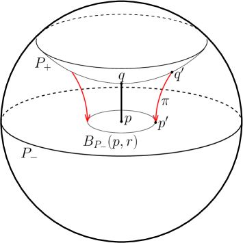
Figure 4.3. The setting of Lemma 4.15. Here $d_{\mathbb{H}^{3}}(p,p^{\prime})=r$ and $q^{\prime}=(\pi|_{P_{+}})^{-1}(p^{\prime})$.

We are finally ready to prove Theorem C. The key point for the proof is that all the quantitative estimates previously obtained in this section are independent on the point $x\in S$.

Theorem C.

There exist constants $K_{0}>1$ and $C>4$ such that the principal curvatures $\pm\lambda$ of every minimal surface $S$ in $\mathbb{H}^{3}$ with $\partial_{\infty}S=\Gamma$ a $K$-quasicircle, with $K\leq K_{0}$, are bounded by:

(30) $$||\lambda||_{\infty}\leq\frac{C||\Psi||_{\mathcal{B}}}{\sqrt{1-C||\Psi||_{\mathcal{B}}^{2}}}$$

where $\Gamma=\Psi(S^{1})$, for $\Psi\in QD(\mathbb{D})$.

Proof.

Fix $K_{0}>1$. Let $S$ a minimal surface with $\partial_{\infty}S$ a $K$-quasicircle, $K\leq K_{0}$. Let $x\in S$ an arbitrary point on a minimal surface $S$. By Proposition 4.1, we find two planes $P_{-}$ and $P_{+}$ whose common orthogonal geodesic passes through $x$, and has length $w=\operatorname{arctanh}(2||\Psi||_{\mathcal{B}})$.

Now fix $R>0$. By Proposition 4.14, applied to the point $x$ and the plane $P_{-}$, we obtain that the first and second derivatives of the function

$$u=\sinh d_{\mathbb{H}^{3}}(\exp_{x}(\raisebox{-1.07639pt}{\scalebox{1.5}{$\cdot$}}),P_{-})$$

on a geodesic ball $B_{S}(x,R/2)$ for the induced metric on $S$, are bounded by the supremum of $u$ itself, on the geodesic ball $B_{S}(x,R)$, multiplied by a universal constant $C=C(K_{0},R)$.

Let $\pi:\mathbb{H}^{3}\rightarrow P_{-}$ the orthogonal projection to the plane $P_{-}$. The map $\pi$ is contracting distances, by negative curvature in the ambient manifold. Hence $\pi(B_{S}(x,R))$ is contained in $B_{P_{-}}(\pi(x),R)$. Moreover, since $S$ is contained in the region bounded by $P_{-}$ and $P_{+}$, clearly $\sup\{u(x):x\in B_{S}(0,R)\}$ is less than the hyperbolic sine of the distance of points in $(\pi|_{P_{+}})^{-1}(B_{P_{-}}(\pi(x),R))$ from $P_{-}$. See Figure 4.4.

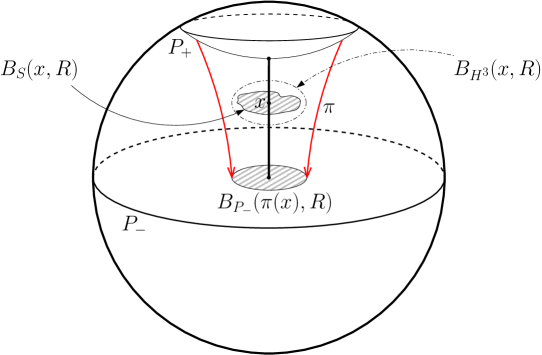
Figure 4.4. Projection to a plane $P_{-}$ in $\mathbb{H}^{3}$ is distance contracting. The dash-dotted ball schematically represents a geodesic ball of $\mathbb{H}^{3}$.

Hence, using Proposition 4.15 (in particular Equation (29)), we get:

(31) $$||u||_{C^{0}(B_{S}(x,R))}\leq\cosh R\frac{\sinh w}{\sqrt{1-(\sinh R)^{2}(\sinh w)^{2}}}\,,$$

where we recall that $w=\operatorname{arctanh}(2||\Psi||_{\mathcal{B}})$.

We finally give estimates on the principal curvatures of $S$, in terms of the complexity of $\partial_{\infty}(S)=\Psi(S^{1})$. We compute such estimate only at the point $x\in S$; by the independence of all the above construction from the choice of $x$, the proof will be concluded. From Equation (4), we have

$$B=\frac{1}{\sqrt{1+u^{2}-||\operatorname{grad}u||^{2}}}(\mathrm{Hess}\,u-u\,E)\,.$$

Moreover, in normal coordinates centered at the point $x$, the expression for the Hessian and the norm of the gradient at $x$ are just

$$(\mathrm{Hess}u)_{i}^{j}=\frac{\partial^{2}u}{\partial x^{i}\partial x^{j}}\,,\qquad\qquad||\operatorname{grad}u||^{2}=\left(\frac{\partial u}{\partial x^{1}}\right)^{2}+\left(\frac{\partial u}{\partial x^{2}}\right)^{2}\,.$$

It then turns out that the principal curvatures $\pm\lambda$ of $S$, i.e. the eigenvalues of $B$, are bounded by

(32) $$|\lambda|\leq\frac{C_{1}||u||_{C^{0}(B_{S}(x,R))}}{\sqrt{1-C_{1}||u||_{C^{0}(B_{S}(x,R))}^{2}}}\,.$$

The constant $C_{1}$ involves the constant $C$ of Equation (27) in the statement of Proposition 4.14. Substituting Equation (31) into Equation (32), with some manipulation one obtains

(33) $$||\lambda||_{\infty}\leq\frac{C_{1}(\cosh R)(\tanh w)}{\sqrt{1-(1+C_{1})(\cosh R)^{2}(\tanh w)^{2}}}\,.$$

On the other hand $\tanh w=2||\Psi||_{\mathcal{B}}$. Upon relabelling $C$ with a larger constant, the inequality

$$||\lambda||_{\infty}\leq\frac{C||\Psi||_{\mathcal{B}}}{\sqrt{1-C||\Psi||_{\mathcal{B}}^{2}}}$$

is obtained. ∎

Remark 4.16.

Actually, the statement of Theorem C is true for any choice of $K_{0}>1$ (and the constant $C$ varies accordingly with the choice of $K_{0}$). However, the estimate in Equation (30) does not make sense when $||\Psi||^{2}\geq 1/C$. Indeed, our procedure seems to be quite uneffective when the quasicircle at infinity is “far” from being a circle - in the sense of universal Teichmüller space. Applying Theorem 3.4, this possibility is easily ruled out, by replacing $K_{0}$ in the statement of Theorem C with a smaller constant.

Observe that the function $x\mapsto Cx/\sqrt{1-Cx^{2}}$ is differentiable with derivative $C$ at $x=0$. As a consequence of Theorem 3.4, there exists a constant $L$ (with respect to the statement of Theorem 3.4 above, $L=1/b_{1}$) such that $||\Psi||_{\mathcal{B}}\leq Ld_{\mathcal{T}}([\Psi],[\mathrm{id}])$ if $d_{\mathcal{T}}([\Psi],[\mathrm{id}])\leq r$ for some small radius $r$. Then the proof of Theorem A follows, replacing the constant $C$ by a larger constant if necessary.

Theorem A.

There exist universal constants $K_{0}$ and $C$ such that every minimal embedded disc in $\mathbb{H}^{3}$ with boundary at infinity a $K$-quasicircle $\Gamma\subset\partial_{\infty}\mathbb{H}^{3}$, with $K\leq K_{0}$, has principal curvatures bounded by

$$||\lambda||_{\infty}\leq C\log K\,.$$

Remark 4.17.

With the techniques used in this paper, it seems difficult to give explicit estimates for the best possible value of the constant $C$ of Theorem A. Indeed, in the proof of Theorem C, the constant which occurs in the inequality (30) depends on the choices of the bound $K_{0}$ on the maximal dilatation of the quasicircle, and on the choice of a radius $R$. The radius $R$ does not really have a key role in the proof, since the estimate on the principal curvatures is then used only for the point $x$ (in a manner which does not depend on $x$). However, the choice of $R$ is essentially due to the form of Schauder estimates, which provide a constant $C_{\mathrm{Sch}}$ such that

$$||u||_{C^{2}(B_{0}(0,\frac{R}{2}))}\leq C_{\mathrm{Sch}}||u||_{C^{0}(B_{0}(0,R))}\,,$$

where $C_{\mathrm{Sch}}$ depends on the radius $R$. Moreover, $C_{\mathrm{Sch}}$ depends on the bounds on the coefficient of the equation satisfied by $u$, which in our case is

($$\star \Delta_{S}u-2u=0\,.$$ ‣ 2.4)

The bound on the coefficients of such equation, which depends on the Laplace-Beltrami operator of the minimal surface $S$, thus depends implicitly on the choice of $K_{0}$ (a compactness argument was used in this paper, in the proof of Proposition 4.14). Finally, the dependence on the constant $K_{0}$ appears again in the proof of Theorem A, when applying the fact that the Bers embedding is locally bi-Lipschitz (Theorem 3.4). In fact, the local bi-Lipschitz constant depends on the chosen neighborhood of the identity in universal Teichmüller space.

5. Some applications and open questions

In this section we discuss the proofs of Theorem B, of Corollaries A, B and C, and mention some related questions.

5.1. Uniqueness of minimal discs

We recall here Theorem B, which was stated in the introduction.

Theorem B.

There exists a universal constant $K^{\prime}_{0}$ such that every $K$-quasicircle $\Gamma\subset\partial_{\infty}\mathbb{H}^{3}$ with $K\leq K^{\prime}_{0}$ is the boundary at infinity of a unique minimal embedded disc.

To prove Theorem B, one applies the well-known fact that a minimal disc in $\mathbb{H}^{3}$ with principal curvatures in $[-1+\epsilon,1-\epsilon]$ for some $\epsilon>0$ is the unique one with fixed boundary at infinity. Under this hypothesis, the curve at infinity is necessarily a quasicircle (one can adapt the argument of [GHW10, Lemma 3.3]). For the convenience of the reader, we provide here a sketch of a proof which uses the tools of this paper.

Lemma 5.1.

Let $S$ be a minimal embedded disc in $\mathbb{H}^{3}$ with $\partial_{\infty}S=\Gamma$. If the principal curvatures of $S$ satisfy $||\lambda||_{\infty}<1$, then $S$ is the unique minimal disc with $\partial_{\infty}S=\Gamma$.

Sketch of proof.

Suppose $\Gamma$ is such that there exists two minimal surfaces $S$ and $S^{\prime}$ with $\partial_{\infty}S=\partial_{\infty}S^{\prime}=\Gamma$, and that the principal curvatures of $S$ are in $[-1+\epsilon,1-\epsilon]$. As observed after the proof of Lemma 4.3, the $\rho$-equidistant surfaces from $S$ give a foliation of a convex subset $\mathcal{C}$ of $\mathbb{H}^{3}$, for $\rho\in(-\operatorname{arctanh}||\lambda||_{\infty},\operatorname{arctanh}||\lambda||_{\infty})$. By Corollary 2.5, the minimal surface $S^{\prime}$ is also contained in $\mathcal{C}$.

Now, let $\rho_{0}$ the supremum of the value of $\rho$ on the minimal surface $S^{\prime}$. If this supremum is achieved on $S^{\prime}$, then the minimal surface $S^{\prime}$ is tangent to the smooth surface $S_{\rho_{0}}$ at distance $\rho_{0}$ from $S$. But by Equation (12), when $\rho>0$ the mean curvature of $S_{\rho}$ is negative (in our setting, a concave surface, for instance obtained for large positive $\rho$, has negative principal curvatures). Hence by the maximum principle, necessarily $\rho_{0}\leq 0$.

If the supremum is not attained, let us pick a sequence of points $x_{n}\in S^{\prime}$ such that the value of $\rho$ at $x_{n}$ converges to $\rho_{0}$ as $n\to\infty$. One can apply isometries $T_{n}$ of $\mathbb{H}^{3}$ so that $x_{n}$ is mapped to a fixed point $x_{0}$. By the usual argument (see also Lemma 4.11), one can apply Theorem 3.2 to ensure that the quasicircles $T_{n}(\Gamma)$ converge to a quasicircle $\Gamma_{\infty}$, and then Lemma 4.12 to get the $C^{\infty}$ convergence on compact sets of the minimal discs $T_{n}(S^{\prime})$ to a minimal disc $S^{\prime}_{\infty}$ with $\partial_{\infty}S^{\prime}_{\infty}=\Gamma_{\infty}$, up to a subsequence. Moreover, one can also assume that the minimal discs $T_{n}(S)$ converge to a minimal disc $S_{\infty}$. Indeed, consider the points $y_{n}$ on $S$ such that the geodesic of $\mathbb{H}^{3}$ through $y_{n}$, perpendicular to $S$, contains $x_{n}$. The isometries $T_{n}$ map $y_{n}$ to a compact region of $y_{n}$ (as $d(x_{0},T_{n}(y_{n}))=d(x_{n},y_{n})\leq\operatorname{arctanh}||\lambda||_{\infty}$), thus one can repeat the previous argument (first compose with isometries $R_{n}$ which map $T_{n}(y_{n})$ to a fixed point $y_{0}$, and extract a subsequence of $R_{n}$ converging to an isometry $R_{\infty}$). By the $C^{\infty}$ convergence, the minimal surface $S_{\infty}$ still has principal curvatures in $[-1+\epsilon,1-\epsilon]$, and therefore one can repeat the argument of the previous paragraph, applied to $S_{\infty}$ and $S^{\prime}_{\infty}$, to show that $\rho_{0}\leq 0$.

In the same way, one proves that the infimum of $\rho$ on $S^{\prime}$ must be nonnegative, and thus $\rho$ must always be zero on $S^{\prime}$. This proves that $S=S^{\prime}$. ∎

The proof of Theorem B then follows from Lemma 5.1. With respect to the constants $K_{0}$ and $C$ of Theorem A, by choosing some constant $K_{0}^{\prime}<\min\{K_{0},e^{1/C}\}$ one obtains that every minimal embedded disc with boundary at infinity a $K$-quasicircle, with $K\leq K_{0}^{\prime}$, has principal curvatures bounded by $||\lambda||_{\infty}<1$.

5.2. Quasi-Fuchsian manifolds

In this subsection we collect the applications of Theorem A to quasi-Fuchsian manifolds. A quasi-Fuchsian manifold is a Riemannian manifold isometric to $\mathbb{H}^{3}/G$, where $G$ is subgroup of $\mathrm{Isom}(\mathbb{H}^{3})$, which acts freely and properly discontinuously on $\mathbb{H}^{3}$, isomorphic to the fundamental group of a closed surface $\Sigma$, and such that the limit set (i.e. the set of accumulation points in $\partial_{\infty}\mathbb{H}^{3}$ of orbits of the action of $G$) is a quasicircle. The topology of a quasi-Fuchsian manifold is $\Sigma\times{\mathbb{R}}$, where $\Sigma$ is the closed surface. Therefore the results obtained in the previous sections hold for the universal cover $S=\tilde{\Sigma}_{0}$ of any closed minimal surface $\Sigma_{0}$ homotopic to $\Sigma\times\{0\}$.

Recall that Teichmüller space $\mathcal{T}(\Sigma)$ of a closed surface $\Sigma$ is the space of Riemann surface structures on $\Sigma$, considered up to biholomorphisms isotopic to the identity. In the same way, the classifying space for quasi-Fuchsian manifolds, which we denote by $\mathcal{QF}(\Sigma)$, is the space of quasi-Fuchsian metrics on $\Sigma\times{\mathbb{R}}$ up to isometries isotopic to the identity. By the celebrated Bers’ Simultaneous Uniformization Theorem ([Ber60]), $\mathcal{QF}(\Sigma)$ is parameterized by $\mathcal{T}(\Sigma)\times\mathcal{T}(\Sigma)$. The construction is as follows: since the limit set $\Lambda$ of $G$ is a Jordan curve, the complement of $\Lambda$ in $\partial_{\infty}\mathbb{H}^{3}$ has two connected components $\Omega_{+}$ and $\Omega_{-}$ on which $G$ acts freely, properly discontinuously and by biholomorphisms. This construction thus provides two Riemann surface structures on $\Sigma$, namely the structures given by the quotients $\Omega_{+}/G$ and $\Omega_{-}/G$. Bers proved that these two Riemann surface structures, as points in $\mathcal{T}(\Sigma)$, can be prescribed and determine uniquely the quasi-Fuchsian structure in $\mathcal{QF}(\Sigma)$.

Finally, recall that the Teichmüller distance between two points of $\mathcal{T}(\Sigma)$, namely two Riemann surface structures $\mathcal{A}_{1}$ and $\mathcal{A}_{2}$ on $\Sigma$, is defined as:

$$d_{\mathcal{T}(\Sigma)}((\Sigma,\mathcal{A}_{1}),(\Sigma,\mathcal{A}_{2}))=\frac{1}{2}\inf_{f\sim\mathrm{id}}\log K(f)\,,$$

where $K(f)$ is the maximal dilatation of $f$ and the infimum is taken over all $f:(\Sigma,\mathcal{A}_{1})\to(\Sigma,\mathcal{A}_{2})$ quasiconformal and isotopic to the identity.

Corollary A.

There exist universal constants $C>0$ and $d_{0}>0$ such that, for every quasi-Fuchsian manifold $M=\mathbb{H}^{3}/G$ with $d_{\mathcal{T}(\Sigma)}(\Omega_{+}/G,\Omega_{-}/G)<d_{0}$ and every minimal surface $S$ in $M$ homotopic to $\Sigma\times\{0\}$, the supremum of the principal curvatures of $S$ satisfies:

$$||\lambda||_{\infty}\leq Cd_{\mathcal{T}(\Sigma)}(\Omega_{+}/G,\Omega_{-}/G)\,.$$

Corollary A follows directly from Theorem A. Indeed, let us choose $d_{0}=(1/2)\log K_{0}$. If the Teichmüller distance between $\Omega_{+}/G$ and $\Omega_{-}/G$ is less than $d_{0}$, then for every $d<d_{0}$, $d$ larger than the Teichmüller distance, one can obtain (by lifting to the universal cover) a $K$-quasiconformal map between $\Omega_{+}$ and $\Omega_{-}$ with $K=e^{2d}\leq K_{0}$. Thus the limit set $\Gamma$ is a $K$-quasicircle, with $K\leq K_{0}$. Thus by Theorem A the lift $S=\tilde{\Sigma}_{0}$ of any minimal surface in $M$ satisfies

$$||\lambda||_{\infty}\leq C\log K=2Cd$$

Since the choice of $d$ was arbitrary, one obtains

$$||\lambda||_{\infty}\leq 2Cd_{\mathcal{T}(\Sigma)}(\Omega_{+}/G,\Omega_{-}/G)$$

and the statement is concluded, replacing $C$ by $2C$.

Clearly, the simplest example of quasi-Fuchsian manifolds are Fuchsian manifolds, namely those quasi-Fuchsian manifolds which contain a totally geodesic (and thus minimal) surface homotopic to $\Sigma\times\{0\}$. The lift to $\mathbb{H}^{3}$ of such surface is a totally geodesic plane, whose boundary at infinity is a circle. Fuchsian manifolds are parameterized by the induced metric on this totally geodesic surface, and thus the space $\mathcal{F}$ of Fuchsian metrics on $\Sigma\times{\mathbb{R}}$, up to isometry isotopic to the identity, is parameterized by $\mathcal{T}(\Sigma)$. As a subset of $\mathcal{QF}$, $\mathcal{F}$ is precisely the diagonal in $\mathcal{T}(\Sigma)\times\mathcal{T}(\Sigma)$.

It is easy to see that the totally geodesic surface in a quasi-Fuchsian manifold is the unique minimal surface. Although the uniqueness of the minimal surface in a quasi-Fuchsian manifold does not hold in general, there is a larger class of manifolds where uniqueness is guaranteed. According to the terminology in [KS07], we have the following definition of almost-Fuchsian manifolds:

Definition 5.2.

A quasi-Fuchsian manifold is almost-Fuchsian if it contains a minimal surface homotopic to $\Sigma\times\{0\}$ with principal curvatures in $(-1,1)$.

We will denote by $\mathcal{AF}(\Sigma)$ the subset of $\mathcal{QF}(\Sigma)$ of almost-Fuchsian manifolds. Uhlenbeck in [Uhl83] first observed that the minimal surface in an almost-Fuchsian manifold is unique. This follows also from the proof of Lemma 5.1, in a simplified version for the compact case. A direct consequence of our results is the following:

Corollary B.

If the Teichmüller distance between the conformal metrics at infinity of a quasi-Fuchsian manifold $M$ is smaller than a universal constant $d_{0}^{\prime}$, then $M$ is almost-Fuchsian.

Indeed, in Corollary A, if the Teichmüller distance is small enough, then the principal curvatures are bounded by $1$ in absolute value. Finally, if we endow $\mathcal{QF}\cong\mathcal{T}(\Sigma)\times\mathcal{T}(\Sigma)$ by the 1-product metric, namely

$$d_{\mathcal{T}(\Sigma)\times\mathcal{T}(\Sigma)}((\mathcal{A}_{1},\mathcal{A}^{\prime}_{1}),(\mathcal{A}_{2},\mathcal{A}^{\prime}_{2}))=d_{\mathcal{T}(\Sigma)}(\mathcal{A}_{1},\mathcal{A}_{2})+d_{\mathcal{T}(\Sigma)}(\mathcal{A}^{\prime}_{1},\mathcal{A}^{\prime}_{2})\,,$$

then Corollary B can be restated by saying that if the distance of a point $(\Omega_{+}/G,\Omega_{-}/G)$ from the diagonal is less than $d_{0}^{\prime}$, then the quasi-Fuchsian manifold determined by $(\Omega_{+}/G,\Omega_{-}/G)$ is almost-Fuchsian. We state this in Corollary C below.

Corollary C.

There exists a uniform neighborhood $N(\mathcal{F}(\Sigma))$ of the Fuchsian locus $\mathcal{F}(\Sigma)$ in $\mathcal{QF}(\Sigma)\cong\mathcal{T}(\Sigma)\times\mathcal{T}(\Sigma)$ such that $N(\mathcal{F}(\Sigma))\subset\mathcal{AF}(\Sigma)$.

5.3. Further directions

There is a number of questions left open on quasi-Fuchsian and almost-Fuchsian manifolds. In particular, the results presented in this paper hold for quasi-Fuchsian manifolds such that the two Riemann surfaces at infinity are close in Teichmüller space. The understanding of the subset of almost-Fuchsian manifolds far from the Fuchsian locus is far from being completed. More in general, it is an interesting and challenging problem to understand the geometric behavior of minimal discs in hyperbolic space with boundary at infinity a Jordan curve, especially when this Jordan curve becomes more exotic and phenomena of bifurcations occur.

The techniques of this paper, as observed in Remark 4.2, motivate towards a definition of thickness or width of the convex core of a quasi-Fuchsian manifold or, more in general, the convex hull of a quasicircle in $\partial_{\infty}\mathbb{H}^{3}$. One might expect to find a relation between such notion of thickness and, for instance, the Teichmüller distance between the conformal ends of the quasi-Fuchsian manifold, or the maximal dilatation of the quasicircle. Again, it seems challenging to provide relations which hold far from the Fuchsian locus.

References

- [Ahl38] L. V. Ahlfors. An extension of Schwarz’s lemma. Trans. Amer. Math. Soc., 43:359–364, 1938.
- [Ahl06] Lars V. Ahlfors. Lectures on quasiconformal mappings, volume 38 of University Lecture Series. American Mathematical Society, Providence, RI, second edition, 2006. With supplemental chapters by C. J. Earle, I. Kra, M. Shishikura and J. H. Hubbard.
- [And83] Michael T. Anderson. Complete minimal hypersurfaces in hyperbolic -manifolds. Comment. Math. Helv., 58(2):264–290, 1983.
- [Ber60] Lipman Bers. Simultaneous uniformization. Bull. Amer. Math. Soc., 66:94–97, 1960.
- [Cos13] Baris Coskunuzer. Asymptotic plateau problem. In Proc. Gokova Geom. Top. Conf., pages 120–146, 2013.
- [Cus09] Thomas Cuschieri. Complete Noncompact CMC Surfaces in Hyperbolic 3-Space. PhD thesis, University of Warwick, 2009.
- [Eps84] Charles L. Epstein. Envelopes of horospheres and Weingarten surfaces in hyperbolic 3-space. Princeton Univ, 1984.
- [Eps86] Charles L. Epstein. The hyperbolic Gauss map and quasiconformal reflections. J. Reine Angew. Math., 372:96–135, 1986.
- [ES64] J. Eells and J.H. Sampson. Harmonic mappings of Riemannian manifolds. Amer. J. Math, 86:109–159, 1964.
- [FKM13] Alastair Fletcher, Jeremy Kahn, and Vladimir Markovic. The moduli space of Riemann surfaces of large genus. Geom. Funct. Anal., 23(3):867–887, 2013.
- [FM07] A. Fletcher and V. Markovic. Quasiconformal maps and Teichmüller theory, volume 11 of Oxford Graduate Texts in Mathematics. Oxford University Press, Oxford, 2007.
- [Gar87] F. P. Gardiner. Teichmüller theory and quadratic differentials. Wiley, 1987.
- [GHW10] Ren Guo, Zheng Huang, and Biao Wang. Quasi-Fuchsian 3-manifolds and metrics on Teichmüller space. Asian J. Math., 14(2):243–256, 2010.
- [GL00] F. P. Gardiner and N. Lakic. Quasiconformal Teichmüller Theory. American Mathematical Soc., 2000.
- [GT83] David Gilbarg and Neil S. Trudinger. Elliptic partial differential equations of second order, volume 224 of Grundlehren der Mathematischen Wissenschaften [Fundamental Principles of Mathematical Sciences]. Springer-Verlag, Berlin, second edition, 1983.
- [HW13a] Zheng Huang and Biao Wang. Counting minimal surfaces in quasi-fuchsian manifolds. To appear in Trans. Amer. Math. Soc., 2013.
- [HW13b] Zheng Huang and Biao Wang. On almost-Fuchsian manifolds. Trans. Amer. Math. Soc., 365(9):4679–4698, 2013.
- [KS07] Kirill Krasnov and Jean-Marc Schlenker. Minimal surfaces and particles in 3-manifolds. Geom. Dedicata, 126:187–254, 2007.
- [KS08] Kirill Krasnov and Jean-Marc Schlenker. On the renormalized volume of hyperbolic 3-manifolds. Comm. Math. Phys., 279(3):637–668, 2008.
- [Leh87] O. Lehto. Univalent functions and Teichmüller spaces. Springer Verlag, Berlin 1987.
- [San13] Andrew Sanders. Domains of discontinuity for almost-Fuchsian groups. To appear on Trans. Amer. Math. Soc., 2013. ArXiv: 1310.6412.
- [San14] Andrew Sanders. Entropy, minimal surfaces, and negatively curved manifolds. Arxiv: 1404.1105, 2014.
- [Sug07] Toshiyuki Sugawa. The universal Teichmüller space and related topics. In Quasiconformal mappings and their applications, pages 261–289. Narosa, New Delhi, 2007.
- [Uhl83] Karen K. Uhlenbeck. Closed minimal surfaces in hyperbolic -manifolds. In Seminar on minimal submanifolds, volume 103 of Ann. of Math. Stud., pages 147–168. Princeton Univ. Press, Princeton, NJ, 1983.
- [ZT87] P. G. Zograf and L. A. Takhtadzhyan. On the uniformization of Riemann surfaces and on the Weil-Petersson metric on the Teichmüller and Schottky spaces. Mat. Sb. (N.S.), 132(174)(3):304–321, 444, 1987.