Multi-view Anomaly Detection
via Probabilistic Latent Variable Models

Abstract

We propose a nonparametric Bayesian probabilistic latent variable model for multi-view anomaly detection, which is the task of finding instances that have inconsistent views. With the proposed model, all views of a non-anomalous instance are assumed to be generated from a single latent vector. On the other hand, an anomalous instance is assumed to have multiple latent vectors, and its different views are generated from different latent vectors. By inferring the number of latent vectors used for each instance with Dirichlet process priors, we obtain multi-view anomaly scores. The proposed model can be seen as a robust extension of probabilistic canonical correlation analysis for noisy multi-view data. We present Bayesian inference procedures for the proposed model based on a stochastic EM algorithm. The effectiveness of the proposed model is demonstrated in terms of performance when detecting multi-view anomalies and imputing missing values in multi-view data with anomalies.

1 Introduction

There has been great interest in multi-view learning, in which data are obtained from various information sources (Blum and Mitchell, 1998; Bickel and Scheffer, 2004; Sindhwani and Rosenberg, 2008). In a wide variety of applications, data are naturally comprised of multiple views. For example, an image can be represented by color, texture and shape information; a web page can be represented by words, images and URLs occurring on in the page; and a video can be represented by audio and visual features. In this paper, we consider the task of finding anomalies in multi-view data. The task is called horizontal anomaly detection (Gao et al, 2011), or multi-view anomaly detection (Liu and Lam, 2012). Anomalies in multi-view data are instances that have inconsistent features across multiple views. Multi-view anomaly detection is different from standard (single-view) anomaly detection. Single-view anomaly detection finds instances that do not conform to expected behavior (Chandola et al, 2009).

Figure 1 (a,b) shows the difference between a multi-view anomaly and a single-view anomaly in a two-view data set. ‘M’ is a multi-view anomaly since ‘M’ belongs to different clusters in different views (‘A–D’ cluster in View 1 and ‘E–J’ cluster in View 2) and views of ‘M’ are not consistent. ‘S’ is a single-view anomaly since ‘S’ is located far from other instances in each view. However, both views of ‘S’ have the same relationship with the others (they are far from the other instances), and then ‘S’ is not a multi-view anomaly. Single-view anomaly detection methods, such as one-class support vector machines (Schölkopf et al, 2001), consider that ‘S’ is anomalous. On the other hand, we would like to develop a multi-view anomaly detection method that detects ‘M’ as anomaly, but not ‘S’.

(c) Latent space

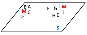
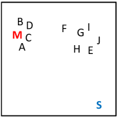
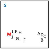
$\bm{W}_{1}$ $\swarrow$ $\searrow$ $\bm{W}_{2}$ (a) Observed view 1 (b) Observed view 2

Figure 1: A multi-view anomaly ‘M’ and a single-view anomaly ‘S’ in a two-view data set. Each letter represents an instance, and the same letter indicates the same instance. $\bm{W}_{d}$ is a projection matrix for view $d$.

Multi-view anomaly detection can be used for many applications, such as information disparity management (Duh et al, 2013), purchase behavior analysis (Gao et al, 2011), malicious insider detection (Liu and Lam, 2012), and user aggregation from multiple databases. In information disparity management, multiple views can be obtained from documents written in different languages such as Wikipedia. Multi-view anomaly detection tries to find documents that contain different information across different languages. In purchase behavior analysis, multiple views for each item can be defined as its genre and its purchase history, i.e. a set of users who purchased the item. Multi-view anomaly detection can find movies inconsistently purchased by users based on the movie genre.

We propose a probabilistic latent variable model for multi-view anomaly detection. With the proposed model, there is a latent space that is shared across all views. We assume that all views of a non-anomalous (normal) instance are generated using a single latent vector. On the other hand, an anomalous instance is assumed to have multiple latent vectors, and its different views are generated using different latent vectors, which indicates inconsistency across different views of the instance. Figure 1 (c) shows an example of a latent space shared by the two-view data. Two views of every non multi-view anomaly can be generated from a latent vector using view-dependent projection matrices. On the other hand, since two views of multi-view anomaly ‘M’ are not consistent, two latent vectors are required to generate the two views using the projection matrices.

Since the number of latent vectors for each instance is unknown, we automatically infer it from the given data by using Dirichlet process priors. The inference of the proposed model is based on a stochastic EM algorithm. In the E-step, a latent vector is assigned for each view of each instance using collapsed Gibbs sampling while analytically integrating out latent vectors. In the M-step, projection matrices for mapping latent vectors into observations are estimated by maximizing the joint likelihood. By alternately iterating E- and M-steps, we infer the number of latent vectors used in each instance and calculate its anomaly score from the probability of using more than one latent vector.

The proposed model can be seen as a robust extension of probabilistic canonical correlation analysis (PCCA) (Bach and Jordan, 2005; Wang, 2007). PCCA assumes that each instance has a latent vector, and the estimated parameters suffer effects from anomalies. In contrast, by preparing multiple latent vectors for anomalies, the proposed model can infer latent vectors and projection matrices properly without influence of multi-view anomalies.

2 Related Work

Anomaly detection has had a wide variety of applications, such as credit card fraud detection (Aleskerov et al, 1997), intrusion detection for network security (Portnoy et al, 2001), and analysis for healthcare data (Antonie et al, 2001). However, most existing anomaly detection techniques assume data with a single view, i.e. a single observation feature set.

A number of anomaly detection methods for two-view data have been proposed (Gao et al, 2010; Shekhar et al, 2002; Song et al, 2007; Sun et al, 2005; Wang and Davidson, 2009). However, they cannot be used for data with more than two views. Gao et al (2011) proposed a HOrizontal Anomaly Detection algorithm (HOAD) for finding anomalies from multi-view data. With HOAD, all views of all instances are simultaneously embedded in a low-dimensional space with the constraints that different views of the same instance are embedded close together using a spectral framework (Ng et al, 2002). Then, anomalies are detected according to distance between the embedded locations of different views of each instance. In HOAD, there are hyperparameters including a weight for the constraint that require the data to be labeled as anomalous or not for tuning, and the performance is sensitive to the hyperparameters. On the other hand, the parameters with the proposed model can be estimated from the given multi-view data without label information by maximizing the likelihood. In addition, because the proposed model is a probabilistic generative model, we can extend it in a probabilistically principled manner, for example, for handling missing data and combining with other probabilistic models. Liu and Lam (2012) proposed multi-view anomaly detection methods using consensus clustering. They found anomalies based on the inconsistency of clustering results across multiple views. Therefore, they cannot find inconsistency within a cluster. Christoudias et al (2008) proposed a method for filtering instances that are corrupted by background noise from multi-view data. The multi-view anomalies considered in this paper include not only instances corrupted by background noise but also instances categorized into different foreground classes across views, and instances with inconsistent views even if they belong to the same cluster.

The proposed model is related to probabilistic canonical correlation analysis (PCCA). When every instance has only one latent vector, the proposed model can be seen as PCCA. PCCA, or canonical correlation analysis (CCA), can be used for multi-view anomaly detection. With PCCA, a latent vector that is shared by all views for each instance and a linear projection matrix for each view are estimated by maximizing the likelihood, or minimizing the reconstruction error of the given data. The reconstruction error for each instance can be used as an anomaly score. However, the reconstruction errors are not reliable because they are calculated from parameters that are estimated using data with anomalies by assuming that all of the instances are non-anomalous. On the other hand, because the proposed model simultaneously estimates the parameters and infers anomalies, the estimated parameters are not contaminated by the anomalies. With some CCA-related methods, each latent vector is factorized into shared and private components across different views (Archambeau and Bach, 2009; Jia et al, 2010; Salzmann et al, 2010; Virtanen et al, 2011). They assume that every instance has shared and private parts that are the same dimensionality for all instances, and they cannot be used for multi-view anomaly detection. In contrast, the proposed model can detect anomalies by assuming that non-anomalous instances have only shared latent vectors, and anomalies have private latent vectors. Recently, Alvarez et al (2013) proposed a multi-view anomaly detection method. However, since the method is based on clustering, it cannot find anomalies when there are no clusters in the given data.

3 Proposed Model

Suppose that we are given $N$ instances with $D$ views $\bm{X}=\{\bm{X}_{n}\}_{n=1}^{N}$, where $\bm{X}_{n}=\{\bm{x}_{nd}\}_{d=1}^{D}$ is a set of multi-view observation vectors for the $n$th instance, and $\bm{x}_{nd}\in\mathbb{R}^{M_{d}}$ is the observation vector of the $d$th view. The task is to find anomalous instances that have inconsistent observation features across multiple views.

We propose a probabilistic latent variable model for this task. The proposed model assumes that each instance has potentially a countably infinite number of latent vectors $\bm{Z}_{n}=\{\bm{z}_{nj}\}_{j=1}^{\infty}$, where $\bm{z}_{nj}\in\mathbb{R}^{K}$. Each view of an instance $\bm{x}_{nd}$ is generated depending on a view-specific projection matrix $\bm{W}_{d}\in\mathbb{R}^{M_{d}\times K}$ and a latent vector $\bm{z}_{ns_{nd}}$that is selected from a set of latent vectors $\bm{Z}_{n}$. Here, $s_{nd}\in\{1,\cdots,\infty\}$ is the latent vector assignment of $\bm{x}_{nd}$. When the instance is non-anomalous and all its views are consistent, all of the views are generated from a single latent vector. In other words, the latent vector assignments for all views are the same, $s_{n1}=s_{n2}=\cdots=s_{nD}$. When it is an anomaly and some views are inconsistent, different views are generated from different latent vectors, and some latent vector assignments are different, i.e. $s_{nd}\neq s_{nd^{\prime}}$ for some $d\neq d^{\prime}$.

Specifically, the proposed model is an infinite mixture model, where the probability for the $d$th view of the $n$th instance is given by

$$p(\bm{x}_{nd}|\bm{Z}_{n},\bm{W}_{d},\bm{\theta}_{n},\alpha)=\sum_{j=1}^{\infty}\theta_{nj}{\cal N}(\bm{x}_{nd}|\bm{W}_{d}\bm{z}_{nj},\alpha^{-1}\bm{I}),$$ (1)

where $\bm{\theta}_{n}=\{\theta_{nj}\}_{j=1}^{\infty}$ are the mixture weights, $\theta_{nj}$ represents the probability of choosing the $j$th latent vector, $\alpha$ is a precision parameter, ${\cal N}(\bm{\mu},\bm{\Sigma})$ denotes the Gaussian distribution with mean $\bm{\mu}$ and covariance matrix $\bm{\Sigma}$, and $\bm{I}$ is the identity matrix. We use a Dirichlet process for the prior of mixture weight $\bm{\theta}_{n}$. Its use enables us to automatically infer the number of latent vectors for each instance from the given data.

The complete generative process of the proposed model for multi-view instances $\bm{X}$ is as follows,

1. Draw a precision parameter
   $\alpha\sim\text{Gamma}(a,b)$

2. For each instance: $n=1,\dots,N$

   1. Draw mixture weights
      $\bm{\theta}_{n}\sim\text{Stick}(\gamma)$

   2. For each latent vector: $j=1,\dots,\infty$

      1. Draw a latent vector
         $\bm{z}_{nj}\sim{\cal N}(\bm{0},(\alpha r)^{-1}\bm{I})$

   3. For each view: $d=1,\dots,D$

      1. Draw a latent vector assignment
         $s_{nd}\sim\text{Discrete}(\bm{\theta}_{n})$

      2. Draw an observation vector
         $\bm{x}_{nd}\sim{\cal N}(\bm{W}_{d}\bm{z}_{ns_{nd}},\alpha^{-1}\bm{I})$

Here, $\text{Stick}(\gamma)$ is the stick-breaking process (Sethuraman, 1994) that generates mixture weights for a Dirichlet process with concentration parameter $\gamma$, and $r$ is the relative precision for latent vectors. $\alpha$ is shared for observation and latent vector precision because it makes it possible to analytically integrate out $\alpha$ as shown in (4). Figure 2 shows a graphical model representation of the proposed model, where the shaded and unshaded nodes indicate observed and latent variables, respectively.

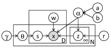
Figure 2: Graphical model representation of the proposed model.

The joint probability of the data $\bm{X}$ and the latent vector assignments $\bm{S}=\{\{s_{nd}\}_{d=1}^{D}\}_{n=1}^{N}$ is given by

$$p(\bm{X},\bm{S}|\bm{W},a,b,r,\gamma)=p(\bm{S}|\gamma)p(\bm{X}|\bm{S},\bm{W},a,b,r),$$ (2)

where $\bm{W}=\{\bm{W}_{d}\}_{d=1}^{D}$. Because we use conjugate priors, we can analytically integrate out mixture weights $\bm{\Theta}=\{\bm{\theta}_{n}\}_{n=1}^{N}$, latent vectors $\bm{Z}$, and precision parameter $\alpha$. Here, we use a Dirichlet process prior for multinomial parameter $\bm{\theta}_{n}$, and a Gaussian-Gamma prior for latent vector $\bm{z}_{nj}$. By integrating out mixture weights $\bm{\Theta}$, the first factor is calculated by

$$p(\bm{S}|\gamma)=\prod_{n=1}^{N}\frac{\gamma^{J_{n}}\prod_{j=1}^{J_{n}}(N_{nj}-1)!}{\gamma(\gamma+1)\cdots(\gamma+D-1)},$$ (3)

where $N_{nj}$ represents the number of views assigned to the $j$th latent vector in the $n$th instance, and $J_{n}$ is the number of latent vectors of the $n$th instance for which $N_{nj}>0$. By integrating out latent vectors $\bm{Z}$ and precision parameter $\alpha$, the second factor of (2) is calculated by

$$p(\bm{X}|\bm{S},\bm{W},a,b,r)=(2\pi)^{-\frac{N\sum_{d}M_{d}}{2}}r^{\frac{K\sum_{n}J_{n}}{2}}\frac{b^{a}}{b^{\prime a^{\prime}}}\frac{\Gamma(a^{\prime})}{\Gamma(a)}\prod_{n=1}^{N}\prod_{j=1}^{J_{n}}|\bm{C}_{nj}|^{\frac{1}{2}},$$ (4)

where

$$a^{\prime}=a+\frac{N\sum_{d=1}^{D}M_{d}}{2},$$ (5)

$$b^{\prime}=b+\frac{1}{2}\sum_{n=1}^{N}\sum_{d=1}^{D}\bm{x}_{nd}^{\top}\bm{x}_{nd}-\frac{1}{2}\sum_{n=1}^{N}\sum_{j=1}^{J_{n}}\bm{\mu}_{nj}^{\top}\bm{C}_{nj}^{-1}\bm{\mu}_{nj},$$ (6)

$$\bm{\mu}_{nj}=\bm{C}_{nj}\sum_{d:s_{nd}=j}\bm{W}_{d}^{\top}\bm{x}_{nd},$$ (7)

$$\bm{C}_{nj}^{-1}=\sum_{d:s_{nd}=j}\bm{W}_{d}^{\top}\bm{W}_{d}+r\bm{I}.$$ (8)

The posterior for the precision parameter $\alpha$ is given by

$$p(\alpha|\bm{X},\bm{S},\bm{W},a,b)=\text{Gamma}(a^{\prime},b^{\prime}),$$ (9)

and the posterior for the latent vector $\bm{z}_{nj}$ is given by

$$p(\bm{z}_{nj}|\bm{X},\bm{S},\bm{W},r)=\mathcal{N}(\bm{\mu}_{nj},\alpha^{-1}\bm{C}_{nj}).$$ (10)

The proposed model is a generalization of either probabilistic principal component analysis (PPCA) (Tipping and Bishop, 1999) or probabilistic canonical correlation analysis (PCCA). When all views are generated from different latent vectors for every instance, the proposed model corresponds to PPCA that is performed independently for each view. When all views are generated from a single latent vector for every instance, the proposed model corresponds to PCCA with spherical noise.

4 Inference

We describe inference procedures for the proposed model based on a stochastic EM algorithm, in which collapsed Gibbs sampling of latent vector assignments $\bm{S}$ and the maximum joint likelihood estimation of projection matrices $\bm{W}$ are alternately iterated while analytically integrating out the latent vectors $\bm{Z}$, mixture weights $\bm{\Theta}$ and precision parameter $\alpha$. By integrating out latent vectors, we do not need to explicitly infer the latent vectors, leading to a robust and fast-mixing inference.

Let $\ell=(n,d)$ be the index of the $d$th view of the $n$th instance for notational convenience. In the E-step, given the current state of all but one latent assignment $s_{\ell}$, a new value for $s_{\ell}$ is sampled from $\{1,\cdots,J_{n\setminus\ell}+1\}$ according to the following probability,

$$p(s_{\ell}=j|\bm{X},\bm{S}_{\setminus\ell},\bm{W},a,b,r,\gamma)\propto\frac{p(s_{\ell}=j,\bm{S}_{\setminus\ell}|\gamma)}{p(\bm{S}_{\setminus\ell}|\gamma)}\cdot\frac{p(\bm{X}|s_{\ell}=j,\bm{S}_{\setminus\ell},\bm{W},a,b,r)}{p(\bm{X}_{\setminus\ell}|\bm{S}_{\setminus\ell},\bm{W},a,b,r)},$$ (11)

where $\setminus\ell$ represents a value or set excluding the $d$th view of the $n$th instance.

The first factor is given by

$$\frac{p(s_{\ell}=j,\bm{S}_{\setminus\ell}|\gamma)}{p(\bm{S}_{\setminus\ell}|\gamma)}=\left\{\begin{array}[]{ll}\frac{N_{nj\setminus\ell}}{D-1+\gamma}&\text{if $j\leq J_{n\setminus\ell}$}\\ \frac{\gamma}{D-1+\gamma}&\text{if $j=J_{n\setminus\ell}+1$},\\ \end{array}\right.$$ (14)

using (3), where $j\leq J_{n\setminus\ell}$ is for existing latent vectors, and $j=J_{n\setminus\ell}+1$ is for a new latent vector. By using (4), the second factor is given by

$$\frac{p(\bm{X}|s_{\ell}=j,\bm{S}_{\setminus\ell},\bm{W},a,b,r)}{p(\bm{X}_{\setminus\ell}|\bm{S}_{\setminus\ell},\bm{W},a,b,r)}$$

$$=(2\pi)^{-\frac{M_{d}}{2}}r^{I(j=J_{n\setminus\ell}+1)\frac{K}{2}}\frac{b_{\setminus\ell}^{\prime a_{\setminus\ell}^{\prime}}}{b_{s_{\ell}=j}^{\prime a_{s_{\ell}=j}^{\prime}}}\frac{\Gamma(a_{s_{\ell}=j}^{\prime})}{\Gamma(a_{\setminus\ell}^{\prime})}\frac{|\bm{C}_{j,s_{\ell}=j}|^{\frac{1}{2}}}{|\bm{C}_{j\setminus\ell}|^{\frac{1}{2}}},$$ (15)

where $I(\cdot)$ represents the indicator function, i.e. $I(A)=1$ if $A$ is true and $0$ otherwise, and subscript $s_{\ell}=j$ indicates the value when $\bm{x}_{\ell}$ is assigned to the $j$th latent vector as follows,

$$a_{s_{\ell}=j}^{\prime}=a^{\prime},$$ (16)

$$b_{s_{\ell}=j}^{\prime}=b_{\setminus\ell}^{\prime}+\frac{1}{2}\bm{x}_{\ell}^{\top}\bm{x}_{\ell}+\frac{1}{2}\bm{\mu}_{nj\setminus\ell}^{\top}\bm{C}_{nj\setminus\ell}^{-1}\bm{\mu}_{nj\setminus\ell}-\frac{1}{2}\bm{\mu}_{nj,s_{\ell}=j}^{\top}\bm{C}_{nj,s_{\ell}=j}^{-1}\bm{\mu}_{nj,s_{\ell}=j},$$ (17)

$$\bm{\mu}_{nj,s_{\ell}=j}=\bm{C}_{nj,s_{\ell}=j}(\bm{W}_{d}^{\top}\bm{x}_{\ell}+\bm{C}_{nj\setminus\ell}^{-1}\bm{\mu}_{nj\setminus\ell}),$$ (18)

$$\bm{C}_{nj,s_{\ell}=j}^{-1}=\bm{W}_{d}^{\top}\bm{W}_{d}+\bm{C}_{nj\setminus\ell}^{-1}.$$ (19)

Intuitively, if the current view cannot be modeled well by existing latent vectors, a new latent vector is used, which indicates that the view is inconsistent with the other views.

In the M-step, the projection matrices $\bm{W}$ are estimated by maximizing the logarithm of the joint likelihood (2). We can maximize the likelihood by using a gradient-based numerical optimization method such as the quasi-Newton method (Nocedal, 1980). The gradient of the joint log likelihood is calculated by

$$\frac{\partial\log p(\bm{X},\bm{S}|\bm{W},a,b,r,\gamma)}{\partial\bm{W}_{d}}$$

$$=-\bm{W}_{d}\sum_{n=1}^{N}\sum_{j=1}^{J_{n}}\bm{C}_{nj}-\frac{a^{\prime}}{b^{\prime}}\sum_{n=1}^{N}\Bigl{(}\bm{W}_{d}\bm{\mu}_{ns_{nd}}\bm{\mu}_{ns_{nd}}^{\top}-\bm{x}_{nd}\bm{\mu}_{ns_{nd}}^{\top}\Bigr{)}.$$ (20)

When we iterate the E-step that samples the latent vector assignment $s_{nd}$ by employing (11) for each view $d=1,\dots,D$ in each instance $n=1,\dots,N$, and the M-step that maximizes the joint likelihood using (20) with respect to the projection matrix $\bm{W}_{d}$ for each view $d=1,\dots,D$, we obtain an estimate of the latent vector assignments and projection matrices.

For an anomaly score, we use the probability that the instance uses more than one latent vector. It is estimated by using the samples obtained in the inference as follows,

$$v_{n}=\frac{1}{H}\sum_{h=1}^{H}I(J_{n}^{(h)}>1),$$ (21)

where $J_{n}^{(h)}$ is the number of latent vectors used by the $n$th instance in the $h$th iteration of the Gibbs sampling after the burn-in period, and $H$ is the number of the iterations.

We can use cross-validation to select an appropriate dimensionality for the latent space $K$. With cross-validation, we assume that some features are missing from the given data, and infer the model with a different $K$. Then, we select the smallest $K$ value that has performed the best at predicting missing values.

5 Experiments

5.1 Data

We evaluated the proposed model quantitatively by using 11 data sets, which we obtained from the LIBSVM data sets (Chang and Lin, 2011). We generated multiple views by randomly splitting the features, and anomalies were added by swapping views of two randomly selected instances as Gao et al (2011) did in their experiments. Splitting data does not generate anomalies. Therefore, we can evaluate methods while controlling the anomaly rate properly. By swapping, although single-view anomalies cannot be created since the distribution for each view does not change, multi-view anomalies are created.

5.2 Comparing methods

We compared the proposed model with probabilistic canonical correlation analysis (PCCA), horizontal anomaly detection (HOAD) (Gao et al, 2011), consensus clustering based anomaly detection (CC) (Liu and Lam, 2012), and one-class support vector machine (OCSVM) (Schölkopf et al, 2001). For PCCA, we used the proposed model in which the number of latent vectors was fixed at one for every instance. The anomaly scores obtained with PCCA were calculated based on the reconstruction errors. HOAD requires to select an appropriate hyperparameter value for controlling the constraints whereby different views of the same instance are embedded close together. We ran HOAD with different hyperparameter settings $\{0.1,1,10,100\}$, and show the results that achieved the highest performance for each data set. For CC, first we clustered instances for each view using spectral clustering (Ng et al, 2002). We set the number of clusters at 20, which achieved a good performance in preliminary experiments. Then, we calculated anomaly scores by the likelihood of consensus clustering when an instance was removed. OCSVM is a representative method for single-view anomaly detection. To investigate the performance of a single-view method for multi-view anomaly detection, we included OCSVM as a comparison method. For OCSVM, multiple views are concatenated in a single vector, then use it for the input. We used Gaussian kernel. In the proposed model, we used $\gamma=1$, $a=1$, and $b=1$ for all experiments. The number of iterations for the Gibbs sampling was 500, and the anomaly score was calculated by averaging over the multiple samples.

5.3 Multi-view anomaly detection

For the evaluation measurement, we used the area under the ROC curve (AUC). A higher AUC indicates a higher anomaly detection performance. Figure 3 shows AUCs with different rates of anomalies using two-view data sets, which are averaged over 50 experiments. For the dimensionality of the latent space, we used $K=5$ for the proposed model, PCCA, and HOAD. In general, as the anomaly rate increases, the performance decreases. The proposed model achieved the best performance with eight of the 11 data sets. This result indicates that the proposed model can find anomalies effectively by inferring a number of latent vectors for each instance. The performance of CC was low because it assumes that there are clusters for each view, and it cannot find anomalies within clusters. The AUC of OCSVM was low, because it is a single-view anomaly detection method, which considers instances anomalous that are different from others within a single view. Multi-view anomaly detection is the task to find instances that have inconsistent features across views, but not inconsistent features within a view. The computational time needed for PCCA was 2 sec, and that needed for the proposed model was 35 sec with wine data.

Figure 4 shows AUCs with different numbers of views. For many cases with different latent dimensionalities and different numbers of views, the proposed model achieved the best performance.

Figure 5 shows AUCs with different dimensionalities of latent vectors using data sets whose anomaly rate is 0.4. When the dimensionality was very low ($K=1$ or $2$), the AUC was low in most of the data sets, because low-dimensional latent vectors cannot represent the observation vectors well. With all the methods, the AUCs were relatively stable when the latent dimensionality was higher than four.

(a) breast-cancer	(b) diabetes
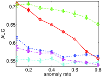
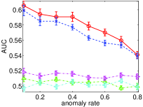
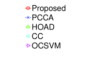
(c) glass	(d) heart	(e) ionosphere
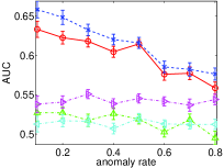
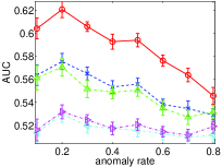
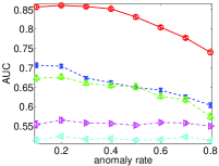
(f) sonar	(g) svmguide2	(h) svmguide4
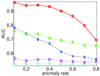
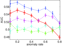
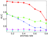
(i) vehicle	(j) vowel	(k) wine

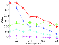
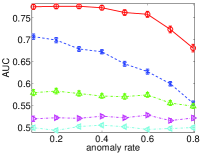
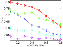
Figure 3: Average AUCs with different anomaly rates, and their standard errors. A higher AUC is better.

(a) breast-cancer	(b) diabetes
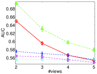
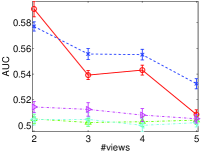
(c) glass	(d) heart	(e) ionosphere
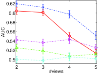
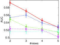
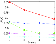
(f) sonar	(g) svmguide2	(h) svmguide4
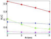
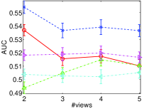
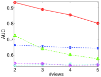
(i) vehicle	(j) vowel	(k) wine

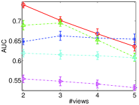
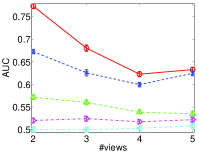
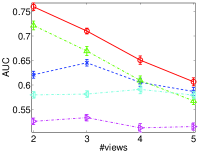
Figure 4: Average AUCs with different numbers of views, and their standard errors.

(a) breast-cancer	(b) diabetes
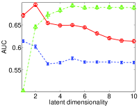
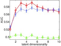
(c) glass	(d) heart	(e) ionosphere
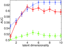
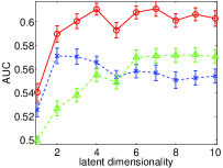
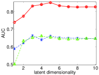
(f) sonar	(g) svmguide2	(h) svmguide4
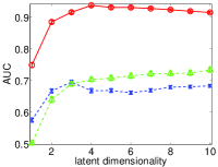
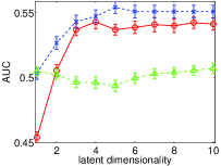
(i) vehicle	(j) vowel	(k) wine

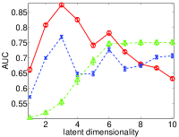
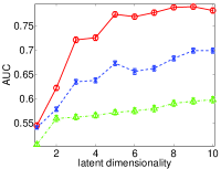
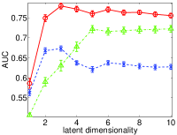
Figure 5: Average AUCs with different dimensionalities of latent vectors, and ther standard errors.

5.4 Single-view anomaly detection

We illustrated that the proposed model does not detect single-view anomalies using synthetic single-view anomaly data. With the synthetic data, latent vectors for single-view anomalies were generated from ${\cal N}(\bm{0},\sqrt{10}\bm{I})$, and those for non-anomalous instances were generated from ${\cal N}(\bm{0},\bm{I})$. Since each of the anomalies has only one single latent vector, it is not a multi-view anomaly. The numbers of anomalous and non-anomalous instances were 5 and 95, respectively. The dimensionalities of the observed and latent spaces were five and three, respectively. Table 1 shows the average AUCs with the single-view anomaly data, which are averaged over 50 different data sets. The low AUC of the proposed model indicates that it does not consider single-view anomalies as anomalies. On the other hand, the AUC of the one-class SVM (OCSVM) was high because OCSVM is a single-view anomaly detection method, and it leads to low multi-view anomaly detection performance.

Table 1: Average AUCs for single-view anomaly detection.

Proposed	PCCA	OCSVM
$\mathbf{0.117}\pm 0.098$	$0.174\pm 0.095$	$0.860\pm 0.232$

5.5 Missing value imputation

We can use the proposed model for missing value imputation in multi-view data with anomalies. The proposed model was evaluated by comparison with PCCA and Average, which estimates missing values by averaging the observation features over instances. We randomly selected 5% of the values as missing. Table 2 shows the mean squared errors for missing value imputation with data sets whose anomaly rate is 0.4. For all of the data sets, the proposed model achieved the lowest error. This result shows the effectiveness of the proposed model for imputing missing values in multi-view data with anomalies.

Table 2: Average mean squared errors for imputing missing values. Values in bold typeface are statistically better at the $5\%$ level from those in normal typeface as indicated by a paired t-test.

	breast-cancer	diabetes	glass	heart	ionosphere	sonar
Proposed	$\mathbf{0.532}$	$\mathbf{0.052}$	$\mathbf{0.073}$	$\mathbf{0.797}$	$\mathbf{0.771}$	$\mathbf{1.510}$
PCCA	$0.574$	$0.063$	$0.096$	$1.146$	$0.935$	$1.800$
Average	$2.190$	$0.313$	$1.045$	$3.305$	$2.708$	$3.754$
	svmguide2	svmguide4	vehicle	vowel	wine
Proposed	$\mathbf{0.003}$	$\mathbf{1.497}$	$\mathbf{0.118}$	$\mathbf{0.150}$	$\mathbf{0.201}$
PCCA	$\mathbf{0.003}$	$1.680$	$\mathbf{0.177}$	$0.208$	$0.255$
Average	$0.004$	$3.717$	$1.767$	$0.521$	$1.419$

5.6 Latent dimensionality estimation

We also evaluated the performance of the proposed model to estimate the latent dimensionality from the given data. For this purpose, we used synthetic data sets, where the true latent dimensionality was known. Synthetic data sets with two views were generated according to the following procedure. First, we sampled a latent vector for each non-anomalous instance, and two latent vectors for each anomaly from a $K^{\star}$-dimensional Gaussian distribution with mean $\bm{0}$ and covariance $\bm{I}$. Here, $K^{\star}$ is the true latent dimensionality, and we used $K^{\star}=5$. Second, we generated projection matrices $\bm{W}$ where each element was drawn from a Gaussian distribution with mean $0$ and variance 1. Finally, we generated observations using the latent vectors and projection matrices with Gaussian noise. Figure 6 shows the mean squared errors for missing value imputation using synthetic data sets with different anomaly rates when the latent dimensionality of the proposed model was changed, $K\in\{2,\cdots,10\}$. With the proposed model, the mean squared errors decreased rapidly when $K<5$, and they did not vary greatly when $K\geq 5$, in all of the data sets with different anomaly rates. This result indicates that the proposed model can estimate the latent dimensionality from multi-view data with anomalies. In contrast, with PCCA, the mean squared errors decreased even when $K>5$ especially in data sets with high anomaly rates. This implies that PCCA requires a higher latent dimensionality for modeling data with anomalies than the true latent dimensionality. When the anomaly rate is small, the proposed model and PCCA perform similarly as shown in Figure 6 (a). Because we use Bayesian inference for the proposed model and PCCA based on Markov chain Monte Carlo in our experiments, we can avoid overfitting when the latent dimensionality is higher than the true dimensionality as shown in Bayesian probabilistic matrix factorization (Salakhutdinov and Mnih, 2008).

(a) anomaly rate: 0.2	(b) anomaly rate: 0.4
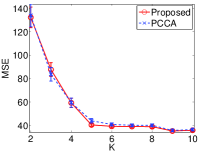
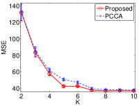
(c) anomaly rate: 0.6	(d) anomaly rate: 0.8

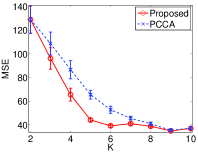
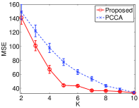
Figure 6: Average mean squared errors for imputing missing values and their standard errors with different latent dimensionalities using synthetic data sets with different anomaly rates.

5.7 Application to movie data

For an application of multi-view anomaly detection, we analyzed inconsistency between movie rating behavior and genre in MovieLens data (Herlocker et al, 1999). An instance corresponds to a movie, where the first view represents whether the movie is rated or not by users, and the second view represents the movie genre. Both views consists of binary features. We used 338 movies, 943 users and 19 genres. Table 3 shows high and low anomaly score movies when we analyzed the movie data by the proposed method with $K=5$. ‘The Full Monty’ and ‘Liar Liar’ were categorized in ‘Comedy’ genre. They are rated by not only users who likes ‘Comedy’, but also who likes ‘Romance’ and ‘Action-Thriller’. ‘The Professional’ was anomaly because it was rated by two different user groups, where a group prefers ‘Romance’ and the other prefers ‘Action’. Since ‘Star Trek’ series are typical Sci-Fi and liked by specific users, its anomaly score was low.

Table 3: High and low anomaly score movies calculated by the proposed model.

Title	Score	Title	Score
The Full Monty	0.98	Star Trek VI	0.04
Liar Liar	0.93	Star Trek III	0.04
The Professional	0.91	The Saint	0.04
Mr. Holland’s Opus	0.88	Heat	0.03
Contact	0.87	Conspiracy Theory	0.03

6 Conclusion

We proposed a generative model approach for multi-view anomaly detection, which finds instances that have inconsistent views. In the experiments, we confirmed that the proposed model could perform much better than existing methods for detecting multi-view anomalies, and for imputing missing values in multi-view data with anomalies. There are several avenues that can be pursued for future work. The proposed model assumes the linearity of observations with respect to their latent vectors. We can relax this assumption by using Gaussian processes (Lawrence, 2004; Rasmussen and Williams, 2005; Shon et al, 2006). We would like to evaluate our proposed model for other real applications. CCA is successfully used for a wide variety of real multi-view data, such as multilingual data and image-annotation data. This indicates that the proposed model based on CCA can handle the same wide variety of real data.

References

- Aleskerov et al (1997) Aleskerov E, Freisleben B, Rao B (1997) Cardwatch: A neural network based database mining system for credit card fraud detection. In: Computational intelligence for financial engineering. Proceedings of the IEEE/IAFE, pp 220–226
- Alvarez et al (2013) Alvarez AM, Yamada M, Kimura A, Iwata T (2013) Clustering-based anomaly detection in multi-view data. In: Proceedings of ACM International Conference on Information and Knowledge Management, CIKM
- Antonie et al (2001) Antonie ML, Zaiane OR, Coman A (2001) Application of data mining techniques for medical image classification. MDM/KDD pp 94–101
- Archambeau and Bach (2009) Archambeau C, Bach FR (2009) Sparse probabilistic projections. In: Neural Information Processing Systems, MIT Press, NIPS, pp 17–24
- Bach and Jordan (2005) Bach FR, Jordan MI (2005) A probabilistic interpretation of canonical correlation analysis. Tech. Rep. 688, Department of Statistics, University of California, Berkeley
- Bickel and Scheffer (2004) Bickel S, Scheffer T (2004) Multi-view clustering. In: ICDM, vol 4, pp 19–26
- Blum and Mitchell (1998) Blum A, Mitchell T (1998) Combining labeled and unlabeled data with co-training. In: Proceedings of the eleventh annual conference on Computational learning theory, ACM, pp 92–100
- Chandola et al (2009) Chandola V, Banerjee A, Kumar V (2009) Anomaly detection: A survey. ACM Computing Surveys (CSUR) 41(3):15
- Chang and Lin (2011) Chang C, Lin C (2011) LIBSVM: a library for support vector machines. ACM Transactions on Intelligent Systems and Technology (TIST) 2(3):27
- Christoudias et al (2008) Christoudias CM, Urtasun R, Darrell T (2008) Multi-view learning in the presence of view disagreement. In: Proceedings of the 24th Conference on Unvertainty in Artificial Intelligence, UAI
- Duh et al (2013) Duh K, Yeung CMA, Iwata T, Nagata M (2013) Managing information disparity in multilingual document collections. ACM Transactions on Speech and Language Processing (TSLP) 10(1):1
- Gao et al (2010) Gao J, Liang F, Fan W, Wang C, Sun Y, Han J (2010) On community outliers and their efficient detection in information networks. In: Proceedings of the 16th ACM SIGKDD International Conference on Knowledge Discovery and Data Mining, ACM, pp 813–822
- Gao et al (2011) Gao J, Fan W, Turaga D, Parthasarathy S, Han J (2011) A spectral framework for detecting inconsistency across multi-source object relationships. In: IEEE 11th International Conference on Data Mining (ICDM), IEEE, pp 1050–1055
- Herlocker et al (1999) Herlocker JL, Konstan JA, Borchers A, Riedl J (1999) An algorithmic framework for performing collaborative filtering. In: Proceedings of the 22nd annual international ACM SIGIR conference on Research and development in information retrieval, ACM, pp 230–237
- Jia et al (2010) Jia Y, Salzmann M, Darrell T (2010) Factorized latent spaces with structured sparsity. Advances in Neural Information Processing Systems 23:982–990
- Lawrence (2004) Lawrence ND (2004) Gaussian process latent variable models for visualisation of high dimensional data. Advances in Neural Information Processing Systems 16(3):329–336
- Liu and Lam (2012) Liu AY, Lam DN (2012) Using consensus clustering for multi-view anomaly detection. In: 2012 IEEE Symposium on Security and Privacy Workshops (SPW), IEEE, pp 117–124
- Ng et al (2002) Ng AY, Jordan MI, Weiss Y, et al (2002) On spectral clustering: Analysis and an algorithm. In: Advances in Neural Information Processing Systems, pp 849–856
- Nocedal (1980) Nocedal J (1980) Updating quasi-Newton matrices with limited storage. Mathematics of computation 35(151):773–782
- Portnoy et al (2001) Portnoy L, Eskin E, Stolfo S (2001) Intrusion detection with unlabeled data using clustering. In: Proceedings of ACM CSS Workshop on Data Mining Applied to Security
- Rasmussen and Williams (2005) Rasmussen CE, Williams CK (2005) Gaussian Processes for Machine Learning. The MIT Press
- Salakhutdinov and Mnih (2008) Salakhutdinov R, Mnih A (2008) Bayesian probabilistic matrix factorization using Markov chain Monte Carlo. In: Proceedings of the 25th International Conference on Machine Learning, ICML ’08, pp 880–887
- Salzmann et al (2010) Salzmann M, Ek CH, Urtasun R, Darrell T (2010) Factorized orthogonal latent spaces. In: International Conference on Artificial Intelligence and Statistics, pp 701–708
- Schölkopf et al (2001) Schölkopf B, Platt JC, Shawe-Taylor J, Smola AJ, Williamson RC (2001) Estimating the support of a high-dimensional distribution. Neural computation 13(7):1443–1471
- Sethuraman (1994) Sethuraman J (1994) A constructive definition of Dirichlet priors. Statistica Sinica 4:639–650
- Shekhar et al (2002) Shekhar S, Lu CT, Zhang P (2002) Detecting graph-based spatial outliers. Intelligent Data Analysis 6(5):451–468
- Shon et al (2006) Shon A, Grochow K, Hertzmann A, Rao R (2006) Learning shared latent structure for image synthesis and robotic imitation. Advances in Neural Information Processing Systems 18:1233–1240
- Sindhwani and Rosenberg (2008) Sindhwani V, Rosenberg DS (2008) An RKHS for multi-view learning and manifold co-regularization. In: Proceedings of the 25th International Conference on Machine learning, ACM, pp 976–983
- Song et al (2007) Song X, Wu M, Jermaine C, Ranka S (2007) Conditional anomaly detection. IEEE Transactions on Knowledge and Data Engineering 19(5):631–645
- Sun et al (2005) Sun J, Qu H, Chakrabarti D, Faloutsos C (2005) Neighborhood formation and anomaly detection in bipartite graphs. In: Proceedings of the 5th IEEE International Conference on Data Mining, IEEE, pp 418–425
- Tipping and Bishop (1999) Tipping M, Bishop C (1999) Probabilistic principal component analysis. Journal of the Royal Statistical Society: Series B (Statistical Methodology) 61(3):611–622
- Virtanen et al (2011) Virtanen S, Klami A, Kaski S (2011) Bayesian CCA via group sparsity. In: Proceedings of the 28th International Conference on Machine Learning, ICML ’11, pp 457–464
- Wang (2007) Wang C (2007) Variational Bayesian approach to canonical correlation analysis. IEEE Transactions on Neural Networks 18(3):905–910
- Wang and Davidson (2009) Wang X, Davidson I (2009) Discovering contexts and contextual outliers using random walks in graphs. In: Proceedings of the 9th IEEE International Conference on Data Mining, IEEE, pp 1034–1039