A Randomized Algorithm for CCA

Abstract

We present RandomizedCCA, a randomized algorithm for computing canonical analysis, suitable for large datasets stored either out of core or on a distributed file system. Accurate results can be obtained in as few as two data passes, which is relevant for distributed processing frameworks in which iteration is expensive (e.g., Hadoop). The strategy also provides an excellent initializer for standard iterative solutions.

1 Introduction

Canonical Correlation Analysis (CCA) is a fundamental statistical technique for characterizing the linear relationships between two multidimensional variables. First introduced in 1936 by Hotelling[10], it has found numerous applications. For the machine learning community, more familiar applications include learning with privileged information[15], semi-supervised learning[3, 14], monolingual[5] and multilingual[7] word representation learning, locality sensitive hashing[8] and clustering[2]. Because these applications involve unlabeled or partially labeled data, the amount of data available for analysis can be vast, motivating the need for scalable approaches.

2 Background

Given two view data, CCA finds a projection of each view into a common latent space which maximizes the cross-correlation, subject to each view projection having unit variance, and subject to each projection dimension being uncorrelated with other projection dimensions. In matrix form, given two views ${\mathbf{A}}\in\mathbb{R}^{n\times d_{a}}$ and ${\mathbf{B}}\in\mathbb{R}^{n\times d_{b}}$, the CCA projections ${\mathbf{X}}_{a}\in\mathbb{R}^{d_{a}\times k}$ and ${\mathbf{X}}_{b}\in\mathbb{R}^{d_{b}\times k}$ are the solution to

$$\operatorname*{maximize\;}_{{\mathbf{X}}_{a},{\mathbf{X}}_{b}} \mathrm{Tr}\left({\mathbf{X}}_{a}^{\top}{\mathbf{A}}^{\top}{\mathbf{B}}{\mathbf{X}}_{b}\right),$$

$$\operatorname*{subject\ to\;} {\mathbf{X}}_{a}^{\top}{\mathbf{A}}^{\top}{\mathbf{A}}{\mathbf{X}}_{a}=n{\mathbf{I}},$$ (1)

$${\mathbf{X}}_{b}^{\top}{\mathbf{B}}^{\top}{\mathbf{B}}{\mathbf{X}}_{b}=n{\mathbf{I}}.$$ (2)

The KKT conditions, expressed in terms of the QR-decompositions ${\mathbf{Q}}_{a}{\mathbf{R}}_{a}={\mathbf{A}}$ and ${\mathbf{Q}}_{b}{\mathbf{R}}_{b}={\mathbf{B}}$, lead to the following multivariate eigenvalue problem[4]

$$\left(\begin{array}[]{cc}0&{\mathbf{Q}}_{a}^{\top}{\mathbf{Q}}_{b}\\ {\mathbf{Q}}_{b}^{\top}{\mathbf{Q}}_{a}&0\end{array}\right)\left(\begin{array}[]{c}{\mathbf{V}}_{a}\\ {\mathbf{V}}_{b}\end{array}\right)=\left(\begin{array}[]{c}{\mathbf{V}}_{a}\\ {\mathbf{V}}_{b}\end{array}\right){\mathbf{\Lambda}},$$ (3)

subject to ${\mathbf{V}}_{a}^{\top}{\mathbf{V}}_{a}={\mathbf{I}}$, ${\mathbf{V}}_{b}^{\top}{\mathbf{V}}_{b}={\mathbf{I}}$, ${\mathbf{V}}_{a}{\mathbf{R}}_{a}={\mathbf{X}}_{a}$, and ${\mathbf{V}}_{b}{\mathbf{R}}_{b}={\mathbf{X}}_{b}$.

Equation (3) leads to several solution strategies. For moderate sized design matrices, an SVD of ${\mathbf{Q}}_{a}^{\top}{\mathbf{Q}}_{b}$ directly reveals the solution in the ${\mathbf{V}}_{a,b}$ coordinate system [1]. The transformation from ${\mathbf{V}}_{a,b}$ to ${\mathbf{X}}_{a,b}$ can be obtained from either the SVD or QR-decompositions of ${\mathbf{A}}$ and ${\mathbf{B}}$.

For larger design matrices lacking special structure, SVD and QR-decompositions are prohibitively expensive, necessitating other techniques. Large scale solutions are possible via Horst iteration [4], the analog of orthogonal power iteration for the multivariate eigenvalue problem, in which each block of variables is individually normalized following matrix multiplication [17]. For CCA, the matrix multiplication step of Horst iteration can be done directly in the ${\mathbf{X}}_{a,b}$ coordinate system via solving a least-squares problem. Furthermore, the least squares solutions need only be done approximately to ensure convergence [13]. Unfortunately, Horst iteration still requires many passes over the data for good results.

3 Algorithm

Algorithm 1 Randomized CCA

1:

2:function RandomizedCCA($k,p,q,\lambda_{a},\lambda_{b},{\mathbf{A}}\in\mathbb{R}^{n\times d_{a}},{\mathbf{B}}\in\mathbb{R}^{n\times d_{b}}$)

3:     // Randomized range finder for ${\mathbf{A}}^{\top}{\mathbf{B}}$

4:     ${\mathbf{Q}}_{a}\leftarrow\operatorname{randn}(d_{a},k+p)$ $\triangleright$ Gaussian suitable for sparse ${\mathbf{A}}$, ${\mathbf{B}}$

5:     ${\mathbf{Q}}_{b}\leftarrow\operatorname{randn}(d_{b},k+p)$ $\triangleright$ Structured randomness suitable for dense ${\mathbf{A}}$, ${\mathbf{B}}$

6:     for $i\in\{1,\ldots,q\}$ do

7:         data pass

8:              ${\mathbf{Y}}_{a}\leftarrow{\mathbf{A}}^{\top}{\mathbf{B}}{\mathbf{Q}}_{b}$

9:              ${\mathbf{Y}}_{b}\leftarrow{\mathbf{B}}^{\top}{\mathbf{A}}{\mathbf{Q}}_{a}$

10:         end data pass

11:         ${\mathbf{Q}}_{a}\leftarrow\operatorname{orth}({\mathbf{Y}}_{a})$

12:         ${\mathbf{Q}}_{b}\leftarrow\operatorname{orth}({\mathbf{Y}}_{b})$

13:     end for

14:     // Final optimization over bases ${\mathbf{Q}}_{a},{\mathbf{Q}}_{b}$

15:     data pass

16:         ${\mathbf{C}}_{a}\leftarrow{\mathbf{Q}}_{a}^{\top}{\mathbf{A}}^{\top}{\mathbf{A}}{\mathbf{Q}}_{a}$ $\triangleright$ ${\mathbf{C}}_{a}\in\mathbb{R}^{(k+p)\times(k+p)}$ is “small”

17:         ${\mathbf{C}}_{b}\leftarrow{\mathbf{Q}}_{b}^{\top}{\mathbf{B}}^{\top}{\mathbf{B}}{\mathbf{Q}}_{b}$ $\triangleright$ Similarly for ${\mathbf{C}}_{b}$, ${\mathbf{F}}$

18:         ${\mathbf{F}}\leftarrow{\mathbf{Q}}_{a}^{\top}{\mathbf{A}}^{\top}{\mathbf{B}}{\mathbf{Q}}_{b}$

19:     end data pass

20:     ${\mathbf{L}}_{a}\leftarrow\operatorname{chol}({\mathbf{C}}_{a}+\lambda_{a}{\mathbf{Q}}_{a}^{\top}{\mathbf{Q}}_{a})$ $\triangleright$ ${\mathbf{Q}}_{a}{\mathbf{L}}_{a}^{-1}=({\mathbf{A}}^{\top}{\mathbf{A}}+\lambda_{a}{\mathbf{I}})^{-1/2}{\mathbf{Q}}_{a}$

21:     ${\mathbf{L}}_{b}\leftarrow\operatorname{chol}({\mathbf{C}}_{b}+\lambda_{b}{\mathbf{Q}}_{b}^{\top}{\mathbf{Q}}_{b})$ $\triangleright$ ${\mathbf{Q}}_{b}{\mathbf{L}}_{b}^{-1}=({\mathbf{B}}^{\top}{\mathbf{B}}+\lambda_{b}{\mathbf{I}})^{-1/2}{\mathbf{Q}}_{b}$

22:     ${\mathbf{F}}\leftarrow{\mathbf{L}}_{a}^{-\top}{\mathbf{F}}{\mathbf{L}}_{b}^{-1}$

23:     $({\mathbf{U}},\Sigma,{\mathbf{V}})\leftarrow\operatorname{svd}({\mathbf{F}},k)$

24:     ${\mathbf{X}}_{a}\leftarrow\sqrt{n}{\mathbf{Q}}_{a}{\mathbf{L}}_{a}^{-1}{\mathbf{U}}$

25:     ${\mathbf{X}}_{b}\leftarrow\sqrt{n}{\mathbf{Q}}_{b}{\mathbf{L}}_{b}^{-1}{\mathbf{V}}$

26:     return $({\mathbf{X}}_{a},{\mathbf{X}}_{b},\Sigma)$

27:end function

Our proposal is RandomizedCCA outlined in Algorithm 1. For ease of exposition, we elide mean shifting of each design matrix, which is a rank one update, and can be done in $O(d_{a}+d_{b})$ extra space without introducing additional data passes and preserving sparsity. Line numbers 3 through 13 constitute a standard randomized range finder [9] with power iteration for the left and right singular spaces of ${\mathbf{A}}^{\top}{\mathbf{B}}$. If we consider ${\mathbf{Q}}_{a}$ and ${\mathbf{Q}}_{b}$ as providing a $\tilde{k}$ rank approximation to the top range of ${\mathbf{A}}^{\top}{\mathbf{B}}$, then analysis of randomized range finding indicates $\mathbb{E}\left\|{\mathbf{A}}^{\top}{\mathbf{B}}-{\mathbf{Q}}_{a}{\mathbf{Q}}_{a}^{\top}{\mathbf{A}}^{\top}{\mathbf{B}}\right\|\leq\left[1+4\frac{\sqrt{k+p}}{p-\tilde{k}-1}\sqrt{n}\right]^{1/q}\sigma_{\tilde{k}},$ and analogously for ${\mathbf{Q}}_{b}$[9]. Intuition about the relevant value of $\tilde{k}$ can be determined by considering the effect of regularization. To prevent overfitting, equations (1) and (2) are regularized with $\lambda_{a}{\mathbf{I}}$ and $\lambda_{b}{\mathbf{I}}$ respectively, hence the canonical correlations possible in the space orthogonal to the top $\tilde{k}$ range of ${\mathbf{A}}^{\top}{\mathbf{B}}$ are at most $\sigma_{\tilde{k}}/\sqrt{\lambda_{a}\lambda_{b}}$. When this quantity is below the $k^{\mathrm{th}}$ canonical correlation, the top $\tilde{k}$ range of ${\mathbf{A}}^{\top}{\mathbf{B}}$ is the only relevant subspace and the question then becomes the extent to which the randomized range finder is approximating this space well.

In practice $\tilde{k}$ is unknown and thus relative to $k$, RandomizedCCA effectively requires large amounts of oversampling (e.g., $p=1000$) to achieve good results. Nonetheless, when iterations over the data are expensive, this level of oversampling can be more computationally attractive than alternative approaches. This is because typically CCA is used to find a low dimensional embedding (e.g., $k=50$), whereas the final exact SVD and Cholesky factorizations in lines 20 through 23 can be done using a single commodity machine as long as $k+p\lesssim 10000$. Therefore there is computational headroom available for large oversampling. Ultimately the binding constraint is the utility of storing ${\mathbf{Q}}_{a,b}$ and ${\mathbf{Y}}_{a,b}$ in main memory.

4 Experimental Results

Europarl is a collection of simultaneous translated documents extracted from the proceedings of the European parliament [11]. Multilingual alignment is available at the individual sentence level. We used a single random 9:1 split of sentences into train and test sets for all experiments. We processed each sentence into a fixed dimensional representation using a bag of words representation composed with inner-product preserving hashing [16]. For these experiments we used $2^{19}$ hash slots. We used English for the ${\mathbf{A}}$ design matrix and Greek for the ${\mathbf{B}}$ design matrix, resulting in $n=1,235,976$ and $d_{a}=d_{b}=2^{19}$. Note the ultimate embedding produced by this procedure is the composition of the hashing strategy with the projections found by RandomizedCCA.

Figure 1: Spectrum of $(1/n){\mathbf{A}}^{\top}{\mathbf{B}}$.

figure The top-2000 spectrum of $(1/n){\mathbf{A}}^{\top}{\mathbf{B}}$, as estimated by two-pass randomized SVD, is shown in figure 1. This provides some intuition as to why the top range of ${\mathbf{A}}^{\top}{\mathbf{B}}$ should generate an excellent approximation to the optimal CCA solution, as the spectrum exhibits power-law decay and ultimately decreases to a point which is comparable to a plausible regularization parameter setting.

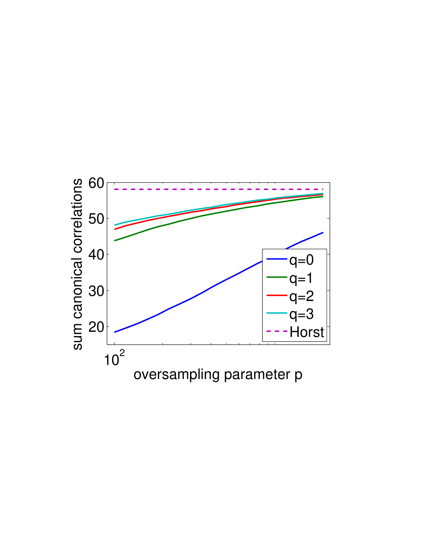
(a) $\frac{1}{n}\mathrm{Tr}\left({\mathbf{X}}_{a}{\mathbf{A}}^{\top}{\mathbf{B}}{\mathbf{X}}_{b}\right)$ for RandomizedCCA as $q$ and $p$ are varied, with $k=60$. The dashed line is the result of running Horst iteration for 120 passes over the data.

q	p	Train	Test	time (s)
0	910	38.942	38.797	190
0	2000	46.095	45.891	463
1	910	53.934	53.835	334
1	2000	56.054	55.656	770
2	910	55.017	54.782	484
2	2000	56.666	56.528	1186
3	910	55.386	54.991	637
3	2000	56.833	56.860	1412
Horst (same $\nu$)		58.100	45.773	899
Horst (best $\nu$)		57.190	56.628	882
Horst+rcca		57.236	56.856	636

(a) Running times, training and test canonical correlations for a single node Matlab implementation. “same $\nu$” is Horst run with the same regularization as RandomizedCCA; this overfits the test set. “best $\nu$” is the in-hindsight best choice of $\nu$ for generalization.

Figure 2: Europarl results.

Figure 2(a) shows the sum of the first 60 canonical correlations found by RandomizedCCA as the hyperparameters of the algorithm (oversampling $p$ and number of passes $q$) are varied. $\lambda_{a}$ and $\lambda_{b}$ are set using the scale-free parameterization $\lambda_{a}=\nu\mathrm{Tr}\left({\mathbf{A}}^{\top}{\mathbf{A}}\right)/d_{a}$ and $\lambda_{b}=\nu\mathrm{Tr}\left({\mathbf{B}}^{\top}{\mathbf{B}}\right)/d_{b}$, with $\nu=0.01$. Figure 2(a) indicates that with sufficient oversampling RandomizedCCA can achieve an objective value close to that achieved with Horst iteration. Note in all cases the solutions found are feasible to machine precision, i.e., each projection ${\mathbf{X}}_{a,b}$ has (regularized) identity covariance and the cross covariance ${\mathbf{X}}_{a}^{\top}{\mathbf{X}}_{b}$ is diagonal.

Table 1(a) shows single-node running times and objective values for RandomizedCCA with selected values of hyperparameters and for Horst iteration. This table indicates that, when iteration is inexpensive (such as when all data fits in core on a single node), Horst iteration is more efficient when a high-precision result is desired. Under these conditions RandomizedCCA is complementary to Horst iteration, as it provides an inexpensive initialization strategy, indicated in the table as Horst+rcca, where we initialized Horst iteration using the solution from RandomizedCCA with $p=1000$ and $q=1$. The overall running time to achieve the same accuracy, including the time for computing the initializer, is lower for Horst+rcca. Furthermore, the total number of data passes to achieve the same accuracy is reduced from 120 to 34.

Figure 3: Effect of $\nu$ on train and test performance. RandomizedCCA is run with $q=2$ and $p=2000$. Horst is run with a budget of 120 data passes.

figure If we view RandomizedCCA as a learning algorithm, rather than an optimization algorithm, then the additional precision that Horst iteration provides may no longer be relevant, as it may not generalize to novel data. Alternatively, if sufficiently strong regularization is required for good generalization the approximations inherent in RandomizedCCA are more accurate. In table 1(a) both training and test set objectives are shown. When Horst in run with the same regularization as RandomizedCCA, training objective is better but test objective is dramatically worse. By increasing $\nu$ this can be mitigated, but empirically Horst iteration is more sensitive to the choice of $\nu$, as indicated in figure 3. This suggests that RandomizedCCA is providing inherent regularization by virtue of focusing the optimization on the top range of ${\mathbf{A}}^{\top}{\mathbf{B}}$, analogous to the difference between ridge regression and PCA regression [6].

5 Conclusion

We have presented RandomizedCCA, a fast approximate CCA solver which optimizes over the top range of the cross correlation matrix. RandomizedCCA is highly amenable to distributed implementation, delivering comparable accuracy to Horst iteration while requiring far less data passes. Furthermore, for configurations where iteration is not expensive, RandomizedCCA provides an inexpensive initializer for Horst iteration. Finally, when generalization is considered, preliminary experiments suggest RandomizedCCA provides beneficial regularization.

References

References

- [1] Ake Björck and Gene H Golub. Numerical methods for computing angles between linear subspaces. Mathematics of computation, 27(123):579–594, 1973.
- [2] Matthew B Blaschko and Christoph H Lampert. Correlational spectral clustering. In Computer Vision and Pattern Recognition, 2008. CVPR 2008. IEEE Conference on, pages 1–8. IEEE, 2008.
- [3] Kamalika Chaudhuri, Sham M Kakade, Karen Livescu, and Karthik Sridharan. Multi-view clustering via canonical correlation analysis. In Proceedings of the 26th annual international conference on machine learning, pages 129–136. ACM, 2009.
- [4] Moody T Chu and J Loren Watterson. On a multivariate eigenvalue problem, part i: Algebraic theory and a power method. SIAM Journal on Scientific Computing, 14(5):1089–1106, 1993.
- [5] Paramveer Dhillon, Dean P Foster, and Lyle H Ungar. Multi-view learning of word embeddings via cca. In Advances in Neural Information Processing Systems, pages 199–207, 2011.
- [6] Paramveer S Dhillon, Dean P Foster, Sham M Kakade, and Lyle H Ungar. A risk comparison of ordinary least squares vs ridge regression. The Journal of Machine Learning Research, 14(1):1505–1511, 2013.
- [7] Manaal Faruqui and Chris Dyer. Improving vector space word representations using multilingual correlation. Proc. of EACL. Association for Computational Linguistics, 2014.
- [8] Yunchao Gong, Svetlana Lazebnik, Albert Gordo, and Florent Perronnin. Iterative quantization: A procrustean approach to learning binary codes for large-scale image retrieval. Pattern Analysis and Machine Intelligence, IEEE Transactions on, 35(12):2916–2929, 2013.
- [9] Nathan Halko, Per-Gunnar Martinsson, and Joel A Tropp. Finding structure with randomness: Probabilistic algorithms for constructing approximate matrix decompositions. SIAM review, 53(2):217–288, 2011.
- [10] Harold Hotelling. Relations between two sets of variates. Biometrika, pages 321–377, 1936.
- [11] Philipp Koehn. Europarl: A parallel corpus for statistical machine translation. In MT summit, volume 5, pages 79–86, 2005.
- [12] David Lopez-Paz, Suvrit Sra, Alex Smola, Zoubin Ghahramani, and Bernhard Schölkopf. Randomized nonlinear component analysis. arXiv preprint arXiv:1402.0119, 2014.
- [13] Yichao Lu and Dean P Foster. Large scale canonical correlation analysis with iterative least squares. arXiv preprint arXiv:1407.4508, 2014.
- [14] Brian McWilliams, David Balduzzi, and Joachim Buhmann. Correlated random features for fast semi-supervised learning. In Advances in Neural Information Processing Systems, pages 440–448, 2013.
- [15] Vladimir Vapnik and Akshay Vashist. A new learning paradigm: Learning using privileged information. Neural Networks, 22(5):544–557, 2009.
- [16] Kilian Weinberger, Anirban Dasgupta, John Langford, Alex Smola, and Josh Attenberg. Feature hashing for large scale multitask learning. In Proceedings of the 26th Annual International Conference on Machine Learning, pages 1113–1120. ACM, 2009.
- [17] Lei-Hong Zhang and Moody T Chu. Computing absolute maximum correlation. IMA Journal of Numerical Analysis, page drq029, 2011.