Weak antilocalization and localization in disordered and interacting Weyl semimetals

Abstract

Using the Feynman diagram techniques, we derive the finite-temperature conductivity and magnetoconductivity formulas from the quantum interference and electron-electron interaction, for a three-dimensional disordered Weyl semimetal. For a single valley of Weyl fermions, we find that the magnetoconductivity is negative and proportional to the square root of magnetic field at low temperatures, as a result of the weak antilocalization. By including the contributions from the weak antilocalization, Berry curvature correction, and Lorentz force, we compare the calculated magnetoconductivity with a recent experiment. The weak antilocalization always dominates the magnetoconductivity near zero field, thus gives one of the transport signatures for Weyl semimetals. In the presence of strong intervalley scattering and correlations, we expect a crossover from the weak antilocalization to weak localization. In addition, we find that the interplay of electron-electron interaction and disorder scattering always dominates the conductivity at low temperatures and leads to a tendency to localization. Finally, we present a systematic comparison of the transport properties of single-valley Weyl fermions, 2D massless Dirac fermions, and 3D conventional electrons.

I Introduction

Weyl semimetal is a three-dimensional (3D) topological state of matter, in which the conduction and valence energy bands touch at a finite number of nodes Balents (2011). The nodes always appear in pairs, in each pair the quasiparticles (dubbed Weyl fermions) carry opposite chirality and linear dispersion, much like a 3D analog of graphene. The neutrino used to be a potential candidate for the Weyl fermion, until its tiny mass was revealed. In the past few years, a number of condensed matter systems have been suggested to host Weyl fermions Wan et al. (2011); Yang et al. (2011); Burkov and Balents (2011); Delplace et al. (2012); Jiang (2012); Young et al. (2012); Xu et al. (2011); Wang et al. (2012a); Singh et al. (2012); Wang et al. (2013); Liu and Vanderbilt (2014); Bulmash et al. (2014). Most recently, the signatures of Weyl nodes have been observed by angle-resolved photoemission spectroscopy, scanning tunneling microscopy, and time-domain terahertz spectroscopy in (Bi_1-xIn_x)₂Se₃ Brahlek et al. (2012); Wu et al. (2013), Na₃Bi Liu et al. (2014a); Xu et al. (2015), Cd₃As₂ Liu et al. (2014b); Neupane et al. (2014); Yi et al. (2014); Borisenko et al. (2014); Jeon et al. (2014), and TlBiSSe Novak et al. (2015) (Strictly speaking, they are Dirac semimetals in which the paired Weyl nodes are degenerate Hosur et al. (2012); Young et al. (2012)).

Excellent electronic transport is anticipated in Weyl semimetals. The Weyl nodes remain gapless unless being annihilated in pairs. It is known that disorder may induce a semimetal to metal transition Fradkin (1986); Shindou et al. (2010); Goswami and Chakravarty (2011); Syzranov et al. (2015). Nevertheless, metals may also exhibit “insulating” behaviors as a result of disorder and quantum interference, i.e., Anderson localization Lee and Ramakrishnan (1985). In contrast, because of the symplectic symmetry Hikami et al. (1980); Suzuura and Ando (2002) near each Weyl node, the Weyl fermions are immune from Anderson localization and tend to be “antilocalized”, in the absence of interaction and intervalley scattering. One of the signatures of the weak antilocalization is a negative magnetoconductivity, and has been observed recently in Bi_0.97Sb_0.03 Kim et al. (2013) with a theoretical description based on a corrected semiclassical Boltzmann equation Kim et al. (2014), ZrTe₅ Li et al. (2014), and TaAs Huang et al. (2015); Zhang et al. (2015). However, to include the weak (anti-)localization corrections, higher-order Feynman diagrams McCann et al. (2006); Altshuler et al. (1980); Fukuyama (1980); Lee and Ramakrishnan (1985) beyond the semiclassical transport theory have to be taken into account. A full three-dimensional calculation beyond the semiclassical Hosur et al. (2012); Biswas and Ryu (2014); Gorbar et al. (2014); Kim et al. (2014) and quasi-two-dimensional Garate and Glazman (2012) regimes is still lacking for this paradigmatic system, in particular in the presence of many-body interaction and multi-valley effects.

In this work, we systematically study the temperature and magnetic field dependences of the conductivity of a two-valley Weyl semimetal. With the help of Feynman diagram techniques, we take into account high-order corrections from the quantum interference as well as the interplay of interaction and disorder beyond the semiclassical transport theory. We find that the low-temperature magnetoconductivity is negative and follows a square-root law in weak magnetic fields $B$, (i.e., a $-\sqrt{B}$ magnetoconductivity) (see Fig. 3) arising from the weak antilocalization, which is in consistence with the experiments Kim et al. (2013); Li et al. (2014); Huang et al. (2015); Zhang et al. (2015). However, despite this magnetoconductivity signature of the weak antilocalization, the temperature dependence of the conductivity still shows a tendency to localization below a critical temperature, as a result of weak many-body interaction (see Fig. 2). Moreover, intervalley scattering and correlation may also strengthen the localization tendency (see Fig. 3). This work brings the transport theory to the level of relevant experiments to detect signatures of Weyl fermions in solid-state systems.

The paper is organized as follows. In Sec. II, we introduce the model that describes a two-valley Weyl semimetal in the presence of electron-electron interaction and disorder. Then we briefly present the Feynman diagrams for the conductivity. In Sec. III, we show the temperature dependence of the conductivity at low temperatures. We focus on the competition between the weak antilocalization due to the quantum interference and the localization arising from the interplay of interaction and disorder scattering. In Sec. IV, we present the $-\sqrt{B}$ magnetoconductivity from the weak antilocalization of a single valley of Weyl fermions. Then we discuss the crossover to the weak localization as a result of the intervalley scattering and correlation. We also compare with a recent experiment, by including the magnetoconductivity contributions from the weak antilocalization, Berry curvature correction, and Lorentz force. In Sec. V, we compare the transport properties for 3D Weyl fermions, 2D massless Dirac fermions, and 3D conventional electrons. From Secs. VI through X, we present detailed calculations for different contributions to the conductivity and magnetoconductivity.

II Model and method

One of the low-energy descriptions of the interacting Weyl semimetal is

$$H=\sum_{\mathbf{k},\nu}\psi_{\mathbf{k\nu}}^{{\dagger}}[\nu\hbar v_{F}\boldsymbol{\sigma}\cdot(\mathbf{k}+\nu\mathbf{k}_{c})]\psi_{\mathbf{k\nu}}+\sum_{\mathbf{q}}\frac{V_{\mathbf{q}}}{2}\hat{\rho}_{\mathbf{q}}\hat{\rho}_{-\mathbf{q}},$$

where $\psi_{\mathbf{k}\nu}^{{\dagger}}=(\psi_{\mathbf{k}\nu\uparrow}^{{\dagger}},\psi_{\mathbf{k}\nu\downarrow}^{{\dagger}})$ is a two-component spinor operator with the valley index $\nu=\pm$ describing the opposite chirality and $\uparrow/\downarrow$ for the spin index. The corresponding density operator is $\hat{\rho}_{\mathbf{q}}$=$\sum_{\nu,\mathbf{k}}\psi_{\mathbf{k}\nu}^{{\dagger}}\psi_{\mathbf{k}+\mathbf{q},\nu}$. $v_{F}$ is the Fermi velocity, $\hbar$ is the reduced Planck constant, $\boldsymbol{\sigma}=(\sigma_{x},\sigma_{y},\sigma_{z})$ is the vector of Pauli matrices, and $\pm\mathbf{k}_{c}$ are the two Weyl nodes. In international unit $V_{\mathbf{q}}=e^{2}/\varepsilon q^{2}$ in 3D, with $\varepsilon$ the dielectric constant. In realistic materials, Weyl fermions are also perturbed by disorder $U(\mathbf{r})$. For mathematical convenience, we assume the delta potential $U(\mathbf{r})=\sum_{i}u_{i}\delta(\mathbf{r}-\mathbf{R}_{i}),$where $u_{i}$ measures the random potential at position $\mathbf{R}_{i}$, and delta correlation between the impurities, $\langle U(\mathbf{r})U(\mathbf{r}^{\prime})\rangle\sim\delta(\mathbf{r}-\mathbf{r}^{\prime})$.

We employ the Feynman diagram techniques to calculate the conductivity in the presence of disorder and interaction (see Fig. 1). In this theoretical framework, the conductivity includes three dominant parts, the semiclassical (Drude) conductivity Biswas and Ryu (2014); Gorbar et al. (2014) $\sigma^{sc}$ [Fig. 1(a)], the correction from the quantum interference $\sigma^{qi}$ [Fig. 1(b)], and the correction from the interplay of electron-electron interaction and disorder scattering $\sigma^{ee}$ [Fig. 1(c)]. We will first focus on one valley, then move on to the multivalley case. Along an arbitrary measurement direction, the Drude conductivity is found as $\sigma^{sc}=e^{2}N_{F}D$ (see Sec. VII for the calculation), which satisfies the Einstein relation. The density of states at the Fermi energy $E_{F}$ per valley $N_{F}=E_{F}^{2}/2\pi^{2}(v_{F}\hbar)^{3}$, the diffusion coefficient $D=v_{F}^{2}\tau\eta_{v}/3$, with $\tau$ the total momentum relaxation time and the correction to velocity by the ladder diagrams $\eta_{v}=3/2$ Garate and Glazman (2012); Biswas and Ryu (2014). We find that intervalley scattering can modify $\eta_{v}$ to $(3/2)/(1+\eta_{I})$, where $\eta_{I}\in[0,1]$ measures the weight of the intervalley scattering in the total scattering.

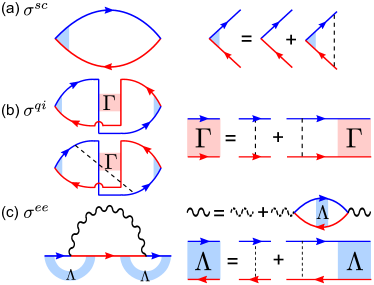
Figure 1: The Feynman diagrams McCann et al. (2006); Altshuler et al. (1980); Fukuyama (1980); Lee and Ramakrishnan (1985); Lu et al. (2011); Shan et al. (2012); Lu and Shen (2014) for the conductivity of 3D Weyl semimetals, in the presence of disorder (dashed lines) and electron-electron interaction (wavy lines). The arrow lines are for Green’s functions.

III Finite-temperature conductivity

III.1 Quantum interference and weak antilocalization

According to the classification of random ensembles Dyson (1962), systems with time-reversal symmetry but broken spin-rotational symmetry are classified into the symplectic class. A symplectic system is supposed to exhibit the weak antilocalization effect Hikami et al. (1980), when the quantum interference [see Fig. 1(b)] corrects the conductivity. Weyl fermions in a single valley have the symplectic symmetry so the weak antilocalization effect is expected. We find that the quantum interference correction for one valley of Weyl fermions takes the form (detailed calculation in Sec. VIII)

$$\sigma^{qi}(T)=\frac{e^{2}}{h}\frac{1}{\pi^{2}}(\frac{1}{\ell}-\frac{1}{\ell_{\phi}}),$$ (2)

where $e^{2}/h$ is the conductance quantum, $\ell$ is the mean free path, and $\ell_{\phi}$ is the phase coherence length. This single-valley result has exactly the same magnitude but opposite sign compared to that for conventional 3D electrons (with dispersion $(\hbar k)^{2}/2m$) per spin Lee and Ramakrishnan (1985). With decreasing temperature, $\ell_{\phi}$ always increases as decoherence induced by inelastic scattering is suppressed gradually. Therefore, $\sigma^{qi}$ will be enhanced when lowering the temperature, literally giving a weak antilocalization contribution (see $\sigma^{qi}$ in Fig. 2). The temperature dependence of $\sigma^{qi}$ is from $\ell_{\phi}=CT^{-p/2}$ Thouless (1977), where $C$ is a constant and $p$ depends only on dimensionality and decoherence mechanisms thus does not distinguish conventional systems and Weyl semimetals. In 3D, $p=3/2$ ($p=3$) if electron-electron (electron-phonon) interaction is the decoherence mechanism in the disordered limit Lee and Ramakrishnan (1985). Also, because our calculation is in 3D, the functional relationship is not logarithmic as that in quasi-2D Garate and Glazman (2012); Lu and Shen (2011). For Weyl semimetals realized by breaking time-reversal symmetry Xu et al. (2011), the weak antilocalization may be suppressed by magnetism.

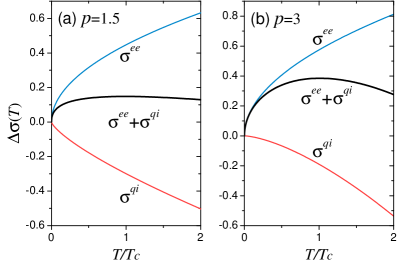
Figure 2: A schematic demonstration of the change of conductivity $\Delta\sigma$ as a function of temperature $T$. We choose $c_{ee}=c_{qi}$. $T_{c}$ is the critical temperature below which the conductivity drops with decreasing temperature.

III.2 Weak localization induced by the interplay of interaction and disorder

Despite the signature in magnetoconductivity, we will show that the weak antilocalization breaks down in the presence of many-body interactions. The dominant interaction correction to the conductivity is attributed to the one-loop Fock (exchange interaction) self-energy dressed by Diffusons [see Fig. 1(c)]. We find that, for Weyl fermions, this self-energy gives a correction of the same form as that for conventional 3D electrons, upon a redefinition of the parameters such as the diffusion coefficient $D$. Besides the self-energy in Fig. 1(c), there are three other one-loop self-energies (see Fig. 10). These four self-energies contribute to a correction to the conductivity

$$\sigma^{ee}(T)\approx\frac{e^{2}}{h}(1-F)\sqrt{\frac{k_{B}T}{\hbar D}}\times 0.195,$$ (3)

where $k_{B}$ is the Boltzmann constant and the screening factor $F$ is defined as the average of the interaction over the Fermi surface. In 3D, $F=[\ln(1+x)]/x$ Lee and Ramakrishnan (1985), where we find $x=8\pi^{2}v_{F}\hbar\varepsilon/e^{2}$ for Weyl fermions, with $\varepsilon$ the dielectric constant. By definition, $F\in[0,1]$, as shown in Table 1 for several popular candidates of Weyl semimetal. Therefore, $\sigma^{ee}$ decreases with decreasing temperature following a law of $\sqrt{T}$, giving a localization tendency. Disorder is inevitable in realistic materials so here the interaction is dressed by disorder, while in the clean limit the interaction alone may give a linear-$T$ conductivity Goswami and Chakravarty (2011); Hosur et al. (2012). In the clean limit, a marginal Fermi liquid phase and generation of mass are found for Dirac semimetals González (2014). Also, $F$ will be further corrected to $\widetilde{F}$ after including the second-order interaction self-energies and interaction correction to the disorder scattering Lee and Ramakrishnan (1985). However $\widetilde{F}\sim F$ and $\widetilde{F}\leq F$ (see Tab. 1 and Fig. 13). Later, we will see that there is always a localization tendency as long as $1-F>0$, where the dominant 1 is contributed by the self-energy in Fig. 1(c). The interaction part $\sigma^{ee}$ also contributes to a negative magnetoconductivity, with a magnitude much smaller than $\delta\sigma^{qi}(B)$, this property is consistent with conventional electrons Lee and Ramakrishnan (1985).

Table 1: The dielectric constant $\varepsilon$ (in units of vacuum dielectric constant), Fermi velocity $v_{F}$, and screening factor $F$ and $\widetilde{F}$ (after the renormalization) for several candidates of Weyl semimetals. Because of anisotropy, $v_{F}\hbar$ covers a wide range in Bi_0.97Sb_0.03 and Cd₃As₂.

	$\varepsilon$	$v_{F}\hbar$ [eV$\cdot$Å]	$F$	$\widetilde{F}$
Bi0.97Sb0.03	100	1-10	0.09-0.01	0.09-0.01
Refs.	[Boyle and Brailsford, 1960]	[Golin, 1968,Liu and Allen, 1995]
TlBiSSe	20	1.1	0.25	0.24
Refs.	[Novak et al., 2015]	[Novak et al., 2015]
Cd3As2	36-52	2-7	0.03-0.11	0.03-0.11
Refs.	[Cisowski and Bodnar, 1975; Jay-Gerin et al., 1977; Blom and Gelten, 1977]	[Wang et al., 2013,Borisenko et al., 2014]

III.3 Competing weak antilocalization and localization

Combining $\sigma^{qi}$ and $\sigma^{ee}$, the change of conductivity with temperature for one valley of Weyl fermions can be summarized as

$$\Delta\sigma(T)=c_{ee}T^{1/2}-c_{qi}T^{p/2},$$ (4)

where $c_{ee}=0.195(1-F)\sqrt{k_{B}/\hbar D}$ and $c_{qi}=1/c\pi^{2}$ in units of $e^{2}/h$. This describes a competition between the interaction-induced weak localization and interference-induced weak antilocalization, as shown in Fig. 2 schematically. At higher temperatures, the conductivity increases with decreasing temperature, showing a weak antilocalization behavior. Below a critical temperature $T_{c}$, the conductivity starts to drop with decreasing temperature, exhibiting a localization tendency. From $\partial\Delta\sigma/\partial T=0$, the critical temperature can be found as $T_{c}=\left(c_{ee}/p\cdot c_{qi}\right)^{2/(p-1)}$, at which $\left.(\partial^{2}\Delta\sigma/\partial T^{2})\right|_{T_{c}}\approx(1-p)(p\cdot c_{qi}/4)\left(c_{ee}/p\cdot c_{qi}\right)^{(p-4)/(p-1)}$. Because $c_{ee},c_{qi}>0$, this means as long as $p>1$, there is always a critical temperature, below which the conductivity drops with decreasing temperature. For known decoherence mechanisms in 3D, $p$ is always greater than 1 Lee and Ramakrishnan (1985). Now we estimate the critical temperature $T_{c}$. Using $c_{ee}$ and $c_{qi}$, we arrive at $T_{c}\approx\left[C(1-F)/(2p\sqrt{v_{F}\ell})\right]^{2/(p-1)}$, which shows that $T_{c}$ increases with $C$ while decreases with $F$, $p$, $v_{F}$, and $\ell$. With a set of typical parameters $F=0.25\sim 0.01$ and $v_{F}=10\sim 1\times 10^{5}$ m/s, as well as $p=3\sim 3/2$, $C=100\sim 1000$ nm$\cdot$K^p/2, $\ell=100\sim 10$ nm in disordered metals, we find that $T_{c}\approx 0.4\sim 10^{6}$ K. Please note that our calculation is not justified at high temperatures, but in this way we show that the localization tendency is experimentally accessible in disordered Weyl semimetals. For Cd₃As₂ with extremely high mobility, the recent experiment Liang et al. (2015) demonstrated that the mean free path $\ell$ is well above 1 $\mu$m, yielding a $T_{c}$ well below those achievable (10 mK) in most laboratories. To summarize the transport properties of a single valley of Weyl fermions, Table 3 compares them with those of 2D massless Dirac fermions and 3D conventional electrons.

IV Magnetoconductivity

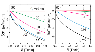
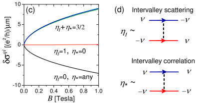
Figure 3: The magnetoconductivity $\delta\sigma^{qi}(B)$ for different phase coherence length $\ell_{\phi}$ at $\eta_{I}=\eta_{*}=0$ (a), for different $\eta_{I}$ at $\eta_{*}=0$ (b), and for different $\eta_{I}$ at finite $\eta_{*}$ (c). Parameters: $\ell=10$ nm and $\ell_{\phi}=1000$ nm in (b) and (c). (d) The diagrams show the difference between $\eta_{I}$ and $\eta_{*}$, with $\eta_{I}$ related to the intervalley scattering and $\eta_{*}$ measuring the intervalley correlation of intravalley scattering. The dashed lines represent the correlation of two scattering processes. $\nu=\pm$ is the valley index.

IV.1 The $-\sqrt{B}$ magnetoconductivity of a single valley of Weyl fermions

Because of its quantum interference origin, $\sigma^{qi}$ in Eq. (2) can be suppressed by a magnetic field, giving rise to a magnetoconductivity $\delta\sigma^{qi}(B)\equiv\sigma^{qi}(B)-\sigma^{qi}(0)$, where

$$\sigma^{qi}(B)=\frac{2e^{2}}{h}\int_{0}^{1/\ell}\frac{dx}{(2\pi)^{2}}$$

$$\times\left[\psi\left(\frac{\ell_{B}^{2}}{\ell^{2}}+\ell_{B}^{2}x^{2}+\frac{1}{2}\right)-\psi\left(\frac{\ell_{B}^{2}}{\ell_{\phi}^{2}}+\ell_{B}^{2}x^{2}+\frac{1}{2}\right)\right]$$ (5)

for one valley of Weyl fermions, with $\psi$ the digamma function and $\ell_{B}\equiv\sqrt{\hbar/4eB}$ the magnetic length. The magnetic field $B$ is applied along arbitrary directions (we have checked that $\sigma_{xx}^{qi}=\sigma_{zz}^{qi}$). As $B\rightarrow\infty$, $\delta\sigma^{qi}$ saturates following a $1/B$ dependence. As $B\rightarrow 0$, $\delta\sigma^{qi}$ is proportional to $-\sqrt{B}$ for $\ell_{\phi}\gg\ell_{B}$ or at low temperatures, and $\delta\sigma^{qi}\propto-B^{2}$ for $\ell_{\phi}\ll\ell_{B}$ at high temperatures. $\ell_{B}$ can be evaluated approximately as 12.8 nm$/\sqrt{B}$ with $B$ in Tesla. Usually below the liquid helium temperature, $\ell_{\phi}$ can be as long as hundreds of nanometers to one micrometer, much longer than $\ell_{B}$ which is tens of nanometers between 0.1 and 1 Tesla. Therefore, the $-\sqrt{B}$ magnetoconductivity at low temperatures and small fields serves as a signature for the weak antilocalization of 3D Weyl fermions. Fig. 3(a) shows $\delta\sigma^{qi}(B)$ of two valleys of Weyl fermions in the absence of intervalley scattering. For long $\ell_{\phi}$, $\delta\sigma^{qi}(B)$ is negative and proportional to $\sqrt{B}$, showing the signature of the weak antilocalization of 3D Weyl fermions. This $-\sqrt{B}$ dependence agrees well with the experiment Kim et al. (2013, 2014), and we emphasize that it is obtained from a complete diagram calculation with only two parameters $\ell$ and $\ell_{\phi}$ of physical meanings. As $\ell_{\phi}$ becomes shorter, a change from $-\sqrt{B}$ to $B^{2}$ is evident. $\delta^{qi}(B)$ vanishes at $\ell_{\phi}=\ell$ as the system quits the quantum interference regime. Also, it is known that the chiral anomaly could give a positive magnetoconductivity Son and Spivak (2013); Kim et al. (2014); Burkov (2014); Gorbar et al. (2014), competing with the negative magnetoconductivity from the weak antilocalization. This chiral-anomaly part, because of its $B^{2}$ dependence, will always be overwhelmed by the $-\sqrt{B}$ weak antilocalization part at weak magnetic fields. At high fields, the chiral anomaly may become dominant.

IV.2 Weak localization induced by inter-valley effects

Now we come to consider the effects of intervalley scattering and correlation. We will focus on the quantum interference part and magnetoconductivity [see Sec. VIII.3 for the expressions of $\sigma^{qi}$ and $\delta\sigma^{qi}(B)$ in the presence of intervalley scattering and correlation], because we find that the interaction brings a negligible valley-dependent effect. Two dimensionless parameters are defined for the inter- and intravalley scattering: $\eta_{*}\propto\langle U_{\mathbf{k},\mathbf{k}^{\prime}}^{++}U_{\mathbf{k}^{\prime},\mathbf{k}}^{--}\rangle$ measuring the correlation between intravalley scattering and $\eta_{I}\propto\langle U_{\mathbf{k},\mathbf{k}^{\prime}}^{+-}U_{\mathbf{k}^{\prime},\mathbf{k}}^{-+}\rangle$ measuring the weight of intervalley scattering , where $U_{\mathbf{k},\mathbf{k}^{\prime}}^{\nu,\nu^{\prime}}$ is the scattering matrix element. Figure 3(d) schematically shows the difference between $\eta_{*}$ and $\eta_{I}$. As shown in Fig. 3(b), with increasing $\eta_{I}$, the negative $\delta\sigma^{qi}$ is suppressed, where $\eta_{I}\rightarrow 1$ means strong intervalley scattering while $\eta_{I}\rightarrow 0$ means vanishing intervalley scattering. Furthermore, Fig. 3(c) shows that the magnetoconductivity can turn to positive when $\eta_{I}+\eta_{*}=3/2$. Remember that the negative $\delta\sigma^{qi}(B)$ in Fig. 3(b) is related to the increasing $\sigma^{qi}(T)$ with decreasing $T$ in Fig. 2, as two signatures of the weak antilocalization. Similarly, the positive $\delta\sigma^{qi}(B)$ in Fig. 3(c) corresponds to a suppressed $\sigma^{qi}$ with decreasing temperature, i.e., a localization tendency. This localization is attributed to the strong intervalley coupling which recovers spin-rotational symmetry (now the spin space is complete for a given momentum), then the system goes to the orthogonal class Dyson (1962); Hikami et al. (1980); Suzuura and Ando (2002). Therefore, we show that the combination of strong intervalley scattering and correlation will strengthen the localization tendency in disordered Weyl semimetals.

IV.3 Comparison with magnetoconductivity in experiments

Table 2: Comparison between the classical magnetoconductivity (MC) induced by the Lorentz force $\delta\sigma^{C}(B)$, semiclassical MC induced by the chiral anomaly $\delta\sigma^{A}(B)$ Son and Spivak (2013); Burkov (2014), and weak antilocalization MC induced by the quantum interference $\delta\sigma^{qi}(B)$, in their dependences on magnetic field $B$, temperature $T$, Fermi wave vector $k_{F}$, and mean free path $\ell$, in the limit $\eta_{I}\rightarrow 0$.

Dependence	$\delta\sigma^{C}$	$\delta\sigma^{A}$	$\delta\sigma^{qi}(\eta_{I}\rightarrow 0)$
$B$	$-B^{2}$	$B^{2}$	$-\sqrt{B}$
$B$ direction	$\perp$	$||$	Any
$T$	No	No	Suppressed with increasing $T$
$k_{F}$	No	$1/k_{F}^{2}$	No
$\ell$	$\ell^{3}$	$\ell$	Decreases with increasing $\ell$
$\eta_{I}$	No	$1/\eta_{I}$	Suppressed with increasing $\eta_{I}$

To compare with experiments, besides the magnetoconductivity $\delta\sigma^{qi}(B)$ arising from the weak antilocalization in Sec. IV.1, two more contributions to the total magnetoconductivity have to be taken into account. One is the classical negative magnetoconductivity due the cyclotron motion of electron driven by the Lorentz force in perpendicular magnetic fields and is given by $\delta\sigma^{C}=-\sigma^{sc}\mu^{2}B^{2}$ Datta (1997), where for the Weyl fermion the mobility is given by $\mu=ev_{F}\tau\eta_{v}/\hbar k_{F}$, then (see Sec. X for details)

$$\delta\sigma^{C}(B)=-\frac{e^{2}}{h}\frac{\sqrt{3}\eta_{v}^{3/2}}{16\pi}\frac{\ell^{3}}{\ell_{B}^{4}}.$$ (6)

This part arises only in a perpendicular field and is not a function of $k_{F}$. It becomes dominant for long $\ell$, i.e., in high-mobility and clean samples.

The other semiclassical magnetoconductivity is from the chiral anomaly, which arises because of the nontrivial Berry curvature carried by Weyl fermions, and it can give a magnetic field dependent correction to the velocity and Drude conductivity. An explicit form of $\delta\sigma^{A}(B)$ has been derived by Son and Spivak Son and Spivak (2013) and Burkov Burkov (2014). For example, according to Burkov Burkov (2014)

$$\delta\sigma^{A}(B) = \frac{e^{4}B^{2}\tau_{a}}{4\pi^{4}g(E_{F})}$$ (7)

where $\hbar=1$, $g(E_{F})=2N_{F}$. $\tau_{a}$ is referred to as the axial relaxation time, which is supposed to be an independent parameter. Here, we use the intervalley scattering time for the axial relaxation time. In terms of the notations used in this work

$$\delta\sigma^{A}(B)=\frac{e^{2}}{h}\frac{\ell}{\ell_{B}^{4}}\frac{1}{k_{F}^{2}}\frac{\sqrt{2(1+\eta_{I})}}{32\pi\eta_{I}}.$$ (8)

Here $\ell_{B}\equiv\sqrt{\hbar/4eB}$. The Berry curvature correction may also be the reason for some anomalous magnetoconductivity in topological insulators Wang et al. (2012b).

Including the three contributions, now the total magnetoconductivity is

$$\delta\sigma_{||}(B) = \delta\sigma^{qi}(B)+\delta\sigma^{A}(B)$$ (9)

when the current is parallel to the magnetic field, and

$$\delta\sigma_{\perp}(B) = \delta\sigma^{qi}(B)+\delta\sigma^{C}(B)$$ (10)

when the current is perpendicular to the magnetic field.

In Table 2, we compare these three different magnetoconductivity. Please note that, $\delta\sigma^{C}$ dominates in clean samples because it is proportional to $\ell^{3}$ while $\delta\sigma^{A}$ dominates near Weyl nodes because it is proportional to $1/k_{F}^{2}$, and $\delta\sigma^{qi}$ appear only at low temperatures.

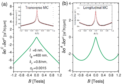
Figure 4: Comparison with the experimental magnetoconductivity by Kim et al. (insets) Kim et al. (2013). The transverse magnetoconductivity (MC) $\delta\sigma_{\perp}(B)=\delta\sigma^{C}+\delta\sigma^{qi}$ and longitudinal MC $\delta\sigma_{||}(B)=\delta\sigma^{A}+\delta\sigma^{qi}$ are defined when the current is perpendicular and parallel to the magnetic field, respectively. The classical MC induced by the Lorentz force $\delta\sigma^{C}(B)$ is given in Eq. (6). The semiclassical MC induced by the chiral anomaly $\delta\sigma^{A}(B)$ Son and Spivak (2013); Burkov (2014) is in Eq. (8). The delocalization MC induced by the quantum interference $\delta\sigma^{qi}(B)$ is in Sec. (VIII.3).

In Fig. 4, we use Eqs. (9) and (10) to reproduce the magnetoconductivity measured by Kim et al. in Bi_0.03Sb_0.97 Kim et al. (2013). The main features (e.g., the transverse MC is several times of the longitudinal MC, those inflection points in MC) in both the transverse and longitudinal magnetoconductivity can be recovered simultaneously within a set of parameters comparable to those in relevant materials. Our parameters (e.g., mean free path, Fermi wave vector) are of physical meanings. Figure 4 (a) is always negative because both $\delta\sigma^{C}$ and $\delta\sigma^{qi}$ are negative. The competition between $\delta\sigma^{qi}\propto-\sqrt{B}$ and $\delta\sigma^{A}\propto B^{2}$ leads to the inflection in Fig. 4 (b).

V Comparison of Weyl fermions, 2D Dirac fermions, and 3D conventional electrons

To summarize, we compare the transport properties for single valley of Weyl Fermions, 2D massless Dirac fermions, and 3D conventional electrons, in Table 3.

Table 3: Comparison between a single valley of 2D massless Dirac fermions Suzuura and Ando (2002); McCann et al. (2006), a single valley of 3D Weyl fermions, and a single band of 3D conventional electrons Altshuler et al. (1980); Fukuyama (1980). $k_{F}$ is the Fermi wave vector, $m$ is the effective mass, $v_{F}$ is the constant Fermi velocity of Dirac and Weyl fermions, $\tau$ is the total momentum relaxation time, and $\eta_{v}$ is the correction to the velocity (Sec. VII). $\eta_{I}\in[0,1]$ measures the weight of intervalley scattering. $F$ is the screening factor of interaction (Sec. IX.3). $\varepsilon$ is the dielectric constant. $\sigma^{ee}$ is the conductivity correction from the interplay of electron-electron interaction and disorder scattering. $\sigma^{qi}$ is the conductivity correction from the quantum interference. $\delta\sigma^{qi}(B)$ is the small-field magnetoconductivity from $\sigma^{qi}$ when $\ell_{\phi}\gg\ell_{B}$. $p$ is the exponent in the temperature dependence of the phase coherence length Thouless (1977) $\ell_{\phi}\sim T^{-p/2}$ due to electron-electron interaction (EEI) and electron-phonon (E-Ph) interaction in disordered metals Lee and Ramakrishnan (1985).

	2D massless Dirac	3D Weyl	3D Conventional
Dispersion $E(\mathbf{k})$	$\pm\gamma\sqrt{k_{x}^{2}+k_{y}^{2}}$	$\pm\gamma\sqrt{k_{x}^{2}+k_{y}^{2}+k_{z}^{2}}$	$(\hbar^{2}/2m)(k_{x}^{2}+k_{y}^{2}+k_{z}^{2})$
Density of states $N(E)$	$E/2\pi(v_{F}\hbar)^{2}$	$E^{2}/2\pi^{2}(v_{F}\hbar)^{3}$	$(1/2\pi)^{2}(2m/\hbar^{2})^{3/2}\sqrt{E}$
Carrier density per valley	$k_{F}^{2}/4\pi$	$k_{F}^{3}/6\pi^{2}$	$k_{F}^{3}/6\pi^{2}$
Mobility $\mu$	$ev_{F}\tau\eta_{v}/\hbar k_{F}$	$ev_{F}\tau\eta_{v}/\hbar k_{F}$	$e\tau/m$
Diffusion coefficient $D$	$v_{F}^{2}\tau\eta_{v}/2$	$v_{F}^{2}\tau\eta_{v}/3$	$(\hbar k_{F}/m)^{2}\tau/3$
Velocity correction $\eta_{v}$	2 Shon and Ando (1998)	3/2 Garate and Glazman (2012); Biswas and Ryu (2014)	1
		$(3/2)/(1+\eta_{I})$
$\eta_{H}$	-1/4 McCann et al. (2006)	-1/6 Garate and Glazman (2012)	0
Screening factor $F$	$(2/\pi)(\arctan\sqrt{1/x^{2}-1})/\sqrt{1-x^{2}}$	$[\ln(1+x)]/x$	$[\ln(1+x)]/x$
	$x=8\pi\varepsilon v_{F}\hbar/e^{2}$	$x=8\pi^{2}\varepsilon v_{F}\hbar/e^{2}$	$x=8\pi^{2}\varepsilon\hbar^{2}k_{F}/me^{2}$
$\delta\sigma^{qi}(B\rightarrow 0)\propto$	$-B$	$-\sqrt{B}$	$\sqrt{B}$ Kawabata (1980)
$\sigma^{ee}(T)\propto$	$\ln T$ Lu and Shen (2014); Liu et al. (2014c)	$\sqrt{T}$	$\sqrt{T}$ Altshuler et al. (1980); Fukuyama (1980)
$\sigma^{qi}(T)\propto$	$-\ln T$ Suzuura and Ando (2002); McCann et al. (2006)	$-T^{p/2}$	$T^{p/2}$ Altshuler et al. (1980); Fukuyama (1980)
$p$ (EEI) Lee and Ramakrishnan (1985)	1	3/2	3/2
$p$ (E-Ph) Lee and Ramakrishnan (1985)	3	3	3

VI The Calculation of the conductivity

Throughout the work, we will only focus on the conductivity of the conduction bands. The valence bands have the same properties. The eigen energies of the conduction bands in the two valleys are degenerate

$$E_{\mathbf{k}}=v_{F}\hbar k=v_{F}\hbar\sqrt{k_{x}^{2}+k_{y}^{2}+k_{z}^{2}},$$ (11)

where $\mathbf{k}$ is measured from each Weyl node. The spinor wave function of the conduction band in valley $+$ is

$$|+,\mathbf{k}\rangle=\left(\begin{array}[]{c}\cos\frac{\theta}{2}\\ \sin\frac{\theta}{2}e^{i\varphi}\\ \end{array}\right)\frac{e^{i\mathbf{k}\cdot\mathbf{r}}}{\sqrt{\Omega}},$$ (14)

where $\theta$ and $\varphi$ are the wave vector angles, $\tan\varphi\equiv k_{y}/k_{x}$, $\cos\theta\equiv k_{z}/k$, and $\Omega$ is the volume. In valley $-$, the wave function of the conduction band can be found as ($\theta\rightarrow\pi-\theta$ and $\varphi\rightarrow\pi+\varphi$),

$$|-,\mathbf{k}\rangle=\left(\begin{array}[]{c}\sin\frac{\theta}{2}\\ -\cos\frac{\theta}{2}e^{i\varphi}\\ \end{array}\right)\frac{e^{i\mathbf{k}\cdot\mathbf{r}}}{\sqrt{\Omega}}.$$ (17)

The total conductivity has three dominant parts

$$\sigma = \sigma^{sc}+\sigma^{qi}+\sigma^{ee}.$$ (18)

$\sigma^{sc}$ is the semiclassical conductivity (Sec. VII), $\sigma^{qi}$ is the correction from the quantum interference (Sec. VIII), and $\sigma^{ee}$ is the correction from the interplay of electron-electron interaction and disorder scattering (Sec. IX).

VII Semiclassical (Drude) conductivity

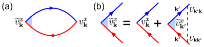
Figure 5: (a) The Feynman diagram for the semiclassical (Drude) conductivity $\sigma^{sc}$. (b) The diagram for the vertex correction to the velocity Shon and Ando (1998). $v$ is the velocity. The arrow lines are for Green’s functions. The dashed lines are for disorder scattering ($U$). Replace $x$ by $z$ for the conductivity along the $z$ direction.

The semiclassical (Drude) conductivity can be found as [see Fig. 5(a)]

$$\sigma^{sc}=\frac{e^{2}\hbar}{2\pi}\sum_{\mathbf{k}}v^{i}_{\mathbf{k}}G^{\mathrm{R}}_{\mathbf{k}}G^{\mathrm{A}}_{\mathbf{k}}\widetilde{v}^{i}_{\mathbf{k}},$$ (19)

where $i=x$ or $z$, $G^{R/A}$ is the retarded/advanced Green’s function, $v^{i}_{\mathbf{k}}=(1/\hbar)\partial_{i}/\partial E_{\mathbf{k}}$ is the velocity, and $\widetilde{v}^{i}_{\mathbf{k}}$ is the corrected velocity by the disorder scattering [see Fig. 5 (b)]. The retarded (R) and advanced (A) Green’s functions

$$G^{\mathrm{R/A}}_{\mathbf{k}}(\omega) = \frac{1}{\omega-\xi_{\mathbf{k}}\pm i\frac{\hbar}{2\tau}},$$ (20)

where $\xi_{\mathbf{k}}=E_{\mathbf{k}}-E_{F}$. The total scattering time (or total momentum relaxation time) $\tau$ is defined as

$$\frac{1}{\tau}\equiv\frac{1}{\tau_{0}}+\frac{1}{\tau_{I}},$$ (21)

where the intra- and inter-valley scattering times are given by

$$\frac{1}{\tau_{0}} \equiv \frac{2\pi}{\hbar}\sum_{\mathbf{k}^{\prime}}\langle|U^{++}_{\mathbf{k},\mathbf{k}^{\prime}}|^{2}\rangle\delta(E_{F}-\xi_{\mathbf{k}^{\prime}})=\frac{2\pi}{\hbar}N_{F}\frac{nu_{0}^{2}}{2},$$

$$\frac{1}{\tau_{I}} \equiv \frac{2\pi}{\hbar}\sum_{\mathbf{k}^{\prime}}\langle|U^{+-}_{\mathbf{k},\mathbf{k}^{\prime}}|^{2}\rangle\delta(E_{F}-\xi_{\mathbf{k}^{\prime}})=\frac{2\pi}{\hbar}N_{F}\frac{nu_{I}^{2}}{2},$$ (22)

$n$ is the impurity density, $u_{0}$ and $u_{I}$ measure the strength for the intra- and inter-valley scattering, respectively. $N_{F}=E_{F}^{2}/2\pi^{2}(v_{F}\hbar)^{3}$ is the density of states per valley. $U_{\mathbf{k},\mathbf{k}^{\prime}}^{++}\equiv\langle+,\mathbf{k}|U(\mathbf{r})|+,\mathbf{k}^{\prime}\rangle$ and $U_{\mathbf{k},\mathbf{k}^{\prime}}^{+-}\equiv\langle+,\mathbf{k}|U(\mathbf{r})|-,\mathbf{k}^{\prime}\rangle$ are the intravalley and intervalley scattering matrix elements, respectively, and

$$U^{++}_{\mathbf{k},\mathbf{k}^{\prime}} = \sum_{i}u_{i}e^{i(\mathbf{k}^{\prime}-\mathbf{k})\cdot\mathbf{R}_{i}}[aa^{\prime}+bb^{\prime}e^{i(\varphi^{\prime}-\varphi)}],$$

$$U^{+-}_{\mathbf{k},\mathbf{k}^{\prime}} = \sum_{i}u_{i}e^{i(\mathbf{k}^{\prime}-\mathbf{k})\cdot\mathbf{R}_{i}}[ab^{\prime}-ba^{\prime}e^{i(\varphi^{\prime}-\varphi)}],$$ (23)

with $a\equiv\cos(\theta/2)$ and $b\equiv\sin(\theta/2)$.

The correction to the velocity can be found from the iteration equation [see Fig. 5(b)]

$$\widetilde{v}^{i}_{\mathbf{k}} = v^{i}_{\mathbf{k}}+\sum_{\mathbf{k}^{\prime}}G^{\mathrm{R}}_{\mathbf{k}^{\prime}}G^{\mathrm{A}}_{\mathbf{k}^{\prime}}\langle U_{\mathbf{k},\mathbf{k}^{\prime}}U_{\mathbf{k}^{\prime},\mathbf{k}}\rangle\widetilde{v}^{i}_{\mathbf{k}^{\prime}}.$$ (24)

In polar coordinates, $v^{x}_{\mathbf{k}}=v_{F}\sin\theta\cos\varphi$ and $v_{\mathbf{k}}^{z}=v_{F}\cos\theta$,

$$\int_{0}^{\infty}(k^{\prime})^{2}\frac{dk^{\prime}}{2\pi}G^{\mathrm{R}}_{\mathbf{k}^{\prime}}G^{\mathrm{A}}_{\mathbf{k}^{\prime}} \approx \frac{2\pi^{2}N_{F}\tau}{\hbar},$$ (25)

and

$$\langle U_{\mathbf{k},\mathbf{k}^{\prime}}U_{\mathbf{k}^{\prime},\mathbf{k}}\rangle=\langle U^{++}_{\mathbf{k},\mathbf{k}^{\prime}}U^{++}_{\mathbf{k}^{\prime},\mathbf{k}}\rangle+\langle U^{+-}_{\mathbf{k},\mathbf{k}^{\prime}}U^{-+}_{\mathbf{k}^{\prime},\mathbf{k}}\rangle$$

$$\approx\frac{\hbar}{2\pi N_{F}\tau}[1+(1-2\eta_{I})$$

$$\times(\cos\theta\cos\theta^{\prime}+\sin\theta\sin\theta^{\prime}\cos(\varphi-\varphi^{\prime}))],$$ (26)

where $\eta_{I}\equiv\tau/\tau_{I}$ and $1/\tau\equiv 1/\tau_{0}+1/\tau_{I}$, and $\tau_{0}$ and $\tau_{I}$ are the intravalley and intervalley scattering times, respectively. So $\eta_{I}\in[0,1]$ measures the relative strength of intervalley scattering. By assuming $\widetilde{v}^{x}_{\mathbf{k}}=\eta_{v}v_{\mathbf{k}}^{x}$ and $\widetilde{v}^{z}_{\mathbf{k}}=\eta_{v}v_{\mathbf{k}}^{z}$, and put them into the iteration equation for the velocity, one can readily find that for either the velocity along $x$ or $z$ direction

$$\eta_{v} = \frac{3}{2(1+\eta_{I})}.$$ (27)

Finally, we found that for either $x$ and $z$ direction,

$$\sigma^{sc} = e^{2}N_{F}\frac{1}{3}v_{F}^{2}\tau\eta_{v},$$ (28)

where the density of states per valley $N_{F}=E_{F}^{2}/2\pi^{2}(v_{F}\hbar)^{3}$. It satisfies the Einstein relation

$$\sigma^{sc} = e^{2}N_{F}D,$$ (29)

with the diffusion coefficient $D\equiv v_{F}^{2}\tau\eta_{v}/d$, where $d=3$ for three dimensions. Usually, $\tau\eta_{v}$ is referred to as the transport time. Later, we will show that $D$ can also be derived from the calculation of the Diffuson (Sec. IX.1).

In terms of the mean free path $\ell\equiv\sqrt{D\tau}$ and Fermi wave vector $k_{F}$,

$$\sigma^{sc} = \frac{e^{2}}{h}\frac{k_{F}^{2}\ell}{\pi}\sqrt{\frac{\eta_{v}}{3}}=\frac{e^{2}}{h}\frac{k_{F}^{2}\ell}{\pi\sqrt{2(1+\eta_{I})}}.$$ (30)

VIII Conductivity correction from quantum interference

The total conductivity from the quantum interference has two parts

$$\sigma^{qi} = 2\times\sigma^{qi}_{0}+\sigma^{qi}_{I}.$$ (31)

$\sigma^{qi}_{0}$ is from the intravalley Cooperons (Sec. VIII.1) and $\sigma^{qi}_{I}$ is from the intervalley Cooperons (Sec. VIII.2).

VIII.1 Conductivity correction from intravalley Cooperons

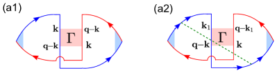
Figure 6: The Feynman diagrams for the quantum interference correction to the conductivity that take into account the Cooperons from only the intravalley scattering. These diagrams give $\sigma^{qi}_{0}$.

The conductivity contribution from the intravalley Cooperons is given by (see Fig. 6)

$$\sigma^{qi}_{0}=\sigma_{a1}+2\times\sigma_{a2},$$ (32)

where

$$\sigma_{a1} = \frac{e^{2}\hbar}{2\pi}\sum_{\mathbf{q}}\Gamma_{\mathbf{k},\mathbf{q}-\mathbf{k}}\sum_{\mathbf{k}}G^{R}_{\mathbf{k}}\widetilde{v}^{x}_{\mathbf{k}}G^{A}_{\mathbf{k}}G^{R}_{\mathbf{q-k}}\widetilde{v}^{x}_{\mathbf{q-k}}G^{A}_{\mathbf{q-k}},$$

$$\sigma_{a2} = \frac{e^{2}\hbar}{2\pi}\sum_{\mathbf{q}}\Gamma_{\mathbf{k}_{1},\mathbf{q}-\mathbf{k}}\sum_{\mathbf{k}}\sum_{\mathbf{k}_{1}}\widetilde{v}^{x}_{\mathbf{k}}\widetilde{v}^{x}_{\mathbf{q}-\mathbf{k}_{1}}G^{R}_{\mathbf{k}}G^{R}_{\mathbf{k}_{1}}G^{R}_{\mathbf{q}-\mathbf{k}}$$ (33)

$$\times G^{R}_{\mathbf{q}-\mathbf{k}_{1}}G^{A}_{\mathbf{k}}G^{A}_{\mathbf{q}-\mathbf{k}_{1}}\langle U_{\mathbf{k},\mathbf{k}_{1}}U_{\mathbf{q}-\mathbf{k},\mathbf{q}-\mathbf{k}_{1}}\rangle.$$

We also find that the ratio of the dressed to bare Hikami boxes is

$$\eta_{H}\equiv\frac{\sigma_{a2}}{\sigma_{a1}}=-\frac{1}{6},$$ (34)

consistent with that by Garate and Glazman Garate and Glazman (2012).

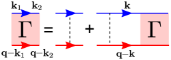
Figure 7: The Feynman diagram of the Bethe-Salpeter equation for the intravalley Cooperons. The valley index is suppressed because the valley is conserved during the scattering.

In polar coordinates, the intra-valley Cooperon can be found by the Bethe-Salpeter equation (see Fig. 7)

$$\Gamma_{\mathbf{k}_{1},\mathbf{k}_{2}} = \Gamma_{\mathbf{k}_{1},\mathbf{k}_{2}}^{0}+\int_{0}^{2\pi}\frac{d\varphi}{2\pi}\int_{0}^{\pi}\frac{d\theta\sin\theta}{2\pi}\int_{0}^{\infty}\frac{dkk^{2}}{2\pi}$$ (35)

$$\times\Gamma_{\mathbf{k}_{1},\mathbf{k}}^{0}\mathcal{G}_{\mathbf{k}}^{i\epsilon_{n}}\mathcal{G}_{\mathbf{q-k}}^{i\epsilon_{n}-i\omega_{m}}\Gamma_{\mathbf{k},\mathbf{k}_{2}},$$

where the Matsubara Green’s function is given as

$$\mathcal{G}(\mathbf{k},i\epsilon_{n}) = \frac{1}{i\hbar\epsilon_{n}-\xi_{\mathbf{k}}+i\frac{\hbar}{2\tau}\mathrm{sgn}(\epsilon_{n})},$$ (36)

the fermionic Matsubara frequency $\epsilon_{n}=(2n+1)\pi k_{B}T/\hbar$ with $n=0,\pm 1,\pm 2,...$, the bosonic Matsubara frequency $\omega_{m}=2\pi mk_{B}T/\hbar$ with $m=0,\pm 1,\pm 2,...$, and $\xi_{\mathbf{k}}=E_{\mathbf{k}}-E_{F}$ with $E_{F}$ the Fermi energy. The bare Cooperon

$$\Gamma_{\mathbf{k}_{1},\mathbf{k}_{2}}^{0}\equiv\langle U_{\mathbf{k}_{1},\mathbf{k}_{2}}U_{-\mathbf{k}_{1},-\mathbf{k}_{2}}\rangle$$

$$\approx \frac{\hbar(1-\eta_{I})}{2\pi N_{F}\tau}[\frac{1}{2}\sin\theta_{1}\sin\theta_{2}+e^{i(\varphi_{2}-\varphi_{1})}$$

$$+\cos\theta_{1}\cos\theta_{2}e^{i(\varphi_{2}-\varphi_{1})}+\frac{1}{2}\sin\theta_{1}\sin\theta_{2}e^{i2(\varphi_{2}-\varphi_{1})}],$$

where $\eta_{I}\equiv\tau/\tau_{I}$ measures the relative strength of the intervalley scattering, and it can be found that

$$\int_{0}^{\infty}\frac{dkk^{2}}{2\pi}\mathcal{G}_{\mathbf{k}}^{i\epsilon_{n}}\mathcal{G}_{\mathbf{q-k}}^{i\epsilon_{n}-i\omega_{m}}$$ (38)

$$\approx \frac{2\pi^{2}N_{F}\tau}{\hbar}\frac{1}{1+\omega_{m}\tau+i\tau\mathbf{v}_{F}\cdot\mathbf{q}}$$

$$\approx 1-\omega_{m}\tau-i\tau v_{F}q\cos\theta-\tau^{2}v_{F}^{2}q^{2}\cos^{2}\theta,$$

where $q^{2}=q_{x}^{2}+q_{y}^{2}+q_{z}^{2}$, which is essentially different from Ref. Garate and Glazman, 2012, where $q_{z}=0$ in a thin film with thickness $W\ll\ell_{\phi}$. We can assume the form of the intravalley Cooperon

$$\Gamma_{\mathbf{k}_{1},\mathbf{k}_{2}} = \frac{\hbar}{2\pi N_{F}\tau}[c_{1}\sin\theta_{1}\sin\theta_{2}+c_{2}e^{i(\varphi_{2}-\varphi_{1})}$$

$$+c_{3}\cos\theta_{1}\cos\theta_{2}e^{i(\varphi_{2}-\varphi_{1})}$$

$$+c_{4}\sin\theta_{1}\sin\theta_{2}e^{i2(\varphi_{2}-\varphi_{1})}$$

$$+c_{5}\cos\theta_{1}e^{i(\varphi_{2}-\varphi_{1})}+c_{6}\cos\theta_{2}e^{i(\varphi_{2}-\varphi_{1})}].$$

By putting it into the Bethe-Salpeter equation, we can find that only the $c_{2}$ term is divergent as $\omega_{m},q\rightarrow 0$ and

$$\Gamma_{\mathbf{k}_{1},\mathbf{k}_{2}} \approx \frac{\hbar}{2\pi N_{F}D\tau^{2}}\frac{2+\eta_{I}}{2}\frac{e^{i(\varphi_{2}-\varphi_{1})}}{q^{2}+Q_{0}^{2}},$$ (40)

where

$$Q_{0}^{2}\equiv\frac{(2+\eta_{I})\eta_{I}}{2(1-\eta_{I})}\frac{1}{\ell^{2}}.$$ (41)

As $\eta_{I}\rightarrow 0$,

$$\Gamma_{\mathbf{k}_{1},\mathbf{k}_{2}} = \frac{\hbar}{2\pi N_{F}D\tau^{2}}\frac{1}{q^{2}}e^{i(\varphi_{2}-\varphi_{1})}.$$ (42)

In the bare Hikami box, $\mathbf{k}_{1}=\mathbf{k}$ and $\mathbf{k}_{2}=\mathbf{q}-\mathbf{k}\approx-\mathbf{k}$, then $\varphi_{2}=\pi+\varphi_{1}$, $e^{i(\varphi_{2}-\varphi_{1})}=e^{i\pi}=-1$. Similarly, in the dressed Hikami box, $e^{i(\varphi_{2}-\varphi_{1})}$ becomes $e^{i(\varphi-\varphi_{1})}$.

VIII.2 Conductivity correction from intervalley Cooperons

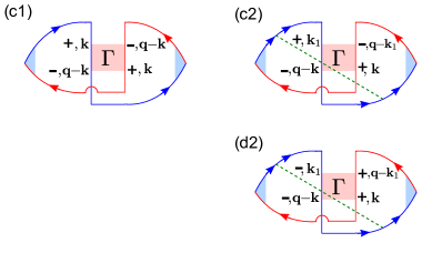
Figure 8: The Feynman diagrams for the quantum interference correction to the conductivity that take into account the Cooperons from the intervalley scattering Lu et al. (2013). These diagrams give $\sigma^{qi}_{I}$.

The conductivity contribution from the intervalley Cooperons is given by (see Fig. 8)

$$\sigma^{qi}_{I}=2\times(\sigma_{c1}+2\times\sigma_{c2}+2\times\sigma_{d2}),$$ (43)

where

$$\sigma_{c1} = \frac{e^{2}\hbar}{2\pi}\sum_{\mathbf{q}}\Gamma^{+-}_{-+}(\mathbf{k},-\mathbf{k})$$

$$\times\sum_{\mathbf{k}}\widetilde{v}^{x}_{\mathbf{k},+}G^{R}_{\mathbf{k},+}G^{R}_{\mathbf{q}-\mathbf{k},-}\widetilde{v}^{x}_{\mathbf{q}-\mathbf{k},-}G^{A}_{\mathbf{q}-\mathbf{k},-}G^{A}_{\mathbf{k},+},$$

$$\sigma_{c2} = \frac{e^{2}\hbar}{2\pi}\sum_{\mathbf{q}}\Gamma^{+-}_{-+}(\mathbf{k}_{1},-\mathbf{k})$$

$$\times\sum_{\mathbf{k}}\sum_{\mathbf{k}_{1}}\widetilde{v}^{x}_{\mathbf{k},+}G^{R}_{\mathbf{k},+}G^{R}_{\mathbf{k}_{1},+}G^{R}_{\mathbf{q-k},-}G^{R}_{\mathbf{q-k_{1}},-}$$

$$\times\widetilde{v}^{x}_{\mathbf{q}-\mathbf{k}_{1},-}G^{A}_{\mathbf{q}-\mathbf{k}_{1},-}G^{A}_{\mathbf{k},+}\langle U^{++}_{\mathbf{k},\mathbf{k}_{1}}U^{--}_{\mathbf{q-k},\mathbf{q-k_{1}}}\rangle,$$

$$\sigma_{d2} = \frac{e^{2}\hbar}{2\pi}\sum_{\mathbf{q}}\Gamma^{--}_{++}(\mathbf{k}_{1},-\mathbf{k})$$ (44)

$$\times\sum_{\mathbf{k}}\sum_{\mathbf{k}_{1}}\widetilde{v}^{x}_{\mathbf{k},t}G^{R}_{\mathbf{k},+}G^{R}_{\mathbf{k}_{1},-}G^{R}_{\mathbf{q}-\mathbf{k},-}G^{R}_{\mathbf{q}-\mathbf{k}_{1},+}$$

$$\times\widetilde{v}^{x}_{\mathbf{q}-\mathbf{k}_{1},+}G^{A}_{\mathbf{q}-\mathbf{k}_{1},+}G^{A}_{\mathbf{k},+}\langle U^{+-}_{\mathbf{k},\mathbf{k}_{1}}U^{-+}_{\mathbf{q}-\mathbf{k},\mathbf{q}-\mathbf{k}_{1}}\rangle.$$

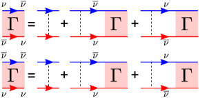
Figure 9: The Feynman diagrams of the Bethe-Salpeter equations for the intervalley Cooperons. $\nu$ is the valley index, $\nu=\pm$, $\overline{\nu}=-$ if $\nu=+$.

In polar coordinates, the intervalley Cooperons can be found from the coupled Bethe-Salpeter equations (see Fig. 9)

$$\Gamma^{+-}_{-+}(\mathbf{k}_{1},\mathbf{k}_{2})$$

$$= \gamma^{+-}_{-+}(\mathbf{k}_{1},\mathbf{k}_{2})+\int_{0}^{2\pi}\frac{d\varphi}{2\pi}\int_{0}^{\pi}\frac{d\theta\sin\theta}{2\pi}$$

$$\times\int_{0}^{\infty}\frac{dkk^{2}}{2\pi}\sum_{\nu=\pm}\gamma^{+\nu}_{-\overline{\nu}}(\mathbf{k}_{1},\mathbf{k})\mathcal{G}_{\mathbf{k}}^{i\epsilon_{n}}\mathcal{G}_{\mathbf{q-k}}^{i\epsilon_{n}-i\omega_{m}}\Gamma^{\nu-}_{\overline{\nu}+}(\mathbf{k},\mathbf{k}_{2}),$$

$$\Gamma^{--}_{++}(\mathbf{k}_{1},\mathbf{k}_{2})$$

$$= \gamma^{--}_{++}(\mathbf{k}_{1},\mathbf{k}_{2})+\int_{0}^{2\pi}\frac{d\varphi}{2\pi}\int_{0}^{\pi}\frac{d\theta\sin\theta}{2\pi}$$

$$\times\int_{0}^{\infty}\frac{dkk^{2}}{2\pi}\sum_{\nu=\pm}\gamma^{-\nu}_{+\overline{\nu}}(\mathbf{k}_{1},\mathbf{k})\mathcal{G}_{\mathbf{k}}^{i\epsilon_{n}}\mathcal{G}_{\mathbf{q-k}}^{i\epsilon_{n}-i\omega_{m}}\Gamma^{\nu-}_{\overline{\nu}+}(\mathbf{k},\mathbf{k}_{2}),$$

where $\overline{\nu}=-$ if $\nu=+$ and

$$\gamma^{\nu\overline{\nu}}_{\overline{\nu}\nu}(\mathbf{k}_{1},\mathbf{k}_{2})\equiv\langle U^{\nu\overline{\nu}}_{\mathbf{k}_{1},\mathbf{k}_{2}}U^{\overline{\nu}\nu}_{-\mathbf{k}_{1},-\mathbf{k}_{2}}\rangle$$ (46)

$$= \frac{\hbar\eta_{I}}{2\pi N_{F}\tau}[\frac{1}{2}(1+\nu\cos\theta_{1})(1+\overline{\nu}\cos\theta_{2})$$

$$-\sin\theta_{1}\sin\theta_{2}e^{i(\varphi_{2}-\varphi_{1})}$$

$$+\frac{1}{2}(1+\overline{\nu}\cos\theta_{1})(1+\nu\cos\theta_{2})e^{i2(\varphi_{2}-\varphi_{1})}],$$

$$\gamma^{\nu\nu}_{\overline{\nu}\overline{\nu}}(\mathbf{k}_{1},\mathbf{k}_{2})\equiv\langle U^{\nu\nu}_{\mathbf{k}_{1},\mathbf{k}_{2}}U^{\overline{\nu}\overline{\nu}}_{-\mathbf{k}_{1},-\mathbf{k}_{2}}\rangle$$

$$= \frac{\hbar\eta_{*}}{2\pi N_{F}\tau}[\frac{1}{2}(1+\nu\cos\theta_{1})(1+\nu\cos\theta_{2})$$

$$+\sin\theta_{1}\sin\theta_{2}e^{i(\varphi_{2}-\varphi_{1})}$$

$$+\frac{1}{2}(1+\overline{\nu}\cos\theta_{1})(1+\overline{\nu}\cos\theta_{2})e^{i2(\varphi_{2}-\varphi_{1})}],$$

where $\nu=\pm$, $\eta_{I}\equiv\tau/\tau_{I}$, and $\eta_{*}\equiv\tau/\tau_{*}$. We assume

$$\Gamma^{+-}_{-+}(\mathbf{k}_{1},\mathbf{k}_{2}) = \frac{\hbar}{2\pi N_{F}\tau}[a_{1}(1+\cos\theta_{1})(1-\cos\theta_{2})$$

$$-a_{2}\sin\theta_{1}\sin\theta_{2}e^{i(\varphi_{2}-\varphi_{1})}$$

$$+a_{3}(1-\cos\theta_{1})(1+\cos\theta_{2})e^{i2(\varphi_{2}-\varphi_{1})}],$$

$$\Gamma^{--}_{++}(\mathbf{k}_{1},\mathbf{k}_{2}) = \frac{\hbar}{2\pi N_{F}\tau}[b_{1}(1-\cos\theta_{1})(1-\cos\theta_{2})$$

$$+b_{2}\sin\theta_{1}\sin\theta_{2}e^{i(\varphi_{2}-\varphi_{1})}$$

$$+b_{3}(1+\cos\theta_{1})(1+\cos\theta_{2})e^{i2(\varphi_{2}-\varphi_{1})}],$$

and put them into the Bethe-Salpeter equations, we arrive at

$$a_{1}=a_{3} = \frac{1}{2\ell^{2}}\frac{\chi_{1}^{a}}{Q_{1}^{2}+q^{2}},\ \ a_{2}=\frac{1}{\ell^{2}}\frac{\chi_{2}^{a}}{Q_{2}^{2}+q^{2}},$$

$$b_{1}=b_{3} = \frac{1}{2\ell^{2}}\frac{\chi_{1}^{b}}{Q_{1}^{2}+q^{2}},\ \ b_{2}=\frac{1}{\ell^{2}}\frac{\chi_{2}^{b}}{Q_{2}^{2}+q^{2}},$$ (48)

where $q^{2}=q_{x}^{2}+q_{y}^{2}+q_{z}^{2}$ and other quantities are defined in Eq. (VIII.3).

VIII.3 Conductivity and magnetoconductivity from quantum interference

The total conductivity from the quantum interference has two parts

$$\sigma^{qi} = 2\times\sigma^{qi}_{0}+\sigma^{qi}_{I}.$$ (49)

For a single valley,

$$\sigma^{qi}_{0} \approx \frac{e^{2}}{h}\frac{2+\eta_{I}}{(1+\eta_{I})^{2}}\sum_{\mathbf{q}}\frac{1}{Q_{0}^{2}+q^{2}},$$ (50)

where

$$Q_{0}^{2}\equiv\frac{(2+\eta_{I})\eta_{I}}{2(1-\eta_{I})}\frac{1}{\ell^{2}}$$ (51)

and $\eta_{I}=\tau/\tau_{I}$ measures the weight of the intervalley scattering in the total scattering. The total scattering time $\tau$ is defined as $1/\tau=1/\tau_{0}+1/\tau_{I}$, $\tau_{0}$ and $\tau_{I}$ are the intravalley and intervalley scattering times, respectively.

The intervalley part

$$\sigma^{qi}_{I}=2\times(\sigma_{c1}+2\times\sigma_{c2}+2\times\sigma_{d2}),$$ (52)

where

$$\sigma_{c1}^{x} = -\frac{e^{2}}{h}\frac{1}{(1+\eta_{I})^{2}}\sum_{\mathbf{q}}(\frac{18}{5}\frac{\chi_{1}^{a}}{Q_{1}^{2}+q^{2}}+\frac{12}{5}\frac{\chi_{2}^{a}}{Q_{2}^{2}+q^{2}}),$$

$$\sigma_{c2}^{x} = \frac{e^{2}}{h}\frac{1}{(1+\eta_{I})^{2}}\sum_{\mathbf{q}}\frac{\eta_{*}}{2}(\frac{\chi_{1}^{a}}{Q_{1}^{2}+q^{2}}+\frac{\chi_{2}^{a}}{Q_{2}^{2}+q^{2}}),$$

$$\sigma_{d2}^{x} = -\frac{e^{2}}{h}\frac{1}{(1+\eta_{I})^{2}}\sum_{\mathbf{q}}\frac{\eta_{I}}{2}(\frac{\chi_{1}^{b}}{Q_{1}^{2}+q^{2}}+\frac{\chi_{2}^{b}}{Q_{2}^{2}+q^{2}}),$$ (53)

and $q^{2}=q_{x}^{2}+q_{y}^{2}+q_{z}^{2}$,

$$Q_{1}^{2} = \frac{(1-\frac{2}{3}\eta_{*})^{2}-(\frac{2}{3}\eta_{I})^{2}}{\varpi_{1}\ell^{2}},\ Q_{2}^{2}=\frac{(1-\frac{2}{3}\eta_{*})^{2}-(\frac{2}{3}\eta_{I})^{2}}{\varpi_{2}\ell^{2}},$$

$$\chi_{1}^{a} = \eta_{I}/\varpi_{1},\ \ \chi_{1}^{b}=[\eta_{*}+2(\eta_{I}^{2}-\eta_{*}^{2})/3]/\varpi_{2},$$

$$\chi_{2}^{a} = \eta_{I}/\varpi_{2},\ \ \chi_{2}^{b}=[\eta_{*}+2(\eta_{I}^{2}-\eta_{*}^{2})/3]/\varpi_{2},$$

$$\varpi_{1} = \frac{16}{15}\eta_{*}+\frac{22}{45}(\eta_{I}^{2}-\eta_{*}^{2}),\ \varpi_{2}=\frac{8}{15}\eta_{*}+\frac{16}{45}(\eta_{I}^{2}-\eta_{*}^{2}),$$

$$\eta_{I} = \tau/\tau_{I},\ \ \eta_{*}=\tau/\tau_{*}.$$ (54)

One can check that $\sigma^{qi}_{I}$ vanishes when $\eta_{I}=0$.

To have the temperature dependence of the conductivity, one just replaces all the $\sum_{\mathbf{q}}\frac{1}{Q_{i}^{2}+q^{2}}$ in $\sigma^{qi}$ by

$$\frac{1}{2\pi^{2}}\int_{1/\ell_{\phi}}^{1/\ell}q^{2}dq.$$ (55)

The temperature dependence is contained in the phase coherence length $\ell_{\phi}=C/T^{p/2}$, $C$ is a constant. In three dimensions, $p=3/2$ ($p=3$) if the electron-electron (electron-phonon) interaction is the decoherence mechanism Lee and Ramakrishnan (1985).

To calculate the magnetoconductivity, one just replaces all the $\sum_{\mathbf{q}}\frac{1}{Q_{i}^{2}+q^{2}}$ in $\sigma^{qi}$ by

$$\Psi_{3}(B,Q_{i}) = \int_{0}^{1/\ell}\frac{dx}{(2\pi)^{2}}\left[\psi\left(\frac{\ell_{B}^{2}}{\ell^{2}}+\ell_{B}^{2}(Q_{i}^{2}+x^{2})+\frac{1}{2}\right)\right.$$ (56)

$$\left.-\psi\left(\frac{\ell_{B}^{2}}{\ell_{\phi}^{2}}+\ell_{B}^{2}(Q_{i}^{2}+x^{2})+\frac{1}{2}\right)\right],$$

where the magnetic length $\ell_{B}\equiv\sqrt{\hbar/4eB}$, the magnetic field $B$ is along arbitrary directions. The magnetoconductivity is defined as

$$\delta\sigma^{qi}(B)\equiv\sigma^{qi}(B)-\sigma^{qi}(0).$$ (57)

VIII.4 Conductivity and magnetoconductivity of a single valley of Weyl fermions

For a single valley in absence of intervalley scattering, $\sigma^{qi}$ reduces to $\sigma^{qi}_{0}$ in Eq. (50) with $\eta_{I}=0$,

$$\sigma^{qi}=\frac{e^{2}}{h}2\sum_{\mathbf{q}}\frac{1}{q^{2}}.$$ (58)

Replace the summation by the integral in Eq. (55),

$$\sigma^{qi}=\frac{e^{2}}{h}2\frac{1}{2\pi^{2}}\int_{1/\ell_{\phi}}^{1/\ell}dq\frac{1}{q^{2}}q^{2}=\frac{e^{2}}{h}\frac{1}{\pi^{2}}(\frac{1}{\ell}-\frac{1}{\ell_{\phi}}).$$ (59)

This is of the same magnitude of Eq. (2.25a) of Ref. Lee and Ramakrishnan, 1985 but differs by a minus sign (note that spin degeneracy 2 is included in Ref. Lee and Ramakrishnan, 1985).

Replace the summation in Eq. (58) by Eq. (56), $\sigma^{qi}(B)$ of a single valley is found as

$$\sigma^{qi}(B)=\frac{e^{2}}{h}2\Psi_{3}(B),$$ (60)

and the magnetoconductivity is

$$\delta\sigma^{qi}(B) \equiv \sigma^{qi}(B)-\sigma^{qi}(0),$$

where

$$\sigma^{qi}(B) = \frac{2e^{2}}{h}\int_{0}^{1/\ell}\frac{dx}{(2\pi)^{2}}\left[\psi\left(\frac{\ell_{B}^{2}}{\ell^{2}}+\ell_{B}^{2}x^{2}+\frac{1}{2}\right)\right.$$ (62)

$$\left.-\psi\left(\frac{\ell_{B}^{2}}{\ell_{\phi}^{2}}+\ell_{B}^{2}x^{2}+\frac{1}{2}\right)\right],$$

where the magnetic length $\ell_{B}\equiv\sqrt{\hbar/4eB}$, the magnetic field $B$ is along arbitrary directions, $\ell$ is the mean free path, and $\ell_{\phi}$ is the phase coherence length.

IX Conductivity correction from interaction

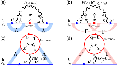
Figure 10: The Feynman diagrams for the self-energies arising from the interplay of electron-electron interaction and disorder scattering Altshuler et al. (1980); Fukuyama (1980).

The leading-order of the self-energy from the interplay of interaction and disorder is the Fock (exchange) diagram dressed by Diffusons [see Fig. 10(a)],

$$\Sigma^{F}_{D}(\mathbf{k},i\epsilon_{n}) = -\frac{1}{\beta}\sum_{\omega_{m}}\sum_{\mathbf{q}}\mathcal{G}_{\mathbf{k}-\mathbf{q}}^{i\epsilon_{n}-i\omega_{m}}\sum_{\mathbf{k}^{\prime}}\sum_{\mathbf{k}^{\prime\prime}}V(\mathbf{q},i\omega_{m})$$ (63)

$$\times\Lambda^{\mathbf{k}\rightarrow\mathbf{k}^{\prime},i\epsilon_{n}}_{\mathbf{k}-\mathbf{q}\leftarrow\mathbf{k}^{\prime}-\mathbf{q},i\epsilon_{n}-i\omega_{m}}\Lambda^{\mathbf{k}^{\prime\prime}\rightarrow\mathbf{k},i\epsilon_{n}}_{\mathbf{k}^{\prime\prime}-\mathbf{q}\leftarrow\mathbf{k}-\mathbf{q},i\epsilon_{n}-i\omega_{m}}$$

$$\times\mathcal{G}_{\mathbf{k}^{\prime}}^{i\epsilon_{n}}\mathcal{G}_{\mathbf{k}^{\prime}-\mathbf{q}}^{i\epsilon_{n}-i\omega_{m}}\mathcal{G}_{\mathbf{k}^{\prime\prime}-\mathbf{q}}^{i\epsilon_{n}-i\omega_{m}}\mathcal{G}_{\mathbf{k}^{\prime\prime}}^{i\epsilon_{n}},$$

where $1/\beta=k_{B}T$, later we will show how to calculate the Diffuson $\Lambda$ and interaction $V$. We find that (Sec. IX.1)

$$\Lambda^{\mathbf{k}\rightarrow\mathbf{k}^{\prime},i\epsilon_{n}}_{\mathbf{k}-\mathbf{q}\leftarrow\mathbf{k}^{\prime}-\mathbf{q},i\epsilon_{n}-i\omega_{m}}=\Lambda^{\mathbf{k}^{\prime\prime}\rightarrow\mathbf{k},i\epsilon_{n}}_{\mathbf{k}^{\prime\prime}-\mathbf{q}\leftarrow\mathbf{k}-\mathbf{q},i\epsilon_{n}-i\omega_{m}}$$ (64)

$$= \Lambda_{\mathbf{k}_{1},\mathbf{k}_{2}}\approx\frac{\hbar}{2\pi N_{F}\tau^{2}}\frac{1}{\omega_{m}+Dq^{2}},$$

and

$$\sum_{\mathbf{k}^{\prime}}\mathcal{G}_{\mathbf{k}^{\prime}}^{i\epsilon_{n}}\mathcal{G}_{\mathbf{k}^{\prime}-\mathbf{q}}^{i\epsilon_{n}-i\omega_{m}}\approx\frac{2\pi N_{F}\tau}{\hbar}\theta[\epsilon_{n}(\omega_{m}-\epsilon_{n})].$$ (65)

Then

$$\Sigma^{F}_{D}(\mathbf{k},i\epsilon_{n})$$

$$\approx -\frac{1}{\beta}\sum_{\omega_{m}}\mathcal{G}_{\mathbf{k}}^{i\epsilon_{n}-i\omega_{m}}\frac{1}{\tau^{2}}\sum_{\mathbf{q}}\frac{V_{\mathbf{q}}^{i\omega_{m}}\theta[\epsilon_{n}(\omega_{m}-\epsilon_{n})]}{(\omega_{m}+Dq^{2})^{2}}.$$

It is of the same form as Eq. (3.16) in Ref. Altshuler and Aronov, 1985. Therefore, the leading-order self-energy and its associated contribution to the conductivity has the same form as that for the conventional electron with dispersion $p^{2}/2m$. The difference is that $D$ and $N_{F}$ need to be changed to those for the Weyl fermions.

IX.1 Diffuson

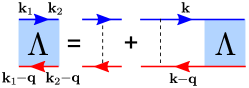
Figure 11: The Feynman diagrams of the Bethe-Salpeter equations for the Diffuson.

In polar coordinates, the Diffuson can be found from the Bethe-Salpeter equation (see Fig. 11)

$$\Lambda_{\mathbf{k}_{1},\mathbf{k}_{2}} = \Lambda_{\mathbf{k}_{1},\mathbf{k}_{2}}^{0}+\int_{0}^{2\pi}\frac{d\varphi}{2\pi}\int_{0}^{\pi}\frac{d\theta\sin\theta}{2\pi}\int_{0}^{\infty}\frac{dkk^{2}}{2\pi}$$ (67)

$$\times\Lambda_{\mathbf{k}_{1},\mathbf{k}}^{0}\mathcal{G}_{\mathbf{k}}^{i\epsilon_{n}}\mathcal{G}_{\mathbf{k-q}}^{i\epsilon_{n}-i\omega_{m}}\Lambda_{\mathbf{k},\mathbf{k}_{2}},$$

where the bare Diffuson can be found

$$\Lambda^{0}_{\mathbf{k}_{1},\mathbf{k}_{2}}\equiv\langle U_{\mathbf{k}_{1},\mathbf{k}_{2}}U_{\mathbf{k}_{2},\mathbf{k}_{1}}\rangle$$ (68)

$$\approx \frac{\hbar}{2\pi N_{F}\tau}[1+(1-2\eta_{I})$$

$$\times(\cos\theta_{1}\cos\theta_{2}+\sin\theta_{1}\sin\theta_{2}\cos(\varphi_{1}-\varphi_{2}))],$$

and it can be found that

$$\int_{0}^{\infty}\frac{dkk^{2}}{2\pi}\mathcal{G}_{\mathbf{k}}^{i\epsilon_{n}}\mathcal{G}_{\mathbf{k-q}}^{i\epsilon_{n}-i\omega_{m}}=\frac{2\pi^{2}N_{F}\tau}{\hbar}\frac{1}{1+\omega_{m}\tau+i\tau\mathbf{v}_{F}\cdot\mathbf{q}}.$$

For convenience, the $z$-axis of $\mathbf{k}$ can be chosen to be along the direction of $\mathbf{q}$, then $\mathbf{v}_{F}\cdot\mathbf{q}=v_{F}q\cos\theta$ and

$$\frac{1}{1+\omega_{m}\tau+i\tau\mathbf{v}_{F}\cdot\mathbf{q}}$$ (70)

$$\approx 1-\omega_{m}\tau-i\tau v_{F}q\cos\theta-\tau^{2}v_{F}^{2}q^{2}\cos^{2}\theta.$$

We assume the form of the full Diffuson to be

$$\Lambda_{\mathbf{k}_{1},\mathbf{k}_{2}} \approx \frac{\hbar}{2\pi N_{F}\tau}[d_{1}+d_{2}\cos\theta_{1}+d_{3}\cos\theta_{2}$$

$$+d_{4}\cos\theta_{1}\cos\theta_{2}+d_{5}\sin\theta_{1}\sin\theta_{2}\cos(\varphi_{1}-\varphi_{2})],$$

with the coefficients $d_{i}$ to be determined. By putting it into the Bethe-Salpeter equation, we find that only the $d_{1}$ term is divergent as $q,\omega_{m}\rightarrow 0$ and

$$\Lambda_{\mathbf{k}_{1},\mathbf{k}_{2}} \approx \frac{\hbar}{2\pi N_{F}\tau^{2}}\frac{1}{\omega_{m}+Dq^{2}},$$ (72)

where the diffusion coefficient

$$D=\frac{1}{3}v_{F}^{2}\tau\eta_{v}.$$ (73)

It is worth noting that here the expression of $D$ derived from the Diffuson coincides with that in the semiclassical conductivity (Sec. VII). The above calculation does not distinguish inter- and intra-valley scattering $\Lambda=\Lambda^{++}_{++}+\Lambda^{+-}_{+-}$.

IX.2 Interaction and random phase approximation

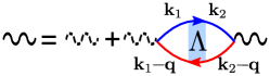
Figure 12: The Feynman diagram for the interaction (dashed wavy lines for bare interaction), which is renormalized (solid wavy lines) under random phase approximation. Different from in a clean system, the density function is dressed by the Diffuson ($\Lambda$).

Figure 13: (a) The screening factor $F$ as a function of $x=8\pi^{2}v_{F}\hbar\varepsilon/e^{2}$ for Weyl fermions. $v_{F}$ is the Fermi velocity. $\hbar$ is the reduced Planck’s constant. $\varepsilon$ is the dielectric constant. $-e$ is the electron charge. (b) In three dimensions, $\widetilde{F}$ as a function of $F$. $\tilde{F}$ is the renormalized screening factor after including the second-order diagrams and correction of the disorder by the interaction.

After the Fourier transformation, the Hamiltonian of the interaction becomes

$$V=\sum_{\mathbf{k},\mathbf{k}^{\prime},\mathbf{q}}\frac{V_{\mathbf{q}}}{2}(\phi_{\mathbf{k}}^{\dagger}\cdot\phi_{\mathbf{k}+\mathbf{q}})(\phi_{\mathbf{k}^{\prime}}^{\dagger}\cdot\phi_{\mathbf{k}^{\prime}-\mathbf{q}})c^{{\dagger}}_{\mathbf{k}^{\prime}}c^{{\dagger}}_{\mathbf{k}}c_{\mathbf{k}+\mathbf{q}}c_{\mathbf{k}^{\prime}-\mathbf{q}},$$

where $\phi$’s are the spinor wave functions, $c$’s are corresponding operators, and

$$V_{\mathbf{q}}=\int\mathrm{d}^{3}\mathbf{r}\frac{e^{2}}{4\pi\varepsilon r}e^{-\mathrm{i}\mathbf{q}\cdot\mathbf{r}}=\frac{e^{2}}{\varepsilon q^{2}}$$ (75)

with $\varepsilon$ the dielectric constant. Because $v_{q}$ diverges as $q\rightarrow 0$, then the spinor wave function part vanishes for a single band in the interaction potential

$$V_{0}(q)=v_{\mathbf{q}}(\phi_{\mathbf{k}}^{\dagger}\cdot\phi_{\mathbf{k}+\mathbf{q}})(\phi_{\mathbf{k}^{\prime}}^{\dagger}\cdot\phi_{\mathbf{k}^{\prime}-\mathbf{q}})\approx V_{\mathbf{q}}.$$ (76)

The long-range (bare) interaction is renormalized under the random phase approximation (see Fig. 12)

$$V(\mathbf{q},\omega_{m}) = \frac{V_{0}(q)}{1+V_{0}(q)\Pi(q,\omega_{m})},$$ (77)

where different from in a clean system, the density response function in a disordered system is dressed by the Diffuson and takes the form

$$\Pi(\mathbf{q},\omega_{m}) = N_{F}\frac{Dq^{2}}{\omega_{m}+Dq^{2}}.$$ (78)

Then

$$V(\mathbf{q},i\omega_{m}) = \frac{e^{2}}{\varepsilon q^{2}+e^{2}N_{F}\frac{Dq^{2}}{\omega_{m}+Dq^{2}}}.$$ (79)

In the limit that $\omega_{m},\ q\rightarrow 0$, the dynamically-screened interaction becomes

$$V(\mathbf{q},i\omega_{m})\approx\frac{1}{N_{F}}\frac{\omega_{m}+Dq^{2}}{Dq^{2}}.$$ (80)

This renormalized interaction is the one that is used in calculating the self-energy induced by the interplay of interaction and disorder.

IX.3 Screening factor

The contribution from other three one-loop interaction diagrams [see Fig. 10 (b)-(d)] is proportional to the screening factor $F$, which is defined as

$$F\equiv\frac{\langle V(\mathbf{k}-\mathbf{k}^{\prime})\rangle_{k_{F}}}{V(0)},$$ (81)

where $\langle...\rangle_{k_{F}}$ means the average of the interaction $V(\mathbf{k}-\mathbf{k}^{\prime})$ over momenta $\mathbf{k}$ and $\mathbf{k}^{\prime}$ on the Fermi surface.

In three dimensions Altshuler and Aronov (1985),

$$F = \frac{\ln[(1+(2k_{F}\xi)^{2}]}{(2k_{F}\xi)^{2}},$$ (82)

where $k_{F}$ the Fermi wave vector and $\xi$ is the screening length of the interaction,

$$\xi^{2}=\frac{\varepsilon}{e^{2}N_{F}}.$$ (83)

Using the density of states for the Weyl fermions $N_{F}=E_{F}^{2}/2\pi^{2}(v_{F}\hbar)^{3}$ and $E_{F}=v_{F}\hbar k_{F}$, we define

$$x\equiv(2k_{F}\xi)^{2}=\frac{8\pi^{2}v_{F}\hbar\varepsilon}{e^{2}}.$$ (84)

Fig. 13 shows $F$ as a function of $x$. By definition, $F\in[0,1]$.

The screening factor $F$ will be renormalized after including the second-order diagrams and correction of the disorder by the interaction. The renormalized screening factor in three dimensions is Altshuler and Aronov (1985)

$$\widetilde{F}=-\frac{32}{3}[1+\frac{3F}{4}-(1+\frac{F}{2})^{3/2}]F,$$ (85)

which is shown in Fig. 13 as a function of $F$. One can see that $\widetilde{F}\approx F$ as $F\rightarrow 0$ and $\widetilde{F}\approx 0.93F$ as $F\rightarrow 1$.

X Classical magnetoconductivity from Lorentz force

The classical negative magnetoconductivity as a result of the cyclotron motion driven by Lorentz force in a perpendicular magnetic field $B$ can be found as Datta (1997)

$$\delta\sigma^{C}(B) = -\sigma^{sc}(\mu B)^{2},$$ (86)

where $\sigma^{sc}$ is given by Eq. (30) and $\mu$ is given by Eq. (88). We arrive at

$$\delta\sigma^{C}(B) = -\frac{e^{2}}{h}\frac{\ell^{3}\sqrt{3}\eta_{v}^{3/2}}{16\pi\ell_{B}^{4}}$$ (87)

$$= -\frac{e^{2}}{h}\frac{9}{32\sqrt{2}\pi(1+\eta_{I})^{3/2}}\frac{\ell^{3}}{\ell_{B}^{4}},$$

where $\ell_{B}\equiv\sqrt{\hbar/4eB}$.

The mobility of one valley of Weyl fermion is found as

$$\mu = \frac{ev_{F}\tau\eta_{v}}{\hbar k_{F}}=\frac{e\ell\sqrt{3\eta_{v}}}{\hbar k_{F}}\approx\frac{e\ell}{\hbar k_{F}},$$ (88)

where the mean free path $\ell\equiv\sqrt{D\tau}=v_{F}\tau\sqrt{\eta_{v}/3}\approx v_{F}\tau$.

The relation between the mobility and mean free path is approximated as

$$\ell\approx\frac{\mu\hbar k_{F}}{e}\approx 66\mu k_{F},$$ (89)

where $\ell$ in nm, $\mu$ is in cm²/(V$\cdot$s), and $k_{F}$ in $\AA^{-1}$. For $k_{F}=0.03$ and $\mu=10^{4}$, the mean free path is about $20\mu$m.

XI conclusions

In this work, we study the quantum transport properties of a two-valley Weyl semimetal. We employ the Feynman diagram techniques to calculate the conductivity in the presence of disorder and interaction. We derive three dominant parts of the conductivity (see Fig. 1), including the semiclassical (Drude) conductivity, the correction from the quantum interference [weak (anti-)localization] , and the correction from the interplay of electron-electron interaction and disorder scattering (Altshuler-Aronov effect).

The quantum interference gives the main contribution to the magnetoconductivity. For a single valley of Weyl fermions, the low-temperature magnetoconductivity is proportional to $-\sqrt{B}$, where $B$ is the magnetic field applied along arbitrary directions [see Fig. 3 (a)]. This $-\sqrt{B}$ magnetoconductivity is from the weak antilocalization of Weyl fermions in the presence of weak inter-valley scattering. Near zero field, the $-\sqrt{B}$ magnetoconductivity always overwhelms the positive $B^{2}$ magnetoconductivity from the chiral anomaly, giving another transport signature of Weyl semimetals. Strong inter-valley scattering and correlation can lead to a crossover from the weak antilocalization to weak localization. During the crossover, the $-\sqrt{B}$ magnetoconductivity turns to $\sqrt{B}$ in the limit of strong inter-valley scattering and correlation [see Fig. 3 (c)]. By including the contributions from the weak antilocalization, Berry curvature correction, and Lorentz force (Tab. 2), we compare the calculated magnetoconductivity with a recent experiment (see Fig. 4).

Both the quantum interference and interaction contribute to the temperature dependence of the conductivity. For a single valley of Weyl fermions, the weak antilocalization from the quantum interference gives a conductivity proportional to $-T^{p/2}$ , where $T$ is the temperature and the parameter $p$ is positive and depends on decoherence mechanisms. This conductivity thus always increases with decreasing temperature, giving another signature of the weak antilocalization. In contrast, the interaction gives a conductivity that decreases with decreasing temperature, following a $\sqrt{T}$ dependence. Therefore, we expect a competition in the temperature dependence of the conductivity (see Fig. 2). Because $p$ is usually greater than $1$, the interaction always dominates below a critical temperature, leading to a tendency to localization in the temperature-dependent conductivity.

We also present a systematic comparison of the transport properties for a single valley of Weyl fermions, 2D massless Dirac fermions, and 3D conventional electrons (Table 3).